Enhanced Rolling Bearing Fault Diagnosis Using Multimodal Deep Learning and Singular Spectrum Analysis

Abstract

A decision-level multimodal fusion deep learning strategy is proposed for the effective fault detection of rolling bearings based on long-term fault signals collected from multiple sensors. First, key features are extracted from the multimodal signal set using singular spectrum analysis (SSA), and these features are transformed into a composite dataset that combines short-time Fourier transform (STFT) images and time series data. Based on this, a recursive gated convolutional neural network (RGCNN) is designed to process the STFT image data, while a 1D convolutional neural network (1DCNN) is specifically optimized for training with time series data. Furthermore, decision-level multimodal feature fusion is achieved by applying a weighted average method to integrate the features from different deep learning models, aiming to obtain more comprehensive fault prediction results. The proposed method, multimodal fusion fault detection (MFFD), is validated on the Paderborn and Ottawa rolling bearing datasets, which include various typical faults. Experimental results demonstrate the effectiveness of the proposed approach. Compared to traditional single-modality deep learning models, the proposed method shows significant improvements in fault diagnosis accuracy and generalization capability.

1. Introduction

The health monitoring and fault diagnosis of rolling bearings are critical for ensuring the normal operation of mechanical equipment [1]. The stable and safe operation of rolling bearings directly impacts the overall stability and efficiency of the entire system. Traditional fault diagnosis methods based on single-modal signals have certain limitations as they cannot comprehensively and accurately reflect the operating conditions and health status of bearing gearboxes, thus restricting their performance in terms of accuracy and efficiency [2]. Considering the high-pressure and high-temperature characteristics of the bearing’s working environment, the importance of these monitoring and diagnosis processes is further heightened.

On the one hand, physics-based methods perform fault diagnosis by simulating the dynamic behavior of the equipment [3,4,5]. While these methods have a practical physical background, their accuracy in establishment and application may be challenged as the complexity of the equipment increases. On the other hand, data-driven models construct predictive models by analyzing and processing equipment data [6,7,8]. Despite facing challenges regarding data quality and quantity, they exhibit excellent predictive accuracy and have become the current mainstream technology.

Multimodal refers specifically to the features of different sensors or signal sources, which may differ in physical properties or measurement modalities. Existing multimodal signal fusion methods attempt to integrate features from different signals [9,10]; however, due to a lack of effective modal representation mechanisms, the fusion of features between different signals may not be ideal, limiting the full utilization of key information in multimodal signals. Therefore, the health monitoring and fault diagnosis of rolling bearings need to overcome the limitations of single-modal and multimodal signal fusion to achieve a more comprehensive and accurate assessment of bearing health status and fault prediction.

In recent years, with significant advancements in computer hardware and the rapid iteration of algorithmic models, the application of deep learning techniques in the field of rotating machinery fault detection has been rapidly increasing [11,12,13,14]. These models extract deep features from raw data by cascading multiple layers of nonlinear modules within the deep learning framework. Since deep learning models are typically end-to-end, they can obtain features without manual intervention, enhancing their application scenarios. Currently, various deep learning models, such as multilayer perceptron (MLP) [15], convolutional neural networks (CNNs) [16,17], one-dimensional convolutional neural networks, and graph convolutional networks (GCNs) [18], have been widely used in the fault diagnosis of rotating machinery, and the results obtained have been significant. However, CNNs also have drawbacks, especially due to vanishing or exploding gradients, which make it difficult to achieve fault classification with a high number of convolutional layers. Therefore, a one-dimensional convolutional neural network (1DCNN) was proposed to simplify the structure of the CNN and maximize the classification accuracy [19,20,21]. In addition, the recursive gated ${\mathrm{g}}^{\mathrm{n}}\mathrm{C}\mathrm{o}\mathrm{n}\mathrm{v}$ method proposed in the literature [22] provides an effective solution through a higher-order attention mechanism and the learning of distant features. ${\mathrm{g}}^{\mathrm{n}}\mathrm{C}\mathrm{o}\mathrm{n}\mathrm{v}$ (n denotes the order of the higher-order interactions) combines the gated convolution and the recursive design, which is able to realize the higher-order spatial interactions and thus extract effective higher-order features. Therefore, in this study, we combine the 1DCNN, MLP, and ${\mathrm{g}}^{\mathrm{n}}\mathrm{C}\mathrm{o}\mathrm{n}\mathrm{v}$ methods for better fault classification and feature extraction to improve the accuracy and robustness of the model.

However, most existing studies rely on fault features derived from a single modality [23,24]. Such data are vulnerable to external factors, such as sensor malfunctions and strong noise interference, which can negatively affect the accuracy of diagnostic models. To address this limitation, a signal decomposition method called singular spectral decomposition (SSD) is proposed with the help of singular spectral analysis (SSA) [25], and it has excellent resistance to noise interference. Therefore, it is meaningful and necessary to use this method to separate the strong interference background from weak fault signals for the fault diagnosis of rolling bearings.

Moreover, rotating machinery is a complex system composed of multiple components, typically monitored by multiple sensors simultaneously. Therefore, utilizing multimodal sensor data to build and train models is of great importance for improving the accuracy of equipment fault diagnosis [26].

This paper focuses on the bearing gearbox as the research object and introduces a multi-modal fusion model and decision fusion strategy. By combining various signal modalities, such as vibration, acoustic, and electrical signals, we conduct a comprehensive analysis aimed at investigating fault diagnosis techniques based on multi-modal signals. We have established effective fusion strategies for multiple modalities, including vibration, acoustic, and current signals, fully utilizing the correlations among these multi-modal signals. Through feature decision strategies, our model not only accurately identifies single-modal features but also learns the interactions between different modalities, thereby improving the accuracy of fault diagnosis while achieving efficient fault classification.

To address the limitations of using single-modality data for diagnosing various faults and the potential errors that arise from relying solely on one modality, this study proposes an advanced deep learning fault diagnosis framework called multimodal fusion fault detection (MFFD). The MFFD framework is based on multimodal decision fusion and aims to enhance diagnostic accuracy by integrating information from multiple sensor modalities. First, SSA is employed to extract features from the data. During the multimodal data fusion process, particular emphasis is placed on decision-level fusion. In this process, different deep learning models are optimized for each modality to generate prediction results, and a weighted average fusion strategy is applied to combine the feature outputs from different modalities. Compared to single-modality data, this multimodal fusion-based detection model effectively overcomes the limitation of single-modality approaches, which may fail to detect certain types of faults.

Its contributions are summarized as follows:

(1)

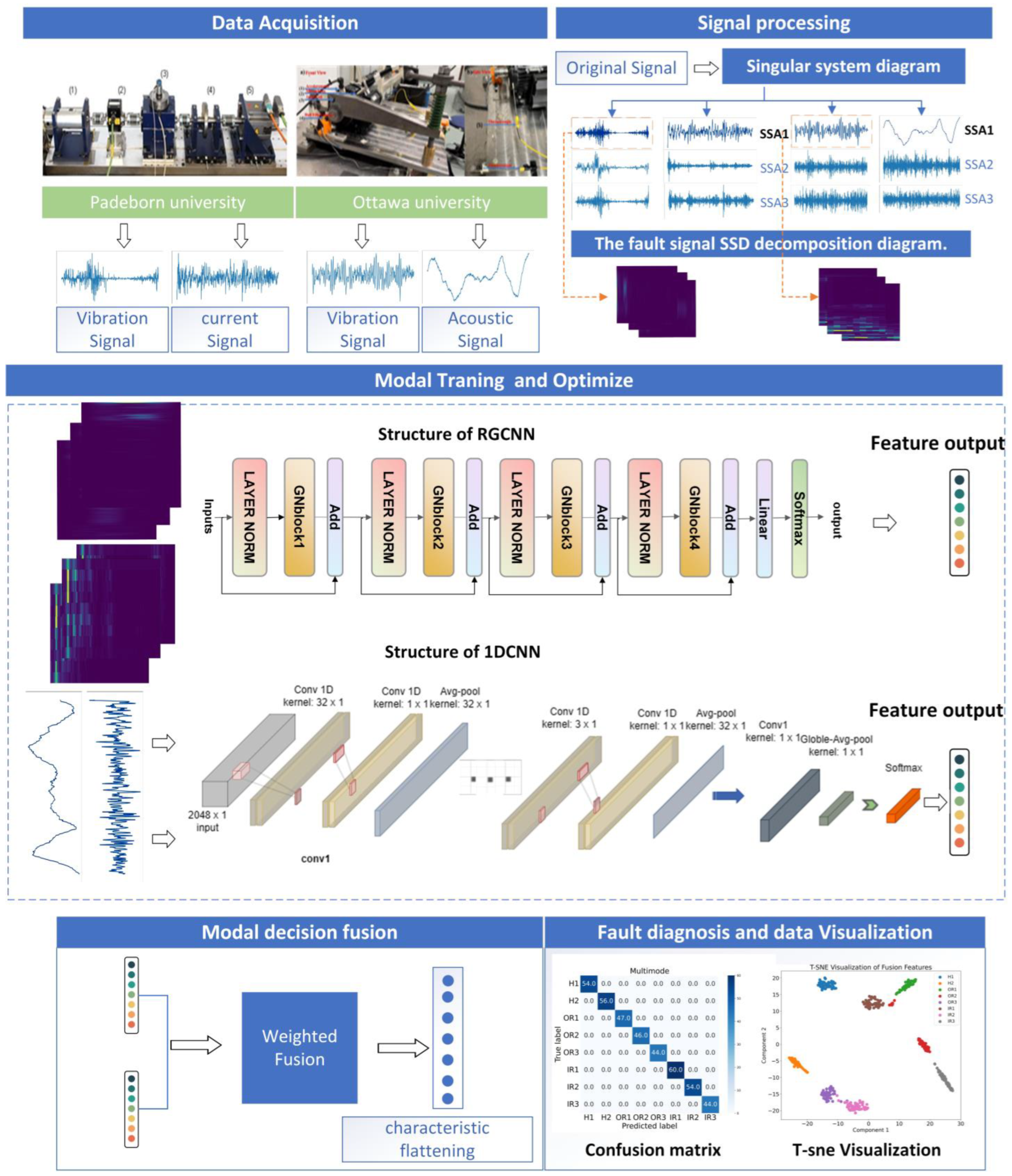
To better represent the fault-related information of vibration and signals, singular spectrum time series analysis is used to extract signal features.

(2)

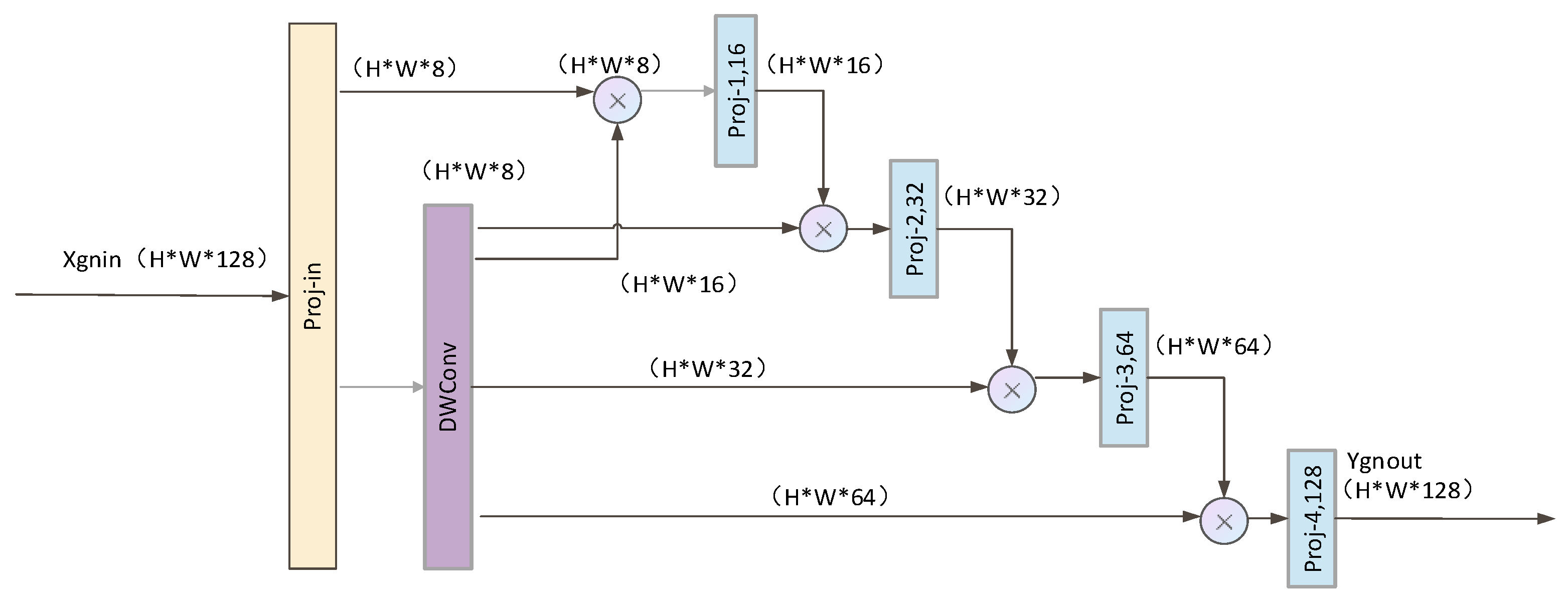
A novel network is constructed using recurrent gated convolution to learn and optimize two-dimensional image data.

(3)

The decision-level fusion method integrates different deep learning models to achieve more accurate fault diagnosis results.

(4)

We conducted experimental evaluations of the proposed method on a dataset of bearings with various faults and performed a comprehensive comparative study.

2. Related Work

Currently, research on fusion methods based on multimodal signals is divided into three main types [27]: data-level fusion, feature-level fusion, and decision-level fusion. The strategy of data-level fusion is to integrate raw data from multiple modalities into a complete dataset using signal processing techniques. This approach usually involves simply splicing or combining data from different modalities through different channels to form fused data [28]. For example, Li et al. [29] and Ma et al. [30] fused acoustic and vibration signals for gearbox fault diagnosis and demonstrated that multi-sensor fusion performs better than single-sensor based methods. The significant advantage of this strategy is the ability to fully utilize the information content of the original data in order to minimize the loss of information during the fusion stage. However, most of the existing data-level fusion techniques simply splice or combine the data collected by different sensors through weighted averaging, which may suffer from insufficient interpretability in interpreting the processing of each sensor’s data.

Feature-level fusion methods first extract signal features from multiple sensors through signal analysis or neural networks and then fuse them by means of feature combination and an attention mechanism to enhance robustness. The multi-layer deep fusion network model proposed by Li achieves adaptive hierarchical fusion by fusing features at different levels through branching and central network structures [31]. Wang proposed a multi-scale, multi-sensor fusion network based on deep learning for motor fault diagnosis [27]. However, feature-level fusion strategies have drawbacks, such as the fact that signal feature acquisition methods that rely on expert experience may limit the robustness and information content of the fused features, and deep learning-based methods may result in missing information by focusing on a limited feature depth.

In implementing a decision-level fusion strategy, the process of information fusion involves integrating decision outcomes from different modal data fusion methods, typically including strategies such as the majority voting fusion strategy, algorithms based on Dempster–Shafer (DS) evidence theory, and their improved versions [32]. These methods exhibit high real-time performance and robustness. Additionally, some researchers have employed a stacked autoencoder using the Morlet wavelet function to extract key features from a series of sensor data and perform classification on these features. To address key issues in multimodal decision fusion, a flexible weighted distribution fusion strategy has been designed, which effectively integrates decision information from different modalities [32]. Given the distinct characteristics of vibration signals and infrared images, Shao et al. [33] proposed a fusion framework based on confidence-weighted support matrix machines, which utilizes DS evidence theory to fuse the posterior probability outputs of different sensor data. Peng et al. [34] proposed a decision-level fusion method using vibration and current signals to identify the three health states of a gearbox. Furthermore, deep learning models have been applied to extract key features from various sensor data, with the decision-level fusion process being carried out using weighted DS evidence theory. Although decision-level fusion strategies demonstrate excellent performance in terms of noise resistance and practicality, their effectiveness largely depends on the fusion strategy employed [35].

3. Methods

To effectively integrate multimodal information and fully leverage its potential in fault diagnosis, this study proposes a novel multimodal fusion fault detection (MFFD) framework, as illustrated in Figure 1. The proposed method consists of four primary modules: a signal processing module, a recurrent gated convolutional neural network (RGCNN) training and optimization module, a one-dimensional convolutional neural network (1DCNN) training module, and a multimodal decision fusion module.

The first step involves acquiring multimodal data from experimental bearings, with singular spectrum analysis techniques employed to extract relevant features. The vibration signals are then processed using the short-time Fourier transform (STFT) [36], generating time–frequency maps, which result in short-time Fourier images and time series samples. The RGCNN is then used to process the time–frequency images, making full use of its ability to capture temporal and spatial correlations in the data. This model effectively extracts fault-related features from the time–frequency domain and is trained to classify fault types based on complex patterns in the input. Simultaneously, the 1DCNN is trained using the time series data to capture the localized temporal features inherent in the vibration signals. This network is well-suited to recognize fault patterns from the sequential nature of the data.

Finally, a multimodal decision fusion module is introduced to combine the outputs of the RGCNN and 1DCNN models. An adaptive weighting strategy is used to assign dynamic weights to each modality based on its diagnostic reliability, ensuring that the complementary strengths of the models are effectively integrated. This fusion enhances both the accuracy and robustness of the fault diagnosis process, allowing for the efficient integration of diverse data sources. The framework’s overall performance is validated in subsequent sections, where each component is discussed in detail.

3.1. Signal Preprocessing Method

Singular spectrum analysis (SSA) is a set of techniques that are widely applicable to a multitude of real-world problems, with applications including, but not being limited to, the fields of classical time series analysis, multivariate statistical analysis, multivariate geometry, dynamical systems research, and signal processing.

The main purpose of SSA is to decompose the original time series into multiple component sequences, each of which can be classified into trend components, periodic components, quasi-periodic components, and noise components. The SSA method consists of two stages and four steps: the decomposition stage, which includes embedding analysis and singular value decomposition; and the reconstruction stage, which is divided into grouping and diagonal averaging. The four steps are as follows:

(1) Embedding: Convert the one-dimensional time series $x_n$ (n = 1, 2, …, N) into a multi-dimensional column vector $x_1$, $x_2$, …, $x_N$, $X_I$ = ($x_1$, …, $x_{i+L-1}$)^T (with T indicating the transpose) for i = 1, 2, …, k. Here, k = N – L + 1, and the embedding parameter L is an integer that satisfies 2 ≤ L ≤ N.

(2) Singular value decomposition (SVD) [37]: The trajectory matrix $X$ is constructed as follows.

$$X=\left[X_1,X_2,\cdots ,X_k\right]=\left[\begin{array}{cccc}{x}_1& x_2& \cdots & x_k\\ x_2& x_3& \cdots & x_{k+1}\\ ⋮& ⋮& \ddots & ⋮\\ x_L& x_{L+1}& \cdots & x_N\end{array}\right]$$

(1)

The matrix $X$ has dimensions L × (N – L + 1), representing the result of the embedding operation. Now, define the covariance matrix Cx = $X^{\mathrm{T}}X$, which is a square matrix of dimensions (N – L + 1) × (N – L + 1) and can be decomposed using eigenvalue decomposition. The eigenvalues are λ₁ ≥ λ₂ ≥ ⋯ ≥ λ_L ≥ 0, and the corresponding eigenvectors form an orthogonal matrix $U$ = ($U_1$, $U_2$, …, $U_L$), called the empirical orthogonal functions (EOFs).

Using singular value decomposition, approximate the matrix $X$ as a sum of rank-1 matrices as follows.

$$X=X_1+X_2+\cdots +X_d={\sum }_{m=1}^d\sum \sqrt{{\lambda }_m}{U}_m{V}_m^{\mathrm{T}}$$

(2)

${\lambda }_m$ is the m-th singular value, and  $U_m$ and $V_m$ are the corresponding eigenvectors. This step represents decomposing the matrix $X$ into the sum of multiple low-rank matrices.

(3) Grouping: In this step, partition the set {1, 2, …, d} into p non-overlapping subsets {I1, …, Ip}. For each subset I, define the composite matrix $X_I$ as follows.

$$X_I=X_{i1}+X_{i2}+\cdots +X_{in}$$

(3)

Thus, the matrix $X$ can be represented as follows.

$$X=X_{I1}+X_{I2}+\cdots +X_{Ip}$$

(4)

(4) Diagonal averaging: Each $X_{Ij}$ (j = 1, 2, …, p) can be transformed into a time series of length N using diagonal averaging.

Let A be an L × K matrix, with elements $a_{ij}$, $1\le i\le \mathrm{L},1\le j\le \mathrm{K},{\mathrm{L}}^{\mathrm{*}}=\mathrm{m}\mathrm{i}\mathrm{n}\{\mathrm{L},\mathrm{K}\},{\mathrm{K}}^{\mathrm{*}}=\mathrm{m}\mathrm{a}\mathrm{x}\{\mathrm{L},\mathrm{K}\}$, and N = L + K − 1. The matrix A can be transformed into the time series $a_1$, …, $a_N$, using the diagonal averaging formula, as follows.

$$a_k=\left\{\begin{array}{ll}{\displaystyle \frac{1}{k}}{\sum }_{p=1}^k{a}_{p,k-p+1}^{\mathrm{*}}& 1⩽k⩽L^{\mathrm{*}}\\ {\displaystyle \frac{1}{L}}{\sum }_{p=1}^{L^{\mathrm{*}}}{a}_{p,k-p+1}^{\mathrm{*}}& L^{\mathrm{*}}⩽k⩽K^{\mathrm{*}}\\ {\displaystyle \frac{1}{T-k+1}}{\sum }_{p=k-K^{\mathrm{*}}+1}^{T-K^{\mathrm{*}}+1}{a}_{p,k-p+1}^{\mathrm{*}}& K^{\mathrm{*}}⩽k⩽N\end{array}\right.$$

(5)

Therefore, for each matrix $X_{Ij}$, using the method described above, a reconstructed sequence can be generated as follows.

$$R{C}_m=({\tilde{x}}_{m,1},\cdots ,{\tilde{x}}_{m,N})$$

(6)

Finally, each reconstructed sequence $R{C}_m$ is generated from each composite matrix $X_{Ij}$, and the original time series can be reconstructed using the following formula.

$$x_n={\sum }_{m=1}^{p}R{C}_{m,n}={\sum }_{m=1}^p{\tilde{x}}_{m,n}n=1,\cdots ,N$$

(7)

This step represents the process of reconstructing the original time series by summing the weighted contributions from the individual components.

To extract relevant features from the original signal, this module employs SSA to perform data denoising, which includes steps such as embedding, singular value decomposition (SVD), grouping, and reconstruction, particularly for vibration signals. Since two-dimensional images encapsulate rich fault-related information, apply the STFT to convert bearing vibration signals into time–frequency representations, which will subsequently be input into the RGCNN model. Similarly, after performing SSA on acoustic or current signals, the resulting one-dimensional signals will be fed into 1DCNN.

3.2. RGCNN Model

In this section, we will introduce the RGCNN and construct a new convolutional neural network based on ${\mathrm{g}}^{\mathrm{n}}\mathrm{C}\mathrm{o}\mathrm{n}\mathrm{v}$ [22].

Before introducing ${\mathrm{g}}^{\mathrm{n}}\mathrm{C}\mathrm{o}\mathrm{n}\mathrm{v}$ and its basic operation gConv, let us first recall the basic convolution operation. The traditional convolution operation for a given input image X ∈ RH × W × C and a convolutional kernel K ∈ RKH × KW × C is defined as follows:

$$Y(t)=(X\mathrm{*}K)(t)={\sum }_{i=1}^{K_H}{\sum }_{j=1}^{K_W}X(t_i,t_j)\cdot K(i,j)$$

(8)

where * denotes the convolution operation, and $Y\in {\mathbb{R}}^{\left(H-K_H+1\right)\times \left(W-K_W+1\right)\times C}$ represents the output feature map.

Building upon this, ${\mathrm{g}}^{\mathrm{n}}\mathrm{C}\mathrm{o}\mathrm{n}\mathrm{v}$ is a generalized convolutional operator capable of capturing higher-order feature interactions and modeling long-range dependencies and has shown effectiveness in downstream image tasks. This paper applies it to upstream image processing tasks. We introduce this module into the convolutional neural network to replace the convolutional layers of conventional convolutional neural networks.

gConv is the basic operation of ${\mathrm{g}}^{\mathrm{n}}\mathrm{C}\mathrm{o}\mathrm{n}\mathrm{v}$ and is considered a first-order interaction. Given the input features ${\mathrm{X}}_{\mathrm{g}\mathrm{i}\mathrm{n}}\in {\mathbb{R}}^{\mathrm{H}\times \mathrm{W}\times \mathrm{C}}$, the resulting features ${\mathrm{Y}}_{\mathrm{g}\mathrm{o}\mathrm{u}\mathrm{t}}$ from gConv can be computed using Equation (5).

$$\begin{array}{l}[P_0,Q_0]=F_{\mathrm{P}\mathrm{r}\mathrm{o}\mathrm{j}-\mathrm{i}\mathrm{n}}\left(X_{g\mathrm{i}\mathrm{n}}\right)\\ P_1=DWConv\left(Q_0\right)\otimes P_0\\ Y_{g\mathrm{out}}=F_{\mathrm{Proj}-\mathrm{out}}(P_1)\end{array}$$

(9)

In this context, $F_{Proj-in}\left(\cdot \right)$ and $F_{Proj-out}(\cdot )$ represent the input linear projection layer and the output linear projection layer of gConv, respectively; while $\mathrm{D}\mathrm{W}\mathrm{C}\mathrm{o}\mathrm{n}\mathrm{v}(\cdot )$ denotes the depthwise convolution layer operation. In gConv, the input features $X_{\mathrm{g}\mathrm{i}\mathrm{n}}$ are projected to ${\mathsf{P}}_0,{\mathsf{Q}}_0({\mathsf{P}}_0,{\mathsf{Q}}_0\in {\mathbb{R}}^{\mathsf{H}\times \mathsf{W}\times \mathsf{C}})$. The depthwise convolution is used to capture long-range dependencies and achieve single interactions between adjacent features through element-wise multiplication.

The recursive gated convolution ${\mathrm{g}}^{\mathrm{n}}\mathrm{C}\mathrm{o}\mathrm{n}\mathrm{v}$ was designed based on gConv to introduce higher-order interactions. To prevent excessive computational overhead from these higher-order interactions, the number of channels involved in each order of computation is set to a lower count, with fewer channels used for lower-order interactions. Given the input features $X_{\mathrm{g}\mathrm{n}\mathrm{i}\mathrm{n}}\in {\mathbb{R}}^{\mathrm{H}\times \mathrm{W}\times \mathrm{C}}$, the resulting features from ${\mathrm{g}}^{\mathrm{n}}\mathrm{C}\mathrm{o}\mathrm{n}\mathrm{v}$ can be computed using Equation (7).

$$\begin{array}{l}[P_0,Q_0,Q_1,\cdots ,Q_{n-1}]=F_{\mathrm{P}\mathrm{r}\mathrm{o}\mathrm{j}-\mathrm{i}\mathrm{n}}\left(X_{gn\mathrm{i}\mathrm{n}}\right)\\ P_1=DWConv\left(Q_0\right)\otimes P_0/\alpha \\ P_{k+1}=DWConv\left(Q_k\right)\otimes F_{Proj\cdot k}\left(P_k\right)/\alpha \\ (Q_k\in Q_0,Q_1,\cdots ,Q_{n-1})\\ Y_{gn\mathrm{o}\mathrm{u}\mathrm{t}}=F_{\mathrm{P}\mathrm{r}\mathrm{o}\mathrm{j}-\mathrm{o}\mathrm{u}\mathrm{t}}\left(P_n\right)\end{array}$$

(10)

In this context, $F_{Proj-k}(\cdot )$ represents the linear projection layer used to adjust the number of P channels after the k-th (k = 1, 2, …, n − 1) order of interaction. The coefficient 1/α is used to scale the output.

The network structure of ${\mathrm{g}}^4\mathrm{C}\mathrm{o}\mathrm{n}\mathrm{v}$ is outlined in the Figure 2. ${\mathrm{g}}^4\mathrm{C}\mathrm{o}\mathrm{n}\mathrm{v}$ is designed to realize arbitrary-order spatial interactions through a highly efficient implementation that leverages gated convolutions and recursive design principles. To enhance its performance, we construct the GNblock module to replace the convolution layers of convolutional neural networks, followed by normalization layers, and then output feature vectors through a multilayer perceptron (MLP), which is somewhat similar to the self-attention mechanism. Additionally, the network incorporates the input adaptive interaction characteristics of gated convolution, allowing the recursive gated convolution module to extract deeper features through higher-order spatial interactions. This unique gated mechanism effectively captures spatiotemporal features in time–frequency maps, enabling the network to retain key features while effectively reducing noise interference. The constructed network structure is illustrated in the framework diagram.

3.3. 1DCNN Model

For the one-dimensional time series signals of the bearings, in order to effectively extract features from the time-domain data, we constructed a 1DCNN model. This model utilizes successive convolutional layers and pooling layers to effectively identify and extract key features from the time series data.

To ensure that the complete periodic signal data are covered in the input signal samples, the length of the input signal samples of the 1DCNN is set to 2048 × 1. In 1DCNN, we use stride convolution instead of max pooling to aggregate feature information and reduce the feature dimension without losing information. We employ a diverse set of convolutional kernels in the network to process the network input signal in order to learn its long and short-term features in depth. The number of convolutional channels in the convolutional layer directly affects the number of features that can be learnt and extracted. Specific parameters are detailed in

Table 1. Network configuration of The 1DCNN architecture.

Layer	Type	Kernel	Channel	Stride	Pading	OUTPUT
1	INPUT	-	-	-	-	2048 × 1
2	Conv	32 × 1	32	1	Yes	2048 × 32
3	Conv	1 × 1	32	-	Yes	2048 × 32
4	AVP	32 × 1	-	-	-	2048 × 32
5	Conv	16 × 1	32	2	Yes	1024 × 32
6	Conv	1 × 1	32	-	Yes	1024 × 32
7	AVP	32 × 1	-	-	-	1024 × 32
8	Conv	9 × 1	64	2	Yes	512 × 64
9	Conv	1 × 1	64	-	Yes	512 × 64
10	AVP	32 × 1	-	-	-	512 × 64
11	Conv	6 × 1	64	2	Yes	256 × 64
12	Conv	1 × 1	64	-	Yes	256 × 64
13	AVP	32 × 1	-	-	-	256 × 64
14	Conv	3 × 1	128	4	Yes	64 × 128
15	Conv	1 × 1	128	-	Yes	64 × 128
16	AVP	32 × 1	-	-	-	64 × 128
17	Conv	3 × 1	128	4	Yes	16 × 128
Global AVP
SoftMax

.

3.4. Multimodal Fusion for Decision-Making

STFT image samples and time series samples are fed into RGCNN and 1DCNN, respectively. Both neural networks are trained simultaneously, and the model parameters are optimized to obtain a basic classifier for rolling bearing fault diagnosis. Comprehensive fault diagnosis results can be achieved through multimodal decision fusion, which is implemented by integrating multiple different deep learning models.

The output features from the two networks are integrated using a weighted fusion strategy. We employ an adaptive weight adjustment mechanism to dynamically adjust the weights based on the importance of different modal features. This strategy ensures that the features from each modality are appropriately considered in the final classification decision.

The two feature vectors, F1 and F2, come from the two networks. We aim to obtain a fused feature vector F through a weighted fusion strategy. We can express F as follows.

$$\mathrm{F}=\mathsf{\alpha }\mathrm{F}1+(1-\mathsf{\alpha })\mathrm{F}2$$

(11)

α is a weight that represents the importance of the first feature vector F1 in the fused feature vector F. To enable the adaptive adjustment of α, we can implement an adaptive weight adjustment mechanism. This mechanism dynamically adjusts α based on the importance of different modal features.

Assume we have a loss function L that represents the performance of the fused feature vector F in the classification task. We can optimize the weight α using gradient descent to minimize the loss function L. Specifically, we can update α through gradient updating as follows.

$$\mathsf{\alpha }=\mathsf{\alpha }-\mathsf{\lambda }\partial \mathrm{L}/\partial \mathsf{\alpha }$$

(12)

λ is the learning rate, which is used to control the rate at which the weights are updated. In this way, α can be automatically adjusted according to the changes in the loss function L, ensuring that the features of each modality receive appropriate attention in the final classification decision.

$$\mathrm{P}\left(\mathrm{x}\right)=\mathrm{a}\mathrm{r}\mathrm{g}\mathrm{m}\mathrm{a}\mathrm{x}\left(\alpha \mathrm{F}1+\left(1-\alpha \right)\mathrm{F}2\right)/2$$

(13)

4. Results

4.1. Dataset

The Ottawa University rolling bearing dataset [38], known as the UORED-VAFCLS (vibration and acoustic fault characteristics under constant load and speed), is collected under constant load and speed conditions using a test bench, referred to as the Ottawa dataset. This dataset includes vibration and acoustic fault characteristic data for rolling element bearings operating under stable nominal rotational speeds and loads. Each group of raw data is obtained at these constant conditions, as shown in Figure 3.

The dataset covers four different failure types: inner raceway, outer raceway, ball, and cage, with five instances of each failure type. The Ottawa dataset is dedicated to the 6203 deep groove ball bearing with a sampling frequency of 48 kHz. The collected data consist of both vibration signal data and acoustic signal data. The parameters of the selected bearing dataset are shown in the following

Table 2. Operating parameters of Ottawa bearings.

Bearing Code	Bearing Name	Damage Level	Class	Characteristic of Damage
H-1-0	H1	No damage	H	Single point
I-1-2	IR1	No damage	IR	Single point
0-6-2	OR1	Plasticdeform; indentations	OR	Single point
B-11-2	B1	Fatigue; pitting	B	Single point
C-16-2	C1	Plasticdeform	C	Single point

H: healthy; IR: inner race defect; OR: outer race defect; C: cage defect; B: ball defect.

.

In addition to utilizing the Ottawa bearing dataset, experimental data obtained from the Pade bearing test bed at the University of Paderborn was adopted for the performance validation process [39]. As shown in Figure 4, the Pade bearing test bench consists of a motor, a torque measuring shaft, a rolling bearing test module, a flywheel, and a load motor. In order to effectively monitor the operational status of the bearings, the dataset was comprehensively evaluated by measuring the phase currents of the drive motor, as well as the acceleration of the bearing housing. In this experiment, the test bearing used was a model 6203, whose operating parameters included a shaft speed of 1500 r/min, a radial force of 1000 N, and a load torque of 0.7 N m, all of which were kept constant.

The bearing measurements contained in the Pade dataset are classified into three main categories: normal, inner raceway failures, and outer raceway failures. Further, depending on the degree of damage caused by the faults, it is possible to categorize these faults into two classes: the first class is for those cases where the damage is minor, i.e., those where the damage diameter is less than 2 mm; the second class covers faults where the damage diameter is between 2 mm and 4.5 mm. In addition, the raw accelerometer measurements were taken at a high sampling frequency of 64 kHz.

In this study, we use the fault classification data from this bearing dataset to validate model performance. Vibration and current data from eight bearings, coded as K001, KA01, KI01, etc., are selected for the dataset. The parameters of the selected bearing dataset are shown in the following

Table 3. Operating parameters of Paderborn bearings.

Bearing Code	Bearing Name	Damage	Class	Characteristic of Damage
K001	H1	No damage	H	-
K002	H2	No damage	H	-
KA15	OR1	Plasticdeform; indentations	OR	Single point
KA16	OR2	Fatigue; pitting	OR	Single point
KA30	OR3	Plasticdeform; indentations	OR	Distributed
KI16	IR1	Fatigue; pitting	IR	Single point
KI18	IR2	Fatigue; pitting	IR	Single point
KI21	IR3	Fatigue; pitting	IR	Single point

IR: inner race defect; OR: outer race defect; H: healthy.

4.2. Parameter Settings

The simulation environment in this study was established using the Python 3.9 programming language and the deep learning framework PyTorch 1.12.0. The configuration of the simulation platform includes a 13th Gen Intel(R) Core(TM) i5-12400H processor running at 2.50 GHz, 16 GB of memory, a GTX 4060 GPU, and the Windows 11 64-bit operating system.

Before training, the dataset was divided into training and testing sets with a ratio of 7:3. During training, the batch size was set to 32. A decaying learning rate was applied throughout the training process, with an initial learning rate of 0.05. The number of iterations was set to 20, and the Adam optimizer was utilized for model training, with the initial setting of α1 set to 0.5, which assumes equal importance for all features initially. This balanced choice prevents biasing the model toward any particular feature at the start of training.

4.3. Fault Detection Results Analysis

To assess the effectiveness of the proposed multimodal decision fusion diagnostic method for rolling bearing fault detection, various tests were conducted. The output results are presented in a confusion matrix, which includes different classification performance metrics, such as accuracy, recall, and F1 score. The confusion matrix displays each class with a corresponding row and column. Each entry in the confusion matrix indicates the number of test samples, where the columns represent the true classes, and the rows represent the predicted classes.

Initially, the performance of each modality model was analyzed on the Ottawa and Pade datasets, and a comparison was made with the proposed multimodal decision fusion method.

4.4. Fault Diagnosis Based on Individual Modes

To clearly highlight the advantages of the MFFD model in the context of single modalities, corresponding time-domain and time–frequency-domain models were developed. Following the signal processing phase, the fault detection methods were validated across different datasets. Specifically, for the Ottawa and Pade datasets, vibration signals were utilized as input for the image modality, while acoustic signals were employed for the time series modality. In the case of the Paderborn dataset, vibration signals were used for the image modality, and current signals were used for the time series modality. All operations were conducted under consistent data preprocessing conditions. The performance of the baseline models for single modalities was compared to that of the multimodal approach in bearing fault diagnosis. The detailed baseline methods and experimental results are provided in

Table 4. Results of comparisons using different methods.

Dataset	Ottawa			Pade
Method	1DCNN	RGCNN	MFFD	1DCNN	RGCNN	MFFD
Accuracy	89.25	95.75	98.75	92.25	96.00	99.00
Precision	0.9012	0.9590	0.9887	0.9255	0. 9624	0.0991
Recall	0.8998	0.9562	0.9871	0.9240	0. 9590	0.9898
F1	0.8992	0.9569	0.9877	0.9231	0.9598	0.9903

.

In the fault diagnosis based on image signals, the processed bearing vibration signals were input into the RGCNN model for training. After 20 training epochs, classification prediction results were obtained. The confusion matrix are shown in Figure 5. The network’s error gradually decreased with the increase in epochs, and after 20 epochs, the network converged, achieving an accuracy of 95.75% and 96.00%.

For the fault diagnosis based on time series signals, the processed time series signals were input into the 1DCNN model for training. After 20 training epochs, classification prediction results were obtained, and the training convergence curve of the network is illustrated in Figure 7. Similar to the previous model, the network’s error decreased over the epochs, and after 20 epochs, the network converged, achieving accuracies of 89.25% and 92.25%, respectively.

To demonstrate the effectiveness of the proposed method, 10 repeated experiments were conducted. Additionally, confusion matrix and T-SNE visualizations were performed, as shown in Figure 5 and Figure 6. These visualizations intuitively illustrate the classification performance of the proposed model.

4.5. Fault Diagnosis Method Based on MFFD

In this section, we used the MFFD method to train the processed image signals and time series signals. In order to validate the practicality of the proposed method, we repeat the experiments 10 times and calculate the accuracy of the method on the Paderborn and Ottawa datasets, respectively. Figure 7 shows the convergence curves of the network during the training process. As can be seen from Figure 7, the network completely converges after 20 epochs, and the accuracy reaches 98.75% and 99.00%, respectively.

In addition, the performance of the proposed method can be demonstrated more intuitively by observing the confusion matrix analysis and T-SNE visualization, as shown in Figure 5 and Figure 6. With the T-SNE method, we can clearly observe the difference between different categories of samples, which proves the superiority of the proposed signal processing method. Moreover, the highest diagnostic accuracy of the multimodal approach achieves the best results in both datasets, reaching 98.75% and 99.00%, which is significantly better than the single-modal results. This further validates the effectiveness of multimodal signal fusion and reflects the robustness and stability of our method.

4.6. Ablation Study of Singular Spectrum Analysis

The core objective of this section is to explore the application value of singular spectrum time series reconstruction technology in the field of signal processing and the potential impact of this technology. Through this research, we provide a detailed overview of how to utilize this technique to extract the key temporal features of signals and employ an ablation study approach to systematically validate the effectiveness of the technology. To enhance the persuasiveness of the study, we introduce practical case analyses and support our findings with experimental data, demonstrating the performance of this technology across different datasets.

The experimental results show that the introduction of the SSA technique significantly improves the fault diagnosis accuracy in both the Paderborn bearing dataset and the Ottawa bearing dataset. As shown in Figure 8, the accuracy of the RGCNN method reaches 95.00% and 94.00% when testing different datasets containing different faults, respectively. However, after applying the singular spectrum time series reconstruction technique, the accuracy increases to 95.75% and 96.00%, and the 1DCNN method achieves 85.75% and 89.00%, respectively. However, after applying the singular spectrum time series reconstruction technique, the accuracy is improved to 89.25% and 92.25%. The accuracy of MFFD method is also improved by 1.75% and 0.60%, respectively.

The outcomes of the various comparative experiments effectively validate that the introduction of SSA significantly enhances identification accuracy and contributes to the stability of the model. In other words, SSA can effectively focus on the essential characteristics of multimodal information, thereby achieving the established objectives.

4.7. Ablation Study of Order n for High Order Interactions

The selection of the order in recursive gated convolution (${\mathrm{g}}^{\mathrm{n}}\mathrm{C}\mathrm{o}\mathrm{n}\mathrm{v}$) is critical. By configuring different orders, the model can extract deeper features through spatial interactions at various levels, effectively capturing spatiotemporal characteristics in time–frequency representations. This capability allows the network to retain essential features while significantly reducing noise interference, thereby obtaining feature information across multiple scales.

To validate the effectiveness of the recursive gated convolution, we examined the model’s diagnostic performance by varying the order n. All other experimental parameters were kept constant, with only the size of n altered. We repeated the experiments ten times on both the Pade and Ottawa datasets, calculating the average results. The experimental outcomes are presented in Figure 9. Analysis reveals that when n = 4, the model achieves the best performance, with an average accuracy of 95.75% and 96.00%. Therefore, this study selects a dilation rate of n = 4 for the recursive gated convolution.

4.8. Comparison of Other Methods

This section discusses the advantages of the multimodal fusion fault diagnosis method based on SSA over other related approaches. To better illustrate the accuracy and advantages of the proposed diagnostic approach for bearing fault diagnosis, we compared its performance with existing methods under the same data preprocessing conditions. As shown in

Table 5. Comparison with different models.

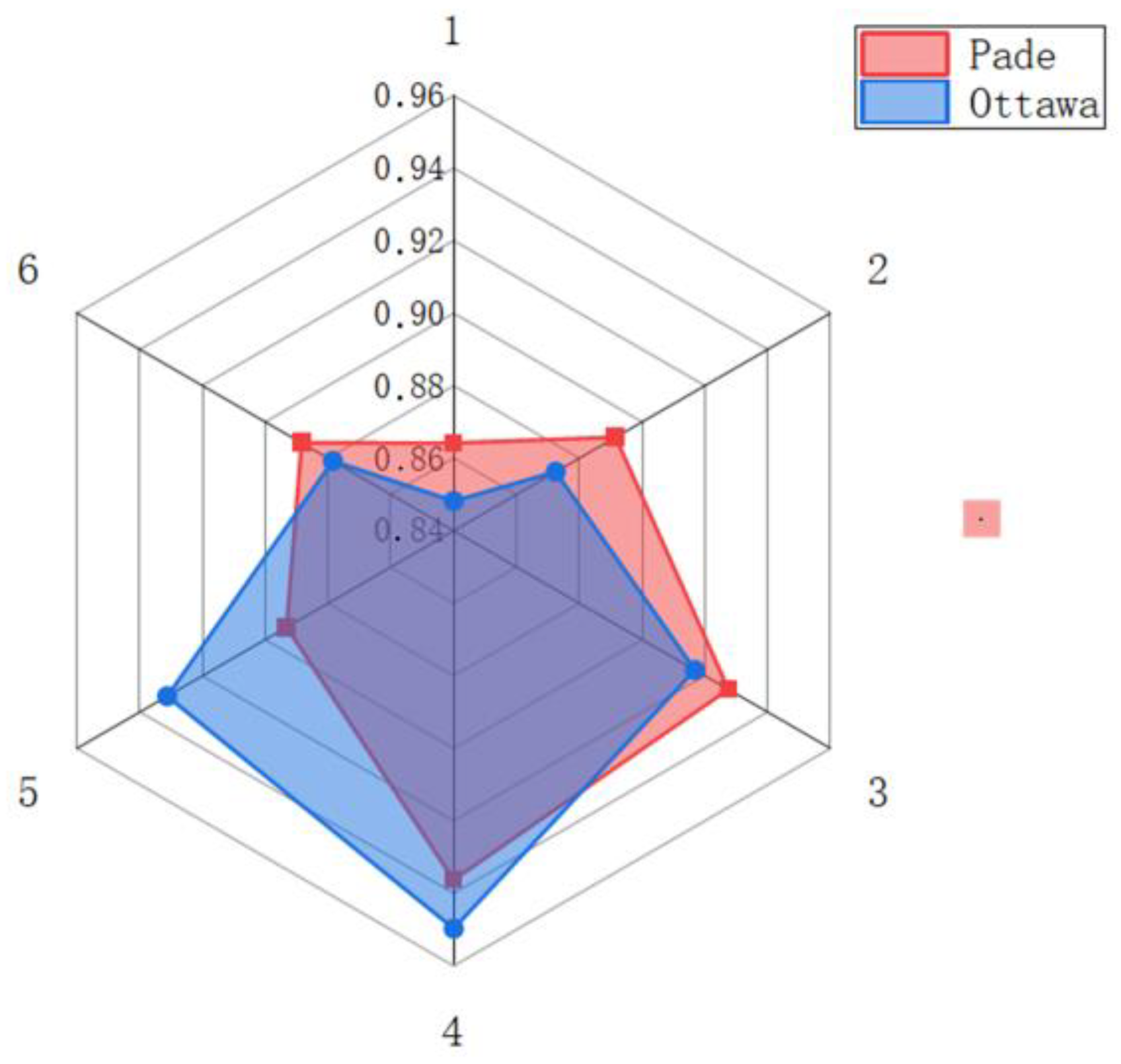
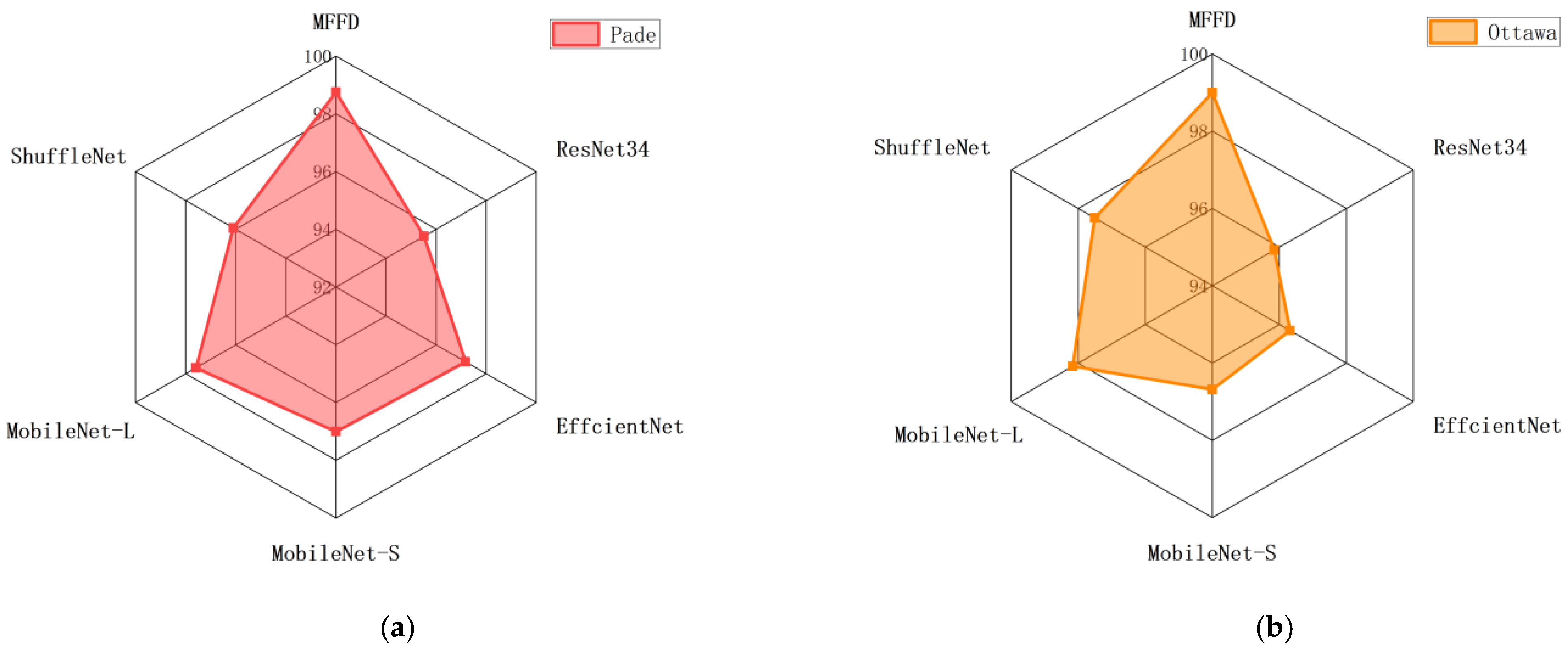
Dataset	Pade						Ottawa
Method	ResNet34	Effcient Net	Mobile Net-S	Mobile Net-L	Shuffle Net	MFFD	ResNet34	Effcient Net	Mobile Net-S	Mobile Net-L	Shuffle Net	MFFD
Accuracy	95.52	97.18	97.01	97.59	96.10	98.75	95.85	96.32	96.68	98.17	97.51	99.00
Precision	0.9586	0.9722	0.9702	0.9763	0.9627	0.9887	0.9600	0.9629	0.9685	0.9821	0.9753	0.9910
Recall	0.9554	0.9733	0.9710	0.9755	0.9609	0.9871	0.9590	0.9733	0.9667	0.9816	0.9744	0.9898
F1	0.9554	0.9718	0.9698	0.9752	0.9609	0.9877	0.9584	0.9632	0.9667	0.9816	0.9747	0.9903

and the Figure 10, we evaluated the proposed method against five state-of-the-art models: ResNet34, MobileNet-S, MobileNet-L, ShuffleNet, and EfficientNet. The diagnostic accuracies of the other methods are lower than those of the proposed method on both the Paderborn and the Ottawa datasets, with our approach achieving accuracies of 98.75% and 99.00%, respectively.

This demonstrates that our method not only outperforms traditional unimodal methods in terms of accuracy but also excels in recall and overall performance. The radar chart further highlights the superior fault recognition capabilities of the proposed multimodal method in identifying fault types, showcasing its advantages over the other models.

5. Conclusions

In this paper, we propose a novel method combining deep learning and multimodal fusion to achieve the robust and accurate fault diagnosis of rolling bearings. The method first extracts essential features from multimodal data through singular spectrum analysis (SSA) then uses different deep learning models to classify data from various modalities. Finally, decision-level multimodal fusion is applied to integrate the outputs of these models, yielding comprehensive and reliable fault diagnosis results.

The innovation of our approach lies in its ability to effectively handle and fuse multimodal data, including short-time Fourier images and time series data, using deep learning models. By utilizing recursive gated convolutional neural networks (RGCNNs) and 1D convolutional neural networks (1DCNNs) as base models, we are able to achieve superior fault classification accuracy compared to conventional methods. Additionally, the decision-level multimodal fusion method based on weighted average fusion optimizes the contributions of both the samples and models, producing a more reliable and accurate diagnosis through weighted voting.

Through extensive case analysis of a rolling bearing dataset containing various fault types, we have demonstrated that the proposed method outperforms both individual deep learning models and traditional methods in terms of fault diagnosis accuracy. This improvement is largely due to the integration of multiple deep learning models and the decision-level fusion, which, together, enhance the robustness and accuracy of the diagnostic results.

In the future, we plan to expand the scope of this method by incorporating additional time-domain and frequency-domain features for fault diagnosis, as well as exploring its application across the entire lifecycle of rolling bearings, including early-, mid-, and late-stage faults. Furthermore, enhancing the robustness and generalization of the proposed method under different operating conditions will be a critical area of future research.

References

- Jia, N.; Huang, W.; Ding, C.; Wang, J.; Zhu, Z. Physics-informed unsupervised domain adaptation framework for cross-machine bearing fault diagnosis. Adv. Eng. Inform. 2024, 62, 102774. [Google Scholar] [CrossRef]
- Cui, B.; Cheng, Y.; Jia, P.; Liu, Z.; Wang, B.; Ye, J.; Li, Y.; Chen, W.; Wang, Z. Temperature Field Analysis and Temperature Control of Vacuum Ultra High Speed Angular Contact Ball Bearings. J. Phys. Conf. Ser. 2024, 2784, 012009. [Google Scholar] [CrossRef]
- Sheng, L.; Qiubo, J.; Yadong, X.; Ke, F.; Yulin, W.; Beibei, S.; Xiaoan, Y.; Xin, S.; Ke, Z.; Qing, N. Digital twin-driven focal modulation-based convolutional network for intelligent fault diagnosis. Reliab. Eng. Syst. Saf. 2023, 240, 109590. [Google Scholar] [CrossRef]
- Lu, F.; Tong, Q.; Jiang, X.; Feng, Z.; Liu, R.; Xu, J.; Huo, J. DPICEN: Deep physical information consistency embedded network for bearing fault diagnosis under unknown domain. Reliab. Eng. Syst. Saf. 2024, 252, 110454. [Google Scholar] [CrossRef]
- Lu, Y.; Li, Q.; Liang, S.Y. Physics-based intelligent prognosis for rolling bearing with fault feature extraction. Int. J. Adv. Manuf. Technol. 2018, 97, 611–620. [Google Scholar] [CrossRef]
- Zhao, D.; Shao, D.; Cui, L. CTNet: A data-driven time-frequency technique for wind turbines fault diagnosis under time-varying speeds. ISA Trans. 2024, 154, 335–351. [Google Scholar] [CrossRef]
- Li, Y.; Wang, T.; Xie, J.; Yang, J.; Pan, T.; Yang, B. A simulation data-driven semi-supervised framework based on MK-KNN graph and ESSGAT for bearing fault diagnosis. ISA Trans. 2024, 155, 261–273. [Google Scholar] [CrossRef]
- Hu, Y.; Li, H.; Shi, P.; Chai, Z. A prediction method for the real-time remaining useful life of wind turbine bearings based on the Wiener process. Renew. Energy 2018, 127, 452–460. [Google Scholar] [CrossRef]
- Wan, W.; Chen, J.; Xie, J. MIM-Graph: A multi-sensor network approach for fault diagnosis of HSR Bogie bearings at the IoT edge via mutual information maximization. ISA Trans. 2023, 139, 574–585. [Google Scholar] [CrossRef]
- Pan, Z.; Guan, Y.; Fan, F.; Zheng, Y.; Lin, Z.; Meng, Z. Rolling bearings fault diagnosis based on two-stage signal fusion and deep multi-scale multi-sensor network. ISA Trans. 2024, 154, 311–334. [Google Scholar] [CrossRef]
- Cheng, Y.; Lin, M.; Wu, J.; Zhu, H.; Shao, X. Intelligent fault diagnosis of rotating machinery based on continuous wavelet transform-local binary convolutional neural network. Knowl. -Based Syst. 2021, 216, 106796. [Google Scholar] [CrossRef]
- Liu, Y.; Wen, W.; Bai, Y.; Meng, Q. Self-supervised feature extraction via time–frequency contrast for intelligent fault diagnosis of rotating machinery. Measurement 2023, 210, 112551. [Google Scholar] [CrossRef]
- Zhang, J.; Zhang, Q.; Qin, X.; Sun, Y. A two-stage fault diagnosis methodology for rotating machinery combining optimized support vector data description and optimized support vector machine. Measurement 2022, 200, 111651. [Google Scholar] [CrossRef]
- Wei, H.; Zhang, Q.; Shang, M.; Gu, Y. Extreme learning Machine-based classifier for fault diagnosis of rotating Machinery using a residual network and continuous wavelet transform. Measurement 2021, 183, 109864. [Google Scholar] [CrossRef]
- Zhang, D.; Stewart, E.; Ye, J.; Entezami, M.; Roberts, C. Roller bearing degradation assessment based on a deep MLP convolution neural network considering outlier regions. IEEE Trans. Instrum. Meas. 2019, 69, 2996–3004. [Google Scholar] [CrossRef]
- Zhilin, D.; Dezun, Z.; Lingli, C. An intelligent bearing fault diagnosis framework: One-dimensional improved self-attention-enhanced CNN and empirical wavelet transform. Nonlinear Dyn. 2024, 112, 6439–6459. [Google Scholar]
- Li, F.; Wang, L.; Wang, D.; Wu, J.; Zhao, H. An adaptive multiscale fully convolutional network for bearing fault diagnosis under noisy environments. Measurement 2023, 216, 112993. [Google Scholar] [CrossRef]
- Zhang, Z.; Wu, L. Graph neural network-based bearing fault diagnosis using Granger causality test. Expert Syst. Appl. 2024, 242, 122827. [Google Scholar] [CrossRef]
- Shao, Y.; Yuan, X.; Zhang, C.; Song, Y.; Xu, Q. A novel fault diagnosis algorithm for rolling bearings based on one-dimensional convolutional neural network and INPSO-SVM. Appl. Sci. 2020, 10, 4303. [Google Scholar] [CrossRef]
- Ince, T.; Kiranyaz, S.; Eren, L.; Askar, M.; Gabbouj, M. Real-time motor fault detection by 1-D convolutional neural networks. IEEE Trans. Ind. Electron. 2016, 63, 7067–7075. [Google Scholar] [CrossRef]
- He, K.; Zhang, X.; Ren, S.; Sun, J. Deep residual learning for image recognition. In Proceedings of the IEEE Conference on Computer Vision and Pattern Recognition, Las Vegas, NV, USA, 27–30 June 2016; pp. 770–778. [Google Scholar]
- Rao, Y.; Zhao, W.; Tang, Y.; Zhou, J.; Lim, S.N.; Lu, J. Hornet: Efficient high-order spatial interactions with recursive gated convolutions. arXiv 2022, 35, 10353–10366. [Google Scholar]
- Luo, Y.; Lu, W.; Kang, S.; Tian, X.; Kang, X.; Sun, F. Enhanced Feature Extraction Network Based on Acoustic Signal Feature Learning for Bearing Fault Diagnosis. Sensors 2023, 23, 8703. [Google Scholar] [CrossRef] [PubMed]
- Kundu, P. Review of rotating machinery elements condition monitoring using acoustic emission signal. Expert Syst. Appl. 2024, 252, 124169. [Google Scholar] [CrossRef]
- Bonizzi, P.; Karel, J.M.; Meste, O.; Peeters, R.L. Singular spectrum decomposition: A new method for time series decomposition. Adv. Adapt. Data Anal. 2014, 6, 1450011. [Google Scholar] [CrossRef]
- Lin, T.; Ren, Z.; Zhu, L.; Huang, K.; Zhu, Y.; Zeng, L.; Wan, J. Neural architecture search for multi-sensor information fusion-based intelligent fault diagnosis. Adv. Eng. Inform. 2024, 62, 102776. [Google Scholar] [CrossRef]
- Wang, J.; Fu, P.; Zhang, L.; Gao, R.X.; Zhao, R. Multilevel information fusion for induction motor fault diagnosis. IEEE/ASME Trans. Mechatron. 2019, 24, 2139–2150. [Google Scholar] [CrossRef]
- Xia, M.; Li, T.; Xu, L.; Liu, L.; De Silva, C.W. Fault diagnosis for rotating machinery using multiple sensors and convolutional neural networks. IEEE/ASME Trans. Mechatron. 2017, 23, 101–110. [Google Scholar] [CrossRef]
- Li, C.; Sanchez, R.-V.; Zurita, G.; Cerrada, M.; Cabrera, D.; Vásquez, R.E. Gearbox fault diagnosis based on deep random forest fusion of acoustic and vibratory signals. Mech. Syst. Signal Process. 2016, 76, 283–293. [Google Scholar] [CrossRef]
- Ma, M.; Sun, C.; Chen, X. Deep coupling autoencoder for fault diagnosis with multimodal sensory data. IEEE Trans. Ind. Inform. 2018, 14, 1137–1145. [Google Scholar] [CrossRef]
- Li, X.; Wan, S.; Liu, S.; Zhang, Y.; Hong, J.; Wang, D. Bearing fault diagnosis method based on attention mechanism and multilayer fusion network. ISA Trans. 2022, 128, 550–564. [Google Scholar] [CrossRef]
- Shao, H.; Lin, J.; Zhang, L.; Galar, D.; Kumar, U. A novel approach of multisensory fusion to collaborative fault diagnosis in maintenance. Inf. Fusion 2021, 74, 65–76. [Google Scholar] [CrossRef]
- Li, X.; Cheng, J.; Shao, H.; Liu, K.; Cai, B. A fusion CWSMM-based framework for rotating machinery fault diagnosis under strong interference and imbalanced case. IEEE Trans. Ind. Inform. 2021, 18, 5180–5189. [Google Scholar] [CrossRef]
- Peng, Y.; Qiao, W.; Cheng, F.; Qu, L. Wind turbine drivetrain gearbox fault diagnosis using information fusion on vibration and current signals. IEEE Trans. Instrum. Meas. 2021, 70, 3518011. [Google Scholar] [CrossRef]
- Huo, Z.; Martínez-García, M.; Zhang, Y.; Shu, L. A multisensor information fusion method for high-reliability fault diagnosis of rotating machinery. IEEE Trans. Instrum. Meas. 2021, 71, 3500412. [Google Scholar] [CrossRef]
- Wang, W.; McFadden, P. Early detection of gear failure by vibration analysis i. calculation of the time-frequency distribution. Mech. Syst. Signal Process. 1993, 7, 193–203. [Google Scholar] [CrossRef]
- Golyandina, N.; Nekrutkin, V.; Zhigljavsky, A.A. Analysis of Time Series Structure: SSA and Related Techniques; CRC Press: Boca Raton, FL, USA, 2001. [Google Scholar]
- Sehri, M.; Dumond, P.; Bouchard, M. University of Ottawa constant load and speed rolling-element bearing vibration and acoustic fault signature datasets. Data Brief 2023, 49, 109327. [Google Scholar] [CrossRef]
- Lessmeier, C.; Kimotho, J.K.; Zimmer, D.; Sextro, W. Condition monitoring of bearing damage in electromechanical drive systems by using motor current signals of electric motors: A benchmark data set for data-driven classification. In Proceedings of the PHM Society European Conference, Bilbao, Spain, 5–8 July 2016. [Google Scholar] [CrossRef]