Two-Dimensional Vortex Solitons in Spin-Orbit-Coupled Dipolar Bose–Einstein Condensates

Abstract

Solitons are self-trapped modes existing in various nonlinear systems. Creating stable solitons in two- and three-dimensional settings is a challenging goal in various branches of physics. Several methods have been developed theoretically and experimentally to achieve this, but few of them can support stable multi-dimensional solitons in free space. Recently, a new scheme using spin-orbit-coupling (SOC) has been proposed to create stable 2D solitons in Bose–Einstein condensates (BECs). This paper reviews recent theoretical progress on creating stable 2D solitons in spinor dipolar BEC with SOC, combined with long-range dipole-dipole interaction (DDI), Zeeman splitting (ZS) and contact nonlinearity, in free space. The continuous family of stable symmetric vortex solitons (SVS), asymmetric vortex solitons (AVS), as well as gap solitons (GS) is found via different settings. Their existence and stability conditions are summarized and discussed in detail. The mobility properties of these types of solitons are also addressed. For SVS, a potential method to manipulate its shape and mobility is investigated. These results are supposed to enrich our understanding of 2D solitons and help create multi-dimensional solitons in experiments.

1. Introduction

Creating stable solitons or self-trapped modes in systems with a dimension higher than one remains a challenging and attractive problem in physics, both in theory and experiments [1,2]. The main obstacle lies in the ubiquitous cubic nonlinearity, which could be the Kerr effect in optics [3] or the intrinsic ones induced by two-body scattering in Bose–Einstein condensates (BECs) [4,5,6]. Although these nonlinearities can support stable soliton-like modes in 1D geometry, in high dimensions like 2D or 3D systems, the collapse driven by cubic self-focusing nonlinearities will destroy the stable modes [7,8,9]. Several methods have been developed, theoretically and experimentally, to solve this problem. One is using alternative nonlinearities other than cubic, such as quadratic self-focusing nonlinearity, which can support stable 2D spatial solitons [10] and spatiotemporal soliton chains [11] in optics, mixed cubic-quintic or quadratic-cubic ones, which can support stable fundamental spatial solitons [12,13,14,15,16]. The other is introducing spatially periodic potentials, which is known to be able to help stabilize 2D and even 3D fundamental and vortical solitons in plentiful settings [17,18,19,20], and the spectral band these periodical potentials host can create gap solitons, as well [17,21,22,23,24]. Another method is to use nonlocal nonlinearities, which can came from the long-range interaction between the molecules in liquid crystals [25], the diffusive behavior in nonlinear medium [26,27], the van der Waals interactions between Rydberg atoms formed in BEC [28], the dipole-dipole interaction (DDI) and quadrupolar interaction between the permanent [29,30] or the external fields’ induced [31,32,33,34,35,36] magnetic or electric dipole moments of the BEC atoms.

Besides the above methods, there is a new approach recently found theoretically by using a two-component BEC with linear spin-orbit coupling (SOC) between the two components. Combined with repulsive nonlinearity, such a system is known to support 1D and 2D bright solitons [37,38], 2D dark vortices [39,40,41,42] and bright gap solitons (with an optical lattice) [43,44,45,46]. With intrinsic attractive nonlinearity, BEC with SOC was thought to be able to support 1D solitons only [37,47,48], but new work revealed, very surprisingly, that with Rashba-type SOC (see Equation (2)), BEC with attractive cubic nonlinearity can support stable 2D semi- and mixed-mode vortex solitons in free space [49,50,51,52,53]. A similar mechanism can also be established with optical settings [54,55], and the excited state soliton can be created by introducing the inverted nonlinear potential [56,57]. Combined with long-range interactions, dipolar BEC with SOC is found to support 2D bright solitons, as well, which could be a plane-wave soliton with a spatially varying phase or a stripe soliton with a spatially oscillating density for each component [38]. These findings not only open new possibilities to create stable multi-dimensional solitons, but can be used to investigate 2D or 3D solitons with vortices and other topological properties, as well. In this article, we reviewed recent theoretical results of creating stable 2D solitons in free space by using BEC with SOC and DDI nonlinearity. In the setting of SOC BEC with pure DDI interactions, families of stable symmetric semivortices (SVS) are found, and the properties of these SVS families are quantified [58]. Families of stable asymmetric semivortices (AVS) are also found in this setting, which are absent in systems with contact interactions [58]. Control parameters and stable conditions of these AVS families are discussed and analyzed [58]. Both families of soliton are anisotropic in space due to the anisotropic nature of the DDI. By introducing a Zeeman splitting (ZS) into this setting, it is found that the shape of the SVS can be controlled. By increasing the strength of the Zeeman splitting, a transition from horizontal SVS to vertical SVS occurs [59]. The relation of the transition with the controlled parameters is analyzed numerically, and a physical explanation is given. When the ZS switched to the opposite direction, families of inverted SVS can also stably exist in the system [59]. The mobility of these SVS was analyzed numerically, as well [58,59]. Settings of SOC dipolar BEC combined with cubic contact interactions are also considered [60], and stable isotropic and anisotropic gap solitons are found and their properties and stable conditions analyzed, as well as the mobility of these solitons. These results will help to investigate 2D stable vortices in an SOC BEC system experimentally in the future and provide potential manipulation methods [58,59,60].

This review is outlined as follows. Section 2 introduces basic models and parameter settings. Section 3 discusses two types of stable vortex solitons (SVS and AVS) in a spinor SOC BEC with pure DDI, and their properties and mobilities are also investigated. Section 4 discusses the effect when Zeeman splitting is introduced, and a new type of vortex soliton (inverted SVS) is found stable in this setting, which serves as an excited state of the system. By dropping the kinetic term, an energy gap can be opened by the Zeeman splitting, the gap solitons and their properties are discussed in Section 5. The review is concluded in Section 6.

2. The Model of SOC BEC with Dipole-Dipole Interactions

In a two-component (spinor) BEC, a linear SOC between the two components can be induced by the combination of optical and magnetic fields [61,62,63]. Under mean filed approximation, the evolution of the spinor BEC wavefunction, $\psi =({\psi }_{+},{\psi }_{-})$, in a 2D setting is governed by the coupled Gross–Pitaevskii equation, which can be written in a normalized full form:

$$\begin{array}{c}\hfill \begin{array}{c}\begin{array}{cc}\hfill i{\partial }_t{\psi }_{+}=-\frac{1}{2}{\nabla }^2{\psi }_{+}+\lambda {\widehat{D}}^{[-]}{\psi }_{-}-\Omega {\psi }_{+}& -(g|{\psi }_{+}{|}^2+\gamma |{\psi }_{-}{|}^2){\psi }_{+}\hfill \\ & +\beta {\psi }_{+}\int d{\mathbf{r}}^{\prime }R(\mathbf{r}-{\mathbf{r}}^{\prime })(|{\psi }_{+}({\mathbf{r}}^{\prime }){|}^2+|{\psi }_{-}({\mathbf{r}}^{\prime }){|}^2),\hfill \end{array}\hfill \\ \begin{array}{cc}\hfill i{\partial }_t{\psi }_{-}=-\frac{1}{2}{\nabla }^2{\psi }_{-}-\lambda {\widehat{D}}^{[+]}{\psi }_{+}+\Omega {\psi }_{-}& -(\gamma |{\psi }_{+}{|}^2+g|{\psi }_{-}{|}^2){\psi }_{-}\hfill \\ & +\beta {\psi }_{-}\int d{\mathbf{r}}^{\prime }R(\mathbf{r}-{\mathbf{r}}^{\prime })(|{\psi }_{+}({\mathbf{r}}^{\prime }){|}^2+|{\psi }_{-}({\mathbf{r}}^{\prime }){|}^2).\hfill \end{array}\hfill \end{array}\end{array}$$

(1)

In the equation, ${\widehat{D}}^{[\pm ]}$ is the anisotropic Rashba SO-coupling term:

$${\widehat{D}}^{[\mp ]}={\lambda }_x{\partial }_x\pm i{\lambda }_y{\partial }_y,$$

(2)

where ${\lambda }_{x,y}\in [0,1]$ is the strength of SO-coupling in the x and y direction, respectively. $\Omega$ represents the strength of Zeeman splitting between the two components, which may be replaced by the Stark–Lo Surdo splitting induced by the DC electric field. g and $\gamma$ are coefficients of self- and cross-interactions of the components. $\beta$ is the strength of the DDI interactions; for simplicity, only density-density interactions are considered; thus, the exchange and relaxation term between different spin components has been neglected [38] (the full DDI interaction term can be seen in [62]). What is more, as the following results will show that contact nonlinearity is not a dominant factor for the physics studied here, for convenience, the intra-component contact interactions are taken to be equal. $R(\mathbf{r}-{\mathbf{r}}^{\prime })$ is the DDI’s kernel, which reads:

$$R(\mathbf{r}-{\mathbf{r}}^{\prime })=\frac{1-3{cos}^2\theta }{({ϵ}^2+|\mathbf{r}-{\mathbf{r}}^{\prime }{{|}^2)}^{3/2}}$$

(3)

where cutoff $ϵ$ is determined by the confinement in the transverse (third) dimension [30,60,64,65], all the dipoles are polarized to the same direction and $\theta$ is the angle between the polarization direction and $(\mathbf{r}-{\mathbf{r}}^{\prime })$. Note that the sign of $\Omega ,g,\gamma ,\beta$ can all be switched between positive and negative experimentally [58,59,60].

Depending on the specific settings addressed, Equation (1) reduces to different forms, which are listed briefly as follows and investigated in detail in the following sections.

(i)

For $\Omega =g=\gamma =0$, $\beta >0$, the system corresponds to a spinor SOC BEC with pure DDI.

(ii)

For $g=\gamma =0$, $\Omega \ne 0$, $\beta >0$, the system corresponds to a spinor SOC BEC with DDI and ZS.

(iii)

For $g,\gamma \ne 0$, $\Omega \ne 0$, $\beta >0$, the system corresponds to a spinor SOC BEC with DDI, ZS and contact nonlinearity.

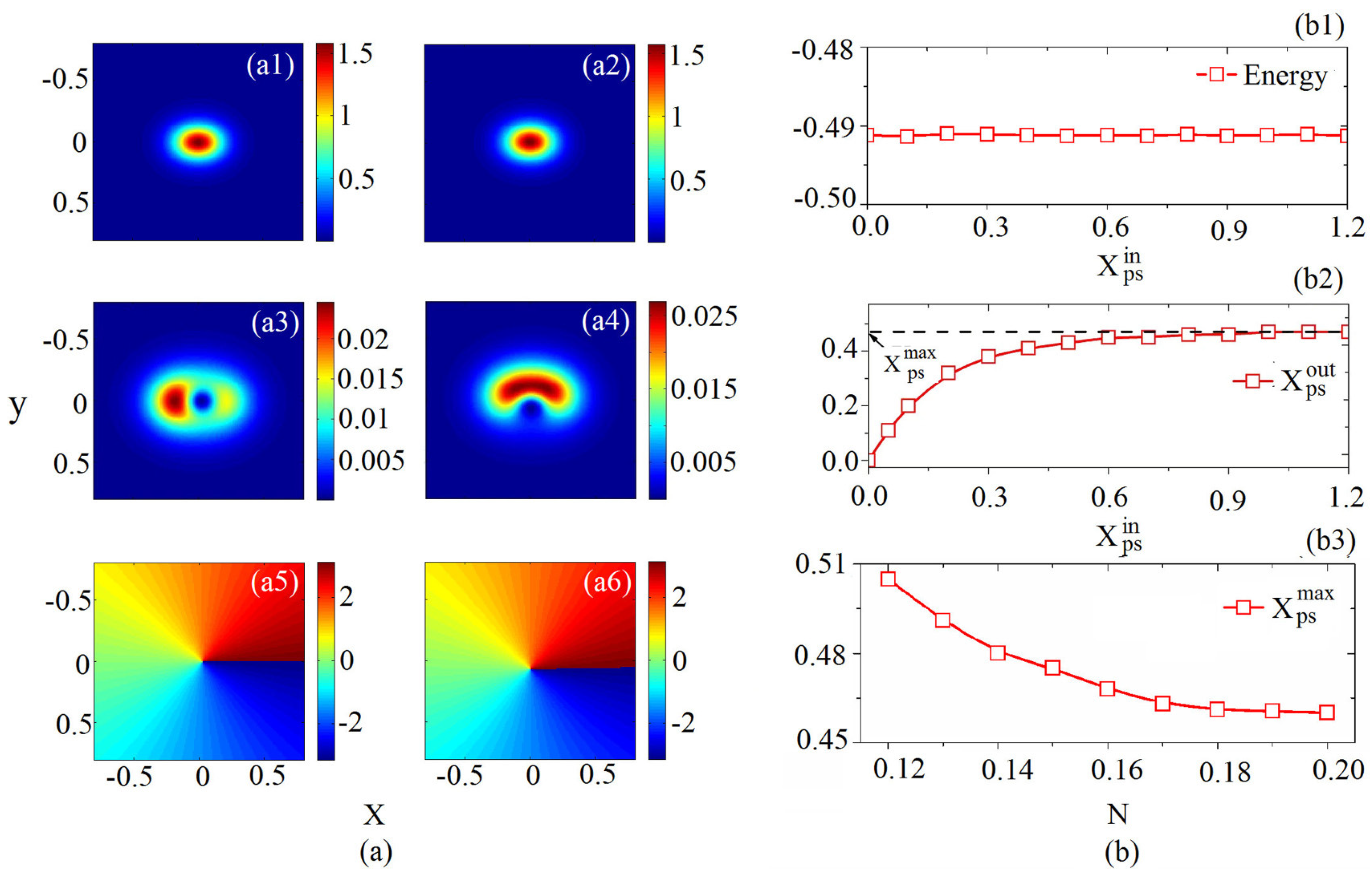
3. Semi-Vortices in Spinor SOC BEC with Pure DDI

In Equation (1), if $\Omega ,g,\gamma$ is set to be zero and $\beta$ is chosen to be $>0$ (Setting (i)), the system then corresponds to a spinor SOC BEC with pure DDI, and Equation (1) is reduced to:

$$\begin{array}{c}\hfill \begin{array}{c}\begin{array}{c}\hfill i{\partial }_t{\psi }_{+}=-\frac{1}{2}{\nabla }^2{\psi }_{+}+\lambda {\widehat{D}}^{[-]}{\psi }_{-}+\beta {\psi }_{+}\int d{\mathbf{r}}^{\prime }R(\mathbf{r}-{\mathbf{r}}^{\prime })(|{\psi }_{+}({\mathbf{r}}^{\prime }){|}^2+|{\psi }_{-}({\mathbf{r}}^{\prime }){|}^2),\end{array}\hfill \\ \begin{array}{c}\hfill i{\partial }_t{\psi }_{-}=-\frac{1}{2}{\nabla }^2{\psi }_{-}-\lambda {\widehat{D}}^{[+]}{\psi }_{+}+\beta {\psi }_{-}\int d{\mathbf{r}}^{\prime }R(\mathbf{r}-{\mathbf{r}}^{\prime })(|{\psi }_{+}({\mathbf{r}}^{\prime }){|}^2+|{\psi }_{-}({\mathbf{r}}^{\prime }){|}^2).\end{array}\hfill \end{array}\end{array}$$

(4)

The DDI kernel follows Equation (3) and ${cos}^2\theta \equiv {(x-x^{\prime })}^2/{|\mathbf{r}-{\mathbf{r}}^{\prime }|}^2$, which means the dipoles are all polarized in the 2D plane along the positive direction of the x axis. In order to obtain 2D solitons, the size of the soliton needs to be much larger than the cutoff $ϵ$, which requires proper setting of $ϵ$ and $\lambda$. In this section, $ϵ=0.05,\lambda =1$ is fixed [58].

The SOC term in Equation (4) breaks the Galilean invariance of the system, while the SOC and DDI terms both break the conservation of the angular momentum of the system. Thus, for spinor SOC BEC with pure DDI, the system is invariant with respect to specular reflections in the x-y plane:

$$\begin{array}{c}x\to -x,t\to -t,{\psi }_{\pm }\to \pm {\psi }_{\pm }^{\ast }\hfill \end{array}$$

(5)

$$\begin{array}{c}y\to -y,t\to -t,{\psi }_{\pm }\to {\psi }_{\pm }^{\ast }\hfill \end{array}$$

(6)

where * denotes the complex conjugate, which provides a combined symmetry of the system, which reads:

$$(x,y)\to (-x,-y),({\psi }_{+},{\psi }_{-})\to ({\psi }_{+},-{\psi }_{-})$$

(7)

The localized solution to Equation (4) is said to be symmetric if it keep this symmetry, otherwise it is said to be asymmetric [58]. Equation (4) can be numerically solved by the imaginary-time method [66,67].

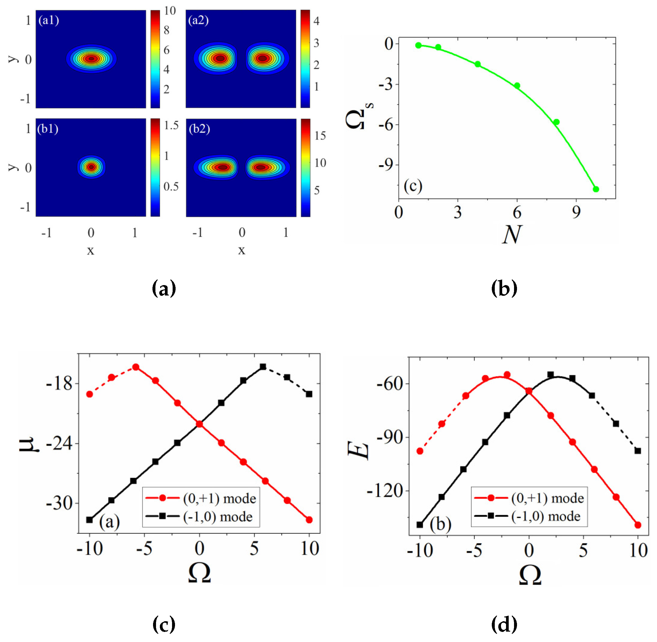
3.1. Symmetric Vortex Solitons

By using input trial wavefunction:

$${\varphi }_{+}^{(0)}=A_{1}exp(-{\alpha }_1{r}^2),{\varphi }_{-}^{(0)}=A_{2}r{e}^{i\theta }exp(-{\alpha }_2{r}^2),$$

(8)

stationary symmetric vortex solitons (SVS) can be obtained from Equation (4), and their stability can be checked via real-time evolution. Typical results of the stable SVS are shown in Figure 1.

As shown in Figure 1, all the semivortices (half vortices) have one component (${\varphi }_{+}$) carrying vorticity $S=0$ (called the fundamental component), and the other component (${\varphi }_{-}$) carries vorticity $S=+1$ (called the vortical component). What is more, all the stable SVs feature anisotropic patterns due to the anisotropic nature of the DDI, and at the same time, keep the symmetry in Equation (7). Traditionally, only anisotropic fundamental solitons are found to be stable in various settings, and no stable anisotropic vortex soliton is reported in literature. However, numerical analysis reveals that the anisotropic SVSs are stable if the total norm $N\equiv N_{+}+N_{-}=\int \int {|{\varphi }_{+}(x,y)|}^2$dr $+\int \int |{\varphi }_{-}{(x,y)|}^2$dr exceeds a threshold $N_{th}$ $\sim 0.12$. Under this threshold, both components of the SVS will become a breather mode showing oscillatory instability [58]. This instability is different from the system with contact attractive nonlinearity [49] where the nonlinearity itself will lead to the collapse of the soliton, and the long-range DDI will not cause the collapse, such that the stability of the SVS under DDI is easier to archive. Stable families of SVSs are found, and they fulfill the Vakhitov–Kolokolov (VK) criterion d$\mathsf{\mu }/$d$N<0$, which further sustain their stability.

3.2. Asymmetric Vortex Soliton

By using input trial wavefunction:

$${\varphi }_{+}^{(0)}=A_{1}exp(-{\alpha }_1{r}^2),{\varphi }_{-}^{(0)}=A_2|\mathbf{r}-{\mathbf{R}}_{ps}|exp(i{\theta }_{ps}-{\alpha }_2{r}^2).$$

(9)

the asymmetric vortex soliton can also be produced in this setting; where ${\mathbf{R}}_{ps}=X_{ps}^{in}\widehat{\mathbf{i}}+Y_{ps}^{in}\widehat{\mathbf{j}}$ is the initial offset of the vortex component with respect to the fundamental component and ${\theta }_{ps}$ is the angular coordinate for the vortex’s pivot placed at $\mathbf{r}={\mathbf{R}}_{ps}$. Typical results are shown in Figure 2.

The vortical component of these asymmetric vortex solitons (AVS) apparently breaks the symmetry of Equations (5) and (6), which is not seen in the settings with contact nonlinearity [49]. The AVS holds the same threshold $N\sim 0.12$ as the SVS, below which the AVS will convert to robust breather mode, as well. For any fixed value of $N>0.12$, there exists a continuous family of AVSs, parametrized by the offsets of the vortex’s pivot, $(X_{ps},Y_{ps})$. The energy of the AVSs in each family is highly degenerated, depending only on N (see Figure 2(b1)). The pivot of the vortex component in both directions exhibits saturation behavior, and the max value of the pivot decreases with the total norm N (see Figure 2(b2,b3)) [58]. These interesting results may originate from the anisotropic nature of DDI and open new possibilities for creating stable vortex 2D solitons in experiments, but no simple and intuitive explanation has yet been found.

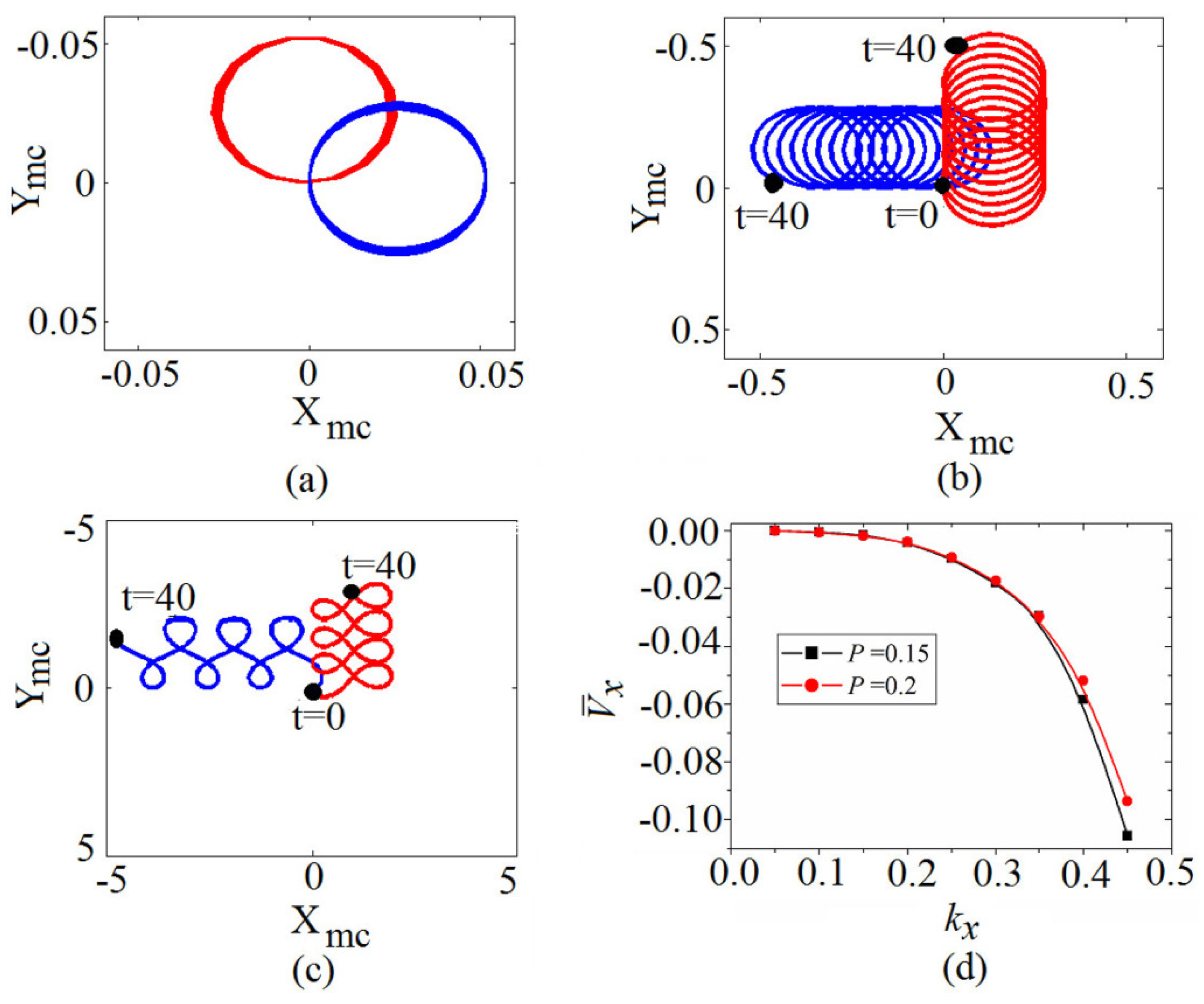
3.3. Mobility of the SVS and AVS

Although the SOC breaks the Galilean invariance of the system, analysis of the SVS and AVS reveals that they can be both kicked to move by applying a initial kick to the solution:

$${\psi }_{\pm }(\mathbf{r},t=0)={\varphi }_{\pm }exp(i\mathbf{k}·\mathbf{r})$$

(10)

By tracking the shape change and trajectory of the center of mass (c.m.) of the solitons (mainly determined by the fundamental component) via real-time evolution, three kinds of motion of the SVS can be identified, as shown in Figure 3.

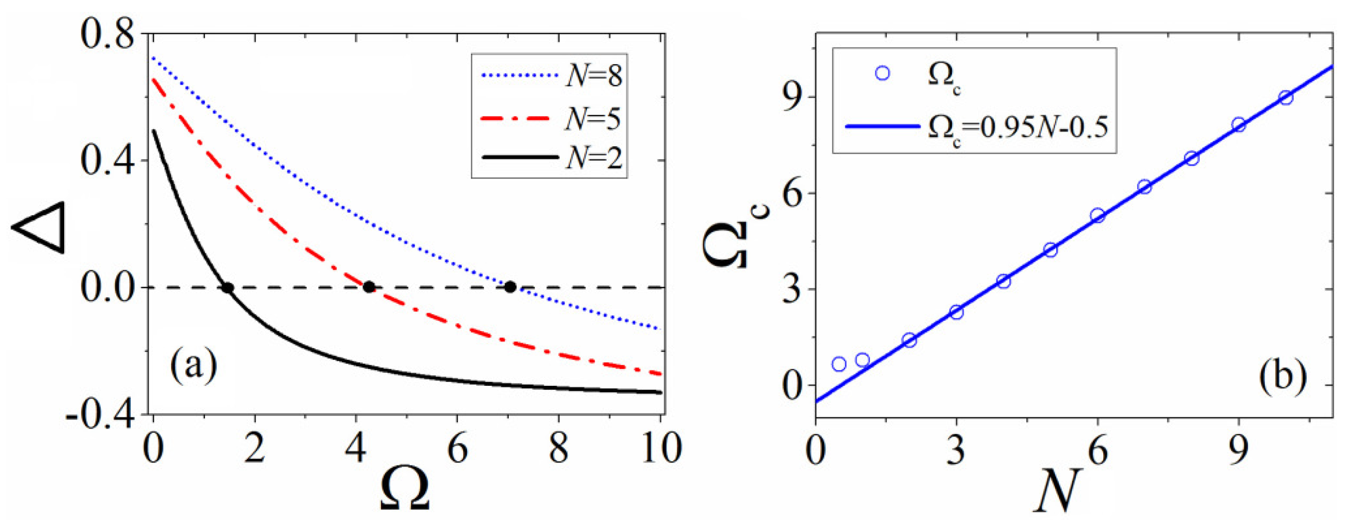
• For k smaller than a depinning threshold $k_d$, the SVS will be pinned to move in a circle trajectory (see Figure 3a) and is isotropic in both directions x and y.
• For $k>k_d$, the SVS is depinned and move with a negative effective mass (i.e., opposite the direction of the kick) in a spiral trajectory (see Figure 3b), but still isotropic in both directions.
• For $k>k_{upper}$ where $k_{upper}$ is another threshold larger than $k_d$, the SVS will undergo a more complex “lacy” trajectory and become anisotropic (see Figure 3c).

The AVS can also be kicked to move, but due to the anisotropy of the DDI and the asymmetric shape of the vortex component in that case, the motion pattern is far more complex than that of the SVS. The motion is highly anisotropic to the horizontal and vertical kick, and a kick in one direction will cause not only motion in this direction, but also in another direction. Under different kick parameters, the AVS can either exhibit pinning, spiral or ”lacy” motions, but no easy pattern, as SVS is yet to be clarified [58]. Typical examples of the motion of AVS are shown in Figure 4. These behaviors of mobility are important in the control and manipulation of solitons both in theory and experiments.

4. Semi-Vortices in Spinor SOC BEC with DDI and ZS

By adding a Zeeman splitting (ZS) term into Equation (4), the system now changes to spinor SOC BEC with DDI and ZS (Setting (ii)), with ZS strength $\Omega$, the sign of which can be altered between positive and negative. Using the same trial input Equation (9) and the same numerical methods, stable SVS similar to that in Figure 1 can also be produced in this setting [59] (However, in [59], AVS is used to describe the soliton to emphasize that they are the anisotropic vortex soliton. Actually, they are the SVS we discussed in the previous section with no pivot of the vortex component. To avoid conflict, we stick to using SVS here.). Typical results of the SVSs are displayed in Figure 5.

4.1. Shape Control of the SVS by ZS

It is found that the strength of the ZS can change the shape of the SVS. As shown in Figure 5, when the strength of ZS $\Omega =0$, the system goes back to Equation (4), and similar SVS are produced (Panels (a1), (a2)). Just like the SVS in Figure 1, the anisotropic nature of DDI deforms the fundamental and vortex component in the horizontal direction (longitudinal directions compared to the dipole orientation), creating two density maxima separated in this direction. For this reason, these SVSs are called horizontal SVS [59]. When $\Omega$ increases and exceeds a certain critical value ${\Omega }_c$, the shape of the SVS changes, especially for the vortex component (Panels (b1), (b2)), which now has two density maxima along the vertical directions (transverse directions compared to the dipole orientation; compare Panels (b2) and (a2)); therefore, it is called the vertical SVS. This change of shape is continuous with $\Omega$ increasing from zero, so at $\Omega ={\Omega }_c$, the SVS features an elliptic ring with no density maxima for any specific direction (Panel c2). The value of ${\Omega }_c$ can be determined numerically by defining a shape parameter:

$$\Delta =\frac{|{\varphi }_{-}^{max}{(x,0)|}^2-{|{\varphi }_{-}^{max}(0,y)|}^2}{|{\varphi }_{-}^{max}{(x,0)|}^2+{|{\varphi }_{-}^{max}(0,y)|}^2}$$

(11)

and the results are displayed in Figure 6.

Figure 6 shows clearly that the strength of ZS, $\Omega$, can be used as a shape control parameter to transform the SVS between horizontal and vertical mode. The critical value of this transition ${\Omega }_c$ has an almost linear relation with the total norm N, which can be explained qualitatively by noticing that at large $\Omega$ and a large N limit, the energy of DDI and ZS scales as $N^2$ and $\Omega N$, respectively [59]. Since this transition is the result of competition between DDI and ZS, the transition then must occur at $\Omega =const.\times N$, as indicated in Panel (b) of Figure 6.

4.2. Inverted SVS with $\Omega <0$

The SVSs discussed before this subsection all have $\Omega >0$, with their fundamental (with vorticity $S=0$) and vortical component (with vorticity $S=1$) taking the lower and higher energy position, respectively, which can be regarded as the ground state of the system. If $\Omega$ is switched to $<0$, then the fundamental and vortex component will switch their energy position, to be in the higher and lower energy state, respectively. This inverted state can be considered as the excited state of the system [59]. Such inverted SVS is confirmed to exist and be stable via methods used in the previous sections, setting $\Omega <0$. Typical results are displayed in Figure 7.

Families of stable inverted SVS can be identified through numerical results, which are all horizontal type (compare Figure 7 with Figure 1 and Figure 5), and no vertical type inverted SVS is found to exist. Despite all be excited states of the system, as indicated in Figure 7c,d, they surprisingly occupy a vast stable region, given $\Omega >{\Omega }_s$. Below, this $\Omega s$ inverted SVS still exists, but suffers spontaneous fragmentation instability (Panel (b)) [59]. Previously, only unstable excited states of SVS were found [49,68], and no stable excited SVS has been reported in the literature, especially stable SVS with a dominant vortex component. These findings provide new possibilities to create and manipulate 2D excited vortex solitons experimentally.

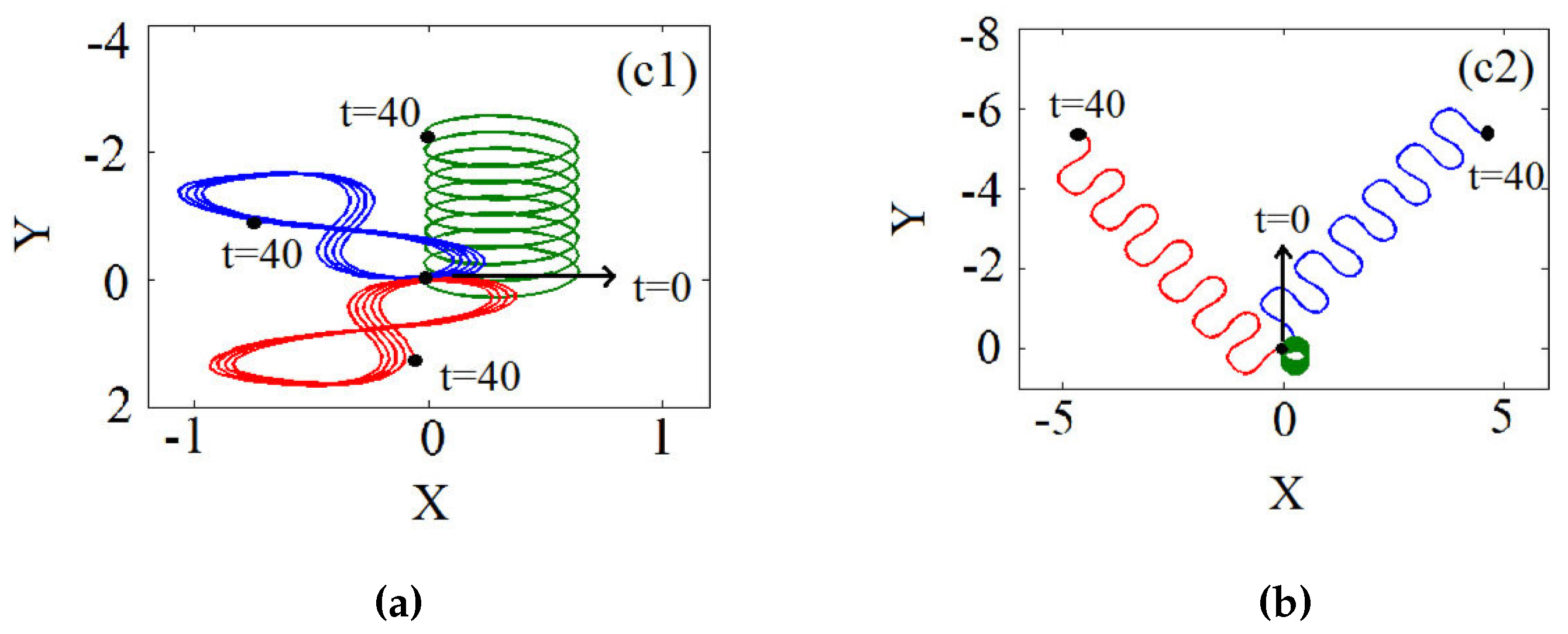
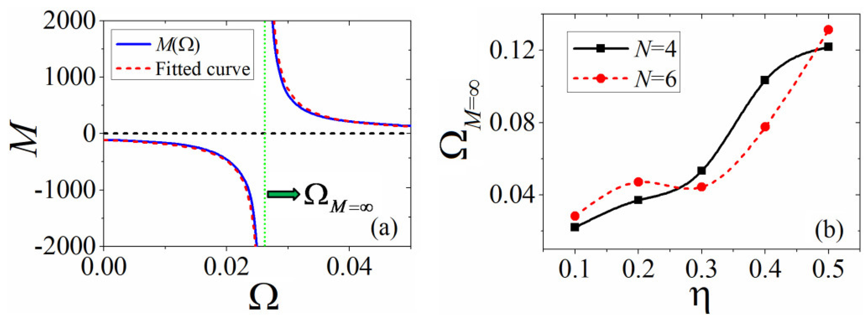
4.3. Mobility and Effective Mass Controlled by ZS

Besides controlling the shape of the SVS, enabling transitions between the horizontal and vertical type, Zeeman splitting also exhibits crucial effects on the mobility of the SVS. By defining the effective mass $M_{x,y}=P_{x,y}/V_{x,y}$ where:

$$\mathbf{P}=i\int d\mathbf{r}[(\Delta {\psi }_{+}^{\ast }){\psi }_{+}+(\Delta {\psi }_{-}^{\ast }){\psi }_{-}]$$

(12)

and $V_{x,y}$ is the velocity of the SVS, the motion of the SVS can be studied quantitatively. Numerical results show that as in Section 3.3, the SVS can be kicked to move and undergoes different types of motion depending on the kick strength. The effective mass defined above only applies to the spiral motion (see Figure 3b), and it is found that for spiral motion, changing $\Omega$ can switch the effective mass between positive and negative, via infinite divergence at a specific value $\Omega ={\Omega }_{M=\infty }$. Typical results are displayed in Figure 8. General conclusions can be drawn from these results:

• For $\Omega <{\Omega }_{M=\infty }$, the SVS possesses a negative effective mass, and it will move in the opposite directions of the kick. This is in accordance with results in Section 3.3, where $\Omega =0$.
• For $\Omega ={\Omega }_{M=\infty }$, the effective mass of SVS diverges to infinity, and the soliton will be pinned to move in a circular trajectory, similar to the motion shown in Panel (a) of Figure 3, which can be regarded as the immobility of the soliton.
• For $\Omega >{\Omega }_{M=\infty }$, the SVS possesses a positive effective mass, and it will move along the directions of the kick.
• For $\Omega \to \infty$, the effective mass approaches the total norm $M\to N$, since it becomes a usual single-component soliton.

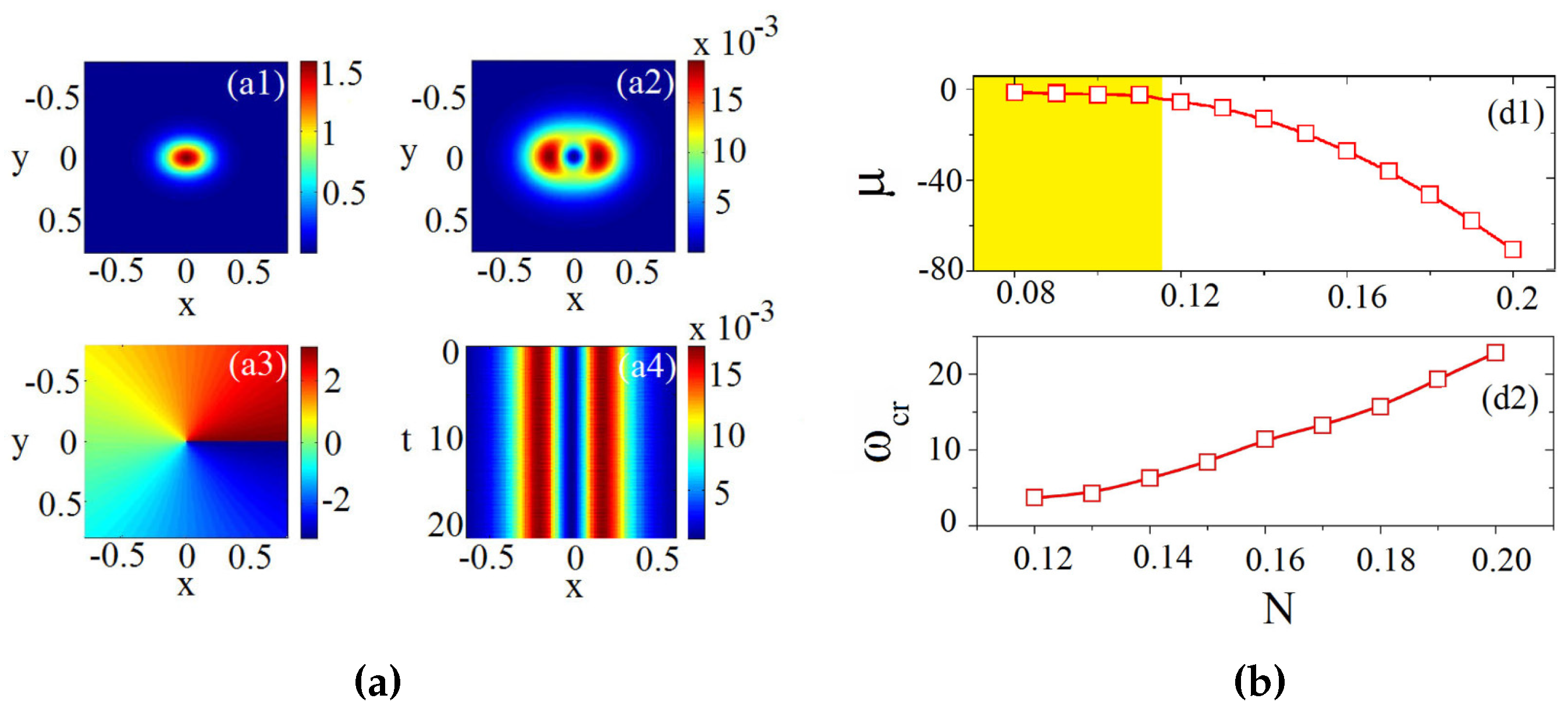
5. Gap Solitons in Spinor SOC BEC

Gap solitons (GS) are self-trapped modes existing in the spectral band gap of the system. The band gap generally is generated by certain types of spatially periodic potentials, such as Bragg gratings [69], wave guide arrays [21,70] and photonic crystals [17] in optics, or the optical lattice in BEC [23,24] and plasma medium [20,71]. Combined with SOC, 1D and 2D BEC gap solitons can also be produced in the optical lattice [43,44,72,73]. In these settings, the external potential, which creates the band structure, also exerts a spatial confinement on the solitons.

On the other hand, theoretical and numerical analysis reveals that by adding a Zeeman splitting, the SOC spinor BEC can support gap solitons in free space, with the collaboration of a DDI. Without spatial modulation, the energy gap is opened solely by the Zeeman splitting, which is a crucial ingredient to the SOC realization in experiments [74]. Families of stable isotropic and anisotropic gap solitons exist at the edge of the band gap, depending on the orientation of the dipolar BEC [60].

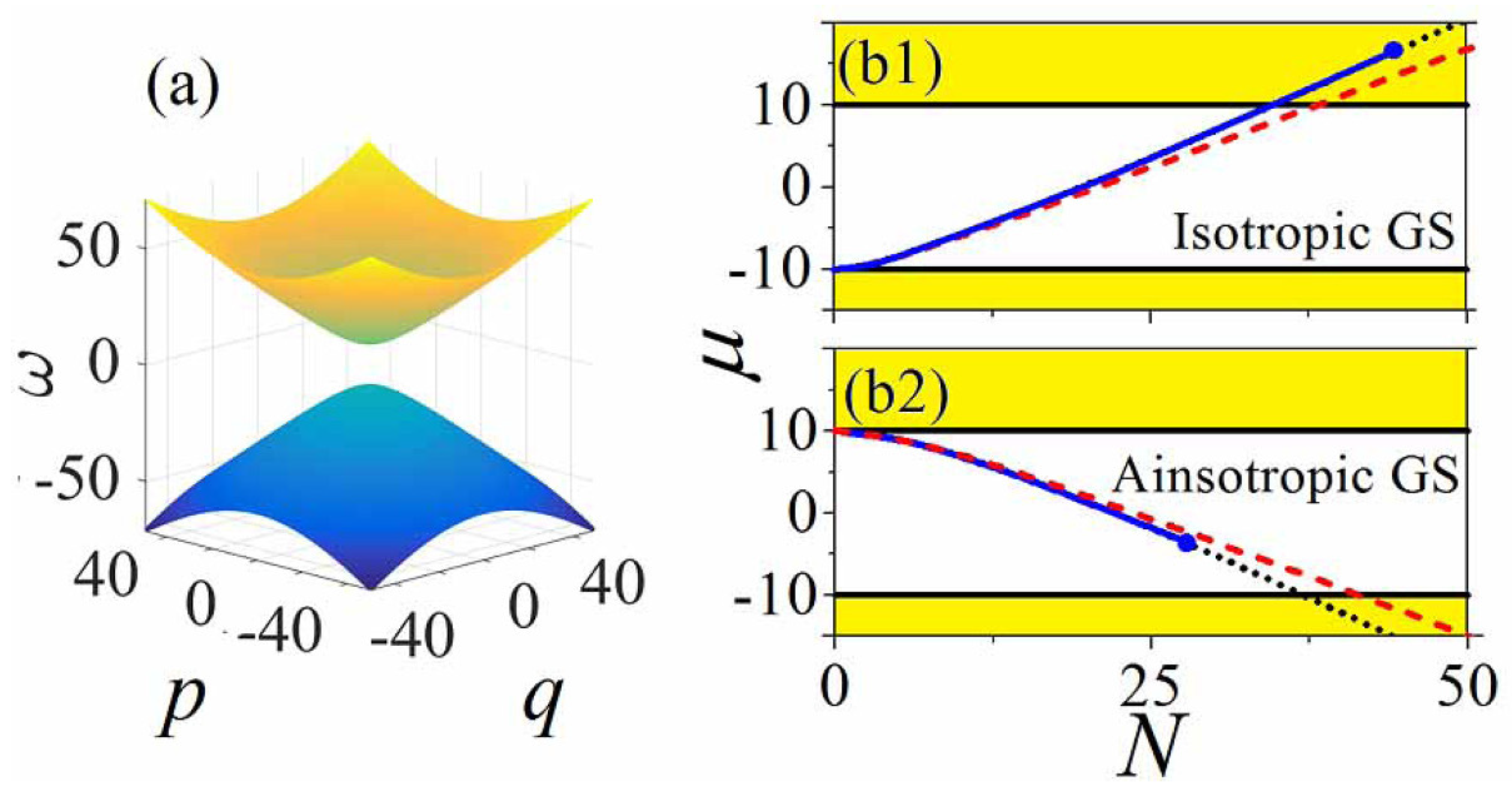
5.1. Isotropic and Anisotropic Families of the Gap Soliton

By setting $g=\gamma$ in Equation (1), the system now returns to a more general case with DDI, ZS and contact nonlinearity (Setting (iii)). Note that the sign of $\beta$ can be altered by rotating the magnetic field [75], and the sign of g can be switched through Feshbach resonance. This equation actually describes a 2D spinor BEC tightly trapped in the transverse (i.e., third) direction with a trapping size $a_{\perp }$, which requires the size of any soliton results to fulfill $l\gg a_{\perp }$. Meanwhile, the SOC strength needs to be strong enough to manifest effects experimentally, which requires $\beta \ge 1/a_{\perp }$. Together, these requirements give:

$$l\beta \gg 1$$

(13)

and Equation (1) shows the ratio of kinetic energy and the SOC term is $\sim 1/(l\beta )$, which implies under these settings that the kinetic term can be neglected safely. Equation (1) then reduces to:

$$\begin{array}{c}\hfill \begin{array}{c}\begin{array}{cc}\hfill i{\partial }_t{\psi }_{+}=\lambda {\widehat{D}}^{[-]}{\psi }_{-}-\Omega {\psi }_{+}& -(g|{\psi }_{+}{|}^2+g|{\psi }_{-}{|}^2){\psi }_{+}\hfill \\ & +\beta {\psi }_{+}\int d{\mathbf{r}}^{\prime }R(\mathbf{r}-{\mathbf{r}}^{\prime })(|{\psi }_{+}({\mathbf{r}}^{\prime }){|}^2+|{\psi }_{-}({\mathbf{r}}^{\prime }){|}^2),\hfill \end{array}\hfill \\ \begin{array}{cc}\hfill i{\partial }_t{\psi }_{-}=-\lambda {\widehat{D}}^{[+]}{\psi }_{+}+\Omega {\psi }_{-}& -(g|{\psi }_{+}{|}^2+g|{\psi }_{-}{|}^2){\psi }_{-}\hfill \\ & +\beta {\psi }_{-}\int d{\mathbf{r}}^{\prime }R(\mathbf{r}-{\mathbf{r}}^{\prime })(|{\psi }_{+}({\mathbf{r}}^{\prime }){|}^2+|{\psi }_{-}({\mathbf{r}}^{\prime }){|}^2).\hfill \end{array}\hfill \end{array}\end{array}$$

(14)

Linearization to Equation (14) with ${\psi }_{\pm }\sim exp(ipx+iqy-iwt)$ leads to the dispersion relation:

$${\omega }^2={\Omega }^2+{\beta }^2(p^2+q^2)$$

(15)

which opens a band gap of width $2\Omega$ in free space, as shown in Figure 9, where $p,q$ are the quasi-momentum of the soliton in the $x,y$ direction, respectively. Note that this energy gap will close if the kinetic terms are included [60].

Analytic and numerical solutions to Equation (14) can be carried our [60], and the results show that without DDI ($\beta =0$), the equation gives no soliton solutions when the contact nonlinearity is attractive ($g<0$) and gives the unstable Townes’ solitons when contact nonlinearity is repulsive ($g>0$); thus, no stable solitons can be obtained under this setting without DDI. It needs to be noted that the above conclusions are drawn under conditions that the strengths of self- and cross- interactions are equal, $g=\gamma$ in Equation (1). Actually, the relative ratio between g and $\gamma$ can be adjusted by the Feshbach resonance technique experimentally, by applying a DC magnetic field to the spinor BEC [76,77,78], and very recent research revealed [79] that for unequal g and $\gamma$, even without DDI, a continuous family of stable gap solitons exists in the upper band provided that $\gamma /g$ is less than a certain critical value ($\gamma /g<0.77$ in [79]).

On the contrary, without contact nonlinearity ($g=0$), but with DDI present ($\beta >0$), the system can produce stable isotropic solitons near the bottom edge of the gap when the DDI takes the isotropic kernel (i.e., $\theta =0$ in Equation (3) where the dipoles are oriented perpendicular to the system’s plane) and stable anisotropic solitons near the top edge of the gap when the DDI takes the anisotropic kernel (i.e., $\theta \ne 0$ in Equation (3) where the dipoles are oriented parallel to the system’s plane), as shown in Figure 9. With increasing total norm N, the isotropic gap solitons will extend as a continuous stable family across the full band into the upper Bloch band to become an embedded soliton (ES) [80,81], and it will terminate its stability as an ES when N exceeds a certain critical value $N>N_{max}$ (see Figure 9(b1)). The anisotropic gap solitons will also extend to a continuous family with increasing N, but it always terminates stability in the band (see Figure 9(b2)). To compare with experimental settings, an estimate gives the number of atoms constituting the gap soliton ranging from $N\sim {10}^3$ to $N\sim {10}^4$, by using values of the magnetic moment of ${}^{52}$Cr or ${}^{164}$Dy atoms and the strength of transverse trapping potential ${\omega }_{\perp }\sim 100$ Hz, which is feasible by current experimental techniques [60].

5.2. Mobility of the Gap Soliton

Both isotropic and anisotropic gap solitons can be kicked to move. For isotropic GS, it effective mass is always negative, in accordance with the generic features of GS [20,71]. However, for anisotropic GS, its effective mass is positive. Typical results are shown in Figure 10. For both types of GS, the effective mass varies almost linearly with the total norm N, and at small N, the effective mass is isotropic along the x and y directions, but exhibits anisotropy with increasing of N.

5.3. Effects of Contact Nonlinearity

The conclusions in Section 5.1 are drawn without contact nonlinearity, i.e., for $g=0$ in Equation (14). The effects of contact nonlinearity can be investigated numerically. The system is found to have an intrinsic stable boundary $g_{cr}\simeq \pm 0.25$ for isotropic and anisotropic GS, respectively. Thus, the isotropic GSs are stable if $g<0.25$, and the anisotropic GSs are stable if $g>-0.25$ (recall that $g<0$ and $g>0$ correspond to repulsive contact linearity for isotropic GS and anisotropic GS, respectively), which means the GSs are completely stable when arbitrarily strong contact nonlinearity is repulsive. On the other hand, due to the critical collapse effect of the contact nonlinearity, the norm of isotropic and anisotropic solitons cannot exceed certain limits, which is determined by the norm of the Townes’ soliton $N_T\simeq 5.85$, resulting in an exist condition for isotropic and anisotropic GS:

$$\begin{array}{c}\hfill \begin{array}{ccc}{g}_{iso}\hfill & \hfill <& N_T/(\Omega N)\hfill \\ g_{aniso}\hfill & \hfill >& -N_T/(\Omega N)\hfill \end{array}\end{array}$$

(16)

Between these two limits, that is $0.25<g_{iso}<N_T/(\Omega N)$ and $-N_T/(\Omega N)<g_{aniso}<-0.25$, the GSs are unstable and spontaneously transform into breathers in propagation [60].

6. Conclusions

We discussed in this review several settings of creating stable vortex 2D solitons in free space. By SOC combined with attractive anisotropic DDI, the continuous family of symmetric (SVS) and asymmetric (AVS) vortex soliton can be produced in spinor BEC. By adding a Zeeman splitting (ZS), the shape of the SVS can be switched between the horizontal and vertical type, the effective mass of the SVS can be altered from positive to negative and cross a divergence point where the effective mass goes to infinity and the SVS can be effectively pinned to be immobile. Inverted SVS is found to exist stably with the sign of ZS altered, despite the fact that it is actually the excited state of the system, which is new to the understanding of excited vortex solitons. The ZS also generates a spectral band structure in the system, which supports the continuous family of gap solitons (GS) in free space. Extensions to these research works is interesting to consider, especially on how to embed these findings into 3D settings, where the collapse effects are far stronger than in 2D, and even with the help of long-range DDI, d-wave collapse can easily destroy the soliton. Recent studies point out that combining SOC, DDI with the Lee-Huang-Yang (LHY) correction effect can suppress the collapsing or expanding of atoms, creating a stable quantum droplet in 3D free space [82]. Thus, extending the research works in this review to 3D settings under LHY corrections is an intriguing topic to investigate.

References

1. Malomed, B.A.; Mihalache, D.; Wise, F.; Torner, L. Spatiotemporal optical solitons. J. Opt. B 2005, 7, R53. [Google Scholar] [CrossRef]
2. Desyatnikov, A.S.; Kivshar, Y.S.; Torner, L. Optical vortices and vortex solitons. Prog. Opt. 2005, 47, 291–391. [Google Scholar] [Green Version]
3. Kivshar, Y.S.; Agrawal, G.P. Optical Solitons: From Fibers to Photonic Crystals; Academic Press: San Diego, CA, USA, 2003. [Google Scholar]
4. Griffin, A.; Snoke, D.W.; Stringari, S. Bose-Einstein Condensation; Cambridge University Press: New York, NY, USA, 1995. [Google Scholar]
5. Bauer, D.M.; Lettner, M.; Vo, C.; Rempe, G.; Dürr, S. Control of a magnetic Feshbach resonance with laser light. Nat. Phys. 2009, 5, 339–342. [Google Scholar] [CrossRef] [Green Version]
6. Yan, M.; DeSalvo, B.J.; Ramachandhran, B.; Pu, H.; Killian, T.C. Controlling Condensate Collapse and Expansion with an Optical Feshbach Resonance. Phys. Rev. Lett. 2013, 110, 123201. [Google Scholar] [CrossRef] [PubMed]
7. Fibich, G.; Papanicolaou, G. Self-focusing in the perturbed and unperturbed nonlinear Schrödinger equation in critical dimension. SIAM J. Appl. Math. 1999, 60, 183–240. [Google Scholar] [CrossRef]
8. Bergé, L. Wave collapse in physics: principles and applications to light and plasma waves. Phys. Rep. 1998, 303, 259–370. [Google Scholar] [CrossRef]
9. Kuznetsov, E.A.; Dias, F. Bifurcations of solitons and their stability. Phys. Rep. 2011, 507, 43. [Google Scholar] [CrossRef]
10. Torruellas, W.E.; Wang, Z.; Hagan, D.J.; VanStryland, E.W.; Stegeman, G.I.; Torner, L.; Menyuk, C.R. Observation of Two-Dimensional Spatial Solitary Waves in a Quadratic Medium. Phys. Rev. Lett. 1995, 74, 5036. [Google Scholar] [CrossRef] [PubMed]
11. Liu, X.; Beckwitt, K.; Wise, F. Two-dimensional optical spatiotemporal solitons in quadratic media. Phys. Rev. E 2000, 62, 1328. [Google Scholar] [CrossRef]
12. Quiroga-Teixeiro, M.; Michinel, H. Stable azimuthal stationary state in quintic nonlinear optical media. J. Opt. Soc. Am. B 1997, 14, 2004–2009. [Google Scholar] [CrossRef]
13. Mihalache, D.; Mazilu, D.; Crasovan, L.-C.; Towers, I.; Buryak, A.V.; Malomed, B.A.; Torner, A.; Torres, J.P.; Lederer, F. Stable Spinning Optical Solitons in Three Dimensions. Phys. Rev. Lett. 2002, 88, 073902. [Google Scholar] [CrossRef] [PubMed]
14. Mihalache, D.; Mazilu, D.; Crasovan, L.-C.; Towers, I.; Malomed, B.A.; Buryak, A.V.; Torner, L.; Lederer, F. Stable three-dimensional spinning optical solitons supported by competing quadratic and cubic nonlinearities. Phys. Rev. E 2002, 66, 016613. [Google Scholar] [CrossRef] [PubMed]
15. Falcaõ-Filho, E.L.; de Araujo, C.B.; Boudebs, G.; Leblond, H.; Skarka, V. Robust Two-Dimensional Spatial Solitons in Liquid Carbon Disulfide. Phys. Rev. Lett. 2013, 110, 013901. [Google Scholar] [CrossRef] [PubMed]
16. Gao, X.; Zeng, J. Two-dimensional matter-wave solitons and vortices in competing cubic-quintic nonlinear lattices. Front. Phys. 2018, 13, 130501. [Google Scholar] [CrossRef]
17. Fleischer, J.W.; Segev, M.; Efremidis, N.K.; Christodoulides, D.N. Observation of two-dimensional discrete solitons in optically induced nonlinear photonic lattices. Nature 2003, 422, 147–150. [Google Scholar] [CrossRef] [PubMed]
18. Terhalle, B.; Richter, T.; Law, K.J.H.; Göries, D.; Rose, P.; Alexander, T.J.; Kevrekidis, P.G.; Desyatnikov, A.S.; Krolikowski, W.; Kaiser, F.; et al. Observation of double-charge discrete vortex solitons in hexagonal photonic lattices. Phys. Rev. A 2009, 79, 043821. [Google Scholar] [CrossRef] [Green Version]
19. Minardi, S.; Eilenberger, F.; Kartashov, Y.V.; Szameit, A.; Röpke, U.; Kobelke, J.; Schuster, K.; Bartelt, H.; Nolte, S.; Torner, L.; et al. Three-Dimensional Light Bullets in Arrays of Waveguides. Phys. Rev. Lett. 2010, 105, 263901. [Google Scholar] [CrossRef] [PubMed]
20. Cerda-Méndez, E.A.; Sarkar, D.; Krizhanovskii, D.N.; Gavrilov, S.S.; Biermann, K.; Skolnick, M.S.; Santos, P.V. Exciton-Polariton Gap Solitons in Two-Dimensional Lattices. Phys. Rev. Lett. 2013, 111, 146401. [Google Scholar] [CrossRef] [PubMed]
21. Garanovich, I.L.; Longhi, S.; Sukhorukov, A.A.; Kivshar, Y.S. Light propagation and localization in modulated photonic lattices and waveguides. Phys. Rep. 2012, 518, 1–79. [Google Scholar] [CrossRef]
22. Lederer, F.; Stegeman, G.I.; Christodoulides, D.N.; Assanto, G.; Segev, M.; Silberberg, Y. Discrete solitons in optics. Phys. Rep. 2008, 463, 1–126. [Google Scholar] [CrossRef]
23. Morsch, O.; Oberthaler, M. Dynamics of Bose-Einstein condensates in optical lattices. Rev. Mod. Phys. 2006, 78, 179–215. [Google Scholar] [CrossRef]
24. Eiermann, B.; Anker, T.; Albiez, M.; Taglieber, M.; Treutlein, P.; Marzlin, K.-P.; Oberthaler, M.K. Bright Bose-Einstein Gap Solitons of Atoms with Repulsive Interaction. Phys. Rev. Lett. 2004, 92, 230401. [Google Scholar] [CrossRef] [PubMed]
25. Peccianti, M.; Conti, C.; Assanto, G.; de Luca, A.; Umeton, C. Routing of anisotropic spatial solitons and modulational instability in liquid crystals. Nature 2004, 432, 733–737. [Google Scholar] [CrossRef] [PubMed]
26. Ghofraniha, N.; Conti, C.; Ruocco, G.; Trillo, S. Shocks in Nonlocal Media. Phys. Rev. Lett. 2007, 99, 043903. [Google Scholar] [CrossRef] [PubMed]
27. Armaroli, A.; Trillo, S.; Fratalocchi, A. Suppression of transverse instabilities of dark solitons and their dispersive shock waves. Phys. Rev. A 2009, 80, 053803. [Google Scholar] [CrossRef]
28. Maucher, F.; Henkel, N.; Saffman, M.; Królikowski, W.; Skupin, S.; Pohl, T. Rydberg-Induced Solitons: Three-Dimensional Self-Trapping of Matter Waves. Phys. Rev. Lett. 2011, 106, 170401. [Google Scholar] [CrossRef] [PubMed]
29. Raghunandan, M.; Mishra, C.; Lakomy, K.; Pedri, P.; Santos, L.; Nath, R. Two-dimensional bright solitons in dipolar Bose-Einstein condensates with tilted dipoles. Phys. Rev. A 2015, 92, 013637. [Google Scholar] [CrossRef]
30. Huang, J.S.; Jiang, X.D.; Chen, H.Y.; Fan, Z.W.; Pang, W.; Li, Y.Y. Quadrupolar matter-wave soliton in two-dimensional free space. Front. Phys. 2015, 10, 1–7. [Google Scholar] [CrossRef]
31. Li, Y.; Liu, J.; Pang, W.; Malomed, B.A. Matter-wave solitons supported by field-induced dipole-dipole repulsion with a spatially modulated strength. Phys. Rev. A 2013, 88, 053630. [Google Scholar] [CrossRef]
32. Li, Y.-Y.; Fan, Z.-W.; Luo, Z.-H.; Liu, Y.; He, H.-X.; Lv, J.-T.; Xie, J.-N.; Huang, C.-Q.; Tan, H.-S. Cross-symmetry breaking of two-component discrete dipolar matter-wave solitons. Front. Phys. 2017, 12, 124206. [Google Scholar] [CrossRef]
33. Li, Y.; Pang, W.; Xu, J.; Lee, C.; Malomed, B.A.; Santos, L. Long-range transverse Ising model built with dipolar condensates in two-well arrays. New J. Phys. 2017, 19, 013030. [Google Scholar] [CrossRef] [Green Version]
34. Li, Y.; Liu, J.; Pang, W.; Malomed, B.A. Lattice soliton with quadrupolar intersite interaction. Phys. Rev. A 2013, 88, 063635. [Google Scholar] [CrossRef]
35. Chen, G.; Liu, Y.; Huang, H. Mixed-mode solitons in quadrupolar BECs with spin-orbit coupling. Commun. Nonlinear Sci. Numer. Simul. 2017, 48, 318–325. [Google Scholar] [CrossRef]
36. Zhong, R.; Huang, N.; Li, H.; He, H.; Lü, J.; Huang, C. Matter-wave solitons supported by quadrupole quadrupole interactions and anisotropic discrete lattices. Int. J. Mod. Phys. B 2018, 32, 1850107. [Google Scholar] [CrossRef]
37. Xu, Y.; Zhang, Y.; Wu, B. Bright solitons in spin-orbit-coupled Bose-Einstein condensates. Phys. Rev. A 2013, 87, 013614. [Google Scholar] [CrossRef]
38. Xu, Y.; Zhang, Y.; Zhang, C. Bright solitons in a two-dimensional spin-orbit-coupled dipolar Bose-Einstein condensate. Phys. Rev. A 2015, 92, 013633. [Google Scholar] [CrossRef]
39. Xu, X.-Q.; Han, J.H. Spin-Orbit Coupled Bose-Einstein Condensate Under Rotation. Phys. Rev. Lett. 2011, 107, 200401. [Google Scholar] [CrossRef] [PubMed]
40. Sinha, S.; Nath, R.; Santos, L. Trapped Two-Dimensional Condensates with Synthetic Spin-Orbit Coupling. Phys. Rev. Lett. 2011, 107, 270401. [Google Scholar] [CrossRef] [PubMed]
41. Zhou, X.-F.; Zhou, J.; Wu, C.J. Vortex structures of rotating spin-orbit-coupled Bose-Einstein condensates. Phys. Rev. A 2011, 84, 063624. [Google Scholar] [CrossRef]
42. Sakaguchi, H.; Li, B. Vortex lattice solutions to the Gross-Pitaevskii equation with spin-orbit coupling in optical lattices. Phys. Rev. A 2013, 87, 015602. [Google Scholar] [CrossRef] [Green Version]
43. Kartashov, Y.V.; Konotop, V.V.; Abdullaev, F.K. Gap Solitons in a Spin-Orbit-Coupled Bose-Einstein Condensate. Phys. Rev. Lett. 2013, 111, 060402. [Google Scholar] [CrossRef] [PubMed]
44. Lobanov, V.E.; Kartashov, Y.V.; Konotop, V.V. Fundamental, Multipole and Half-Vortex Gap Solitons in Spin-Orbit Coupled Bose-Einstein Condensates. Phys. Rev. Lett. 2014, 112, 180403. [Google Scholar] [CrossRef] [PubMed]
45. Beličev, P.; Gligorić, G.; Petrović, J.; Maluckov, A.; Hadzievski, L.; Malomed, B.A. Composite localized modes in discretized spin-orbit-coupled Bose-Einstein condensates. J. Phys. B 2015, 48, 065301. [Google Scholar] [CrossRef]
46. Zhang, Y.P.; Xu, Y.; Busch, T. Gap solitons in spin-orbit-coupled Bose-Einstein condensates in optical lattices. Phys. Rev. A 2015, 91, 043629. [Google Scholar] [CrossRef]
47. Achilleos, V.; Frantzeskakis, D.J.; Kevrekidis, P.G.; Pelinovsky, D.E. Matter-Wave Bright Solitons in Spin-Orbit Coupled Bose-Einstein Condensates. Phys. Rev. Lett. 2013, 110, 264101. [Google Scholar] [CrossRef] [PubMed]
48. Salasnich, L.; Malomed, B.A. Localized modes in dense repulsive and attractive Bose-Einstein condensates with spin-orbit and Rabi couplings. Phys. Rev. A 2013, 87, 063625. [Google Scholar] [CrossRef] [Green Version]
49. Sakaguchi, H.; Li, B.; Malomed, B.A. Creation of two-dimensional composite solitons in spin-orbit-coupled self- attractive Bose-Einstein condensates in free space. Phys. Rev. E 2014, 89, 032920. [Google Scholar] [CrossRef] [PubMed]
50. Sakaguchi, H.; Malomed, B.A. Discrete and continuum composite solitons in Bose-Einstein condensates with the Rashba spin-orbit coupling in one and two dimensions. Phys. Rev. E 2014, 90, 062922. [Google Scholar] [CrossRef] [PubMed]
51. Salasnich, L.; Cardoso, W.B.; Malomed, B.A. Localized modes in quasi-two-dimensional Bose-Einstein condensates with spin-orbit and Rabi couplings. Phys. Rev. A 2014, 90, 033629. [Google Scholar] [CrossRef] [Green Version]
52. Malomed, B.A. Creating solitons by means of spin-orbit coupling. Europhys. Lett. 2018, 122, 36001. [Google Scholar] [CrossRef]
53. Liu, S.; Liao, B.; Kong, J.; Chen, P.; Lü, J.; Li, Y.; Huang, C.; Li, Y. Anisotropic Semi Vortices in Spinor Dipolar Bose Einstein Condensates Induced by Mixture of Rashba Dresselhaus Coupling. J. Phys. Soc. Jpn. 2018, 87, 094005. [Google Scholar] [CrossRef]
54. Kartashov, Y.M.; Malomed, B.A.; Konotop, V.V.; Lobanov, V.E.; Torner, L. Stabilization of solitons in bulk Kerr media by dispersive coupling. Opt. Lett. 2015, 40, 1045–1048. [Google Scholar] [CrossRef] [PubMed]
55. Huang, H.; Lyu, L.; Xie, M.; Luo, W.; Chen, Z.; Luo, Z.; Huang, C.; Fu, S.; Li, Y. Spatiotemporal solitary modes in a twisted cylinder waveguide shell with the self-focusing Kerr nonlinearity. Commun. Nonlinear Sci. Numer. Simulat. 2019, 67, 617–626. [Google Scholar] [CrossRef]
56. Zhong, R.; Chen, Z.; Huang, C.; Luo, Z.; Tan, H.; Malomed, B.A.; Li, Y. Self-trapping under the two-dimensional spin-orbit-coupling and spatially growingrepulsive nonlinearity. Front. Phys. 2018, 13, 130311. [Google Scholar] [CrossRef]
57. Huang, C.; Ye, Y.; Liu, S.; He, H.; Pang, W.; Malomed, B.A.; Li, Y. Excited states of two-dimensional solitons supported by spin-orbit coupling and field-induced dipole-dipole repulsion. Phys. Rev. A 2018, 97, 013636. [Google Scholar] [CrossRef] [Green Version]
58. Jiang, X.; Fan, Z.; Chen, Z.; Pang, W.; Li, Y.; Malomed, B.A. Two-dimensional solitons in dipolar Bose-Einstein Condensates with spin-orbit coupling. Phy. Rev. A 2016, 93, 023633. [Google Scholar] [CrossRef]
59. Liao, B.; Li, S.; Huang, C.; Luo, Z.; Pang, W.; Tan, H.; Malomed, B.A.; Li, Y. Anisotropic semivortices in dipolar spinor condensates controlled by Zeeman splitting. Phy. Rev. A 2017, 96, 043613. [Google Scholar] [CrossRef] [Green Version]
60. Li, Y.; Liu, Y.; Fan, Z.; Pang, W.; Fu, S.; Malomed, B.A. Two-dimensional dipolar gap solitons in free space with spin-orbit coupling. Phy. Rev. A 2017, 95, 063613. [Google Scholar] [CrossRef] [Green Version]
61. Lin, Y.J.; Jiménez-García, K.; Spielman, I.B. Spin-orbit-coupled Bose-Einstein condensates. Nature 2011, 471, 83–86. [Google Scholar] [CrossRef] [PubMed]
62. Deng, Y.; Cheng, J.; Jing, H.; Sun, C.-P.; Yi, S. Spin-Orbit-Coupled Dipolar Bose-Einstein Condensates. Phys. Rev. Lett. 2012, 108, 125301. [Google Scholar] [CrossRef] [PubMed] [Green Version]
63. Wu, Z.; Zhang, L.; Sun, W.; Xu, X.; Wang, B.; Ji, S.; Deng, Y.; Chen, S.; Liu, X.; Pan, J. Realization of two-dimensional spin-orbit coupling for Bose-Einstein condensates. Science 2016, 354, 83–88. [Google Scholar] [CrossRef] [PubMed] [Green Version]
64. Sinha, S.; Santos, L. Cold Dipolar Gases in Quasi-One- Dimensional Geometries. Phys. Rev. Lett. 2007, 99, 140406. [Google Scholar] [CrossRef] [PubMed]
65. Cuevas, J.; Malomed, B.A.; Kevrekidis, P.G.; Frantzeskakis, D.J. Solitons in quasi-one-dimensional Bose-Einstein condensates with competing dipolar and local interactions. Phys. Rev. A 2009, 79, 053608. [Google Scholar] [CrossRef] [Green Version]
66. Chiofalo, L.M.; Succi, S.; Tosi, P.M. Ground state of trapped interacting Bose-Einstein condensates by an explicit imaginary-time algorithm. Phys. Rev. E 2000, 62, 7438–7444. [Google Scholar] [CrossRef]
67. Yang, J.; Lakoba, T.I. Accelerated imaginary-time evolution methods for the computation of solitary waves. Stud. Appl. Math. 2008, 120, 265–292. [Google Scholar] [CrossRef]
68. Li, Y.; Luo, Z.; Liu, Y.; Chen, Z.; Huang, C.; Fu, S.; Tan, H.; Malomed, B.A. Two-dimensional solitons and quantum droplets supported by competing self- and cross-interactions in spin- orbit-coupled condensates. New J. Phys. 2017, 19, 113043. [Google Scholar] [CrossRef]
69. Eggleton, B.J.; Slusher, R.E.; de Sterke, C.M.; Krug, P.A.; Sipe, J.E. Bragg Grating Solitons. Phys. Rev. Lett. 1996, 76, 1627. [Google Scholar] [CrossRef] [PubMed]
70. Mandelik, D.; Morandotti, R.; Aitchison, J.S.; Silberberg, Y. Gap Solitons in Waveguide Arrays. Phys. Rev. Lett. 2004, 92, 093904. [Google Scholar] [CrossRef] [PubMed]
71. Ostrovskaya, E.A.; Abdullaev, J.; Fraser, M.D.; Desyatnikov, A.S.; Kivshar, Y.S. Self-Localization of Polariton Condensates in Periodic Potentials. Phys. Rev. Lett. 2013, 110, 170407. [Google Scholar] [CrossRef] [PubMed]
72. Kartashov, Y.V.; Konotop, V.V. Solitons in Bose-Einstein Condensates with Helicoidal Spin-Orbit Coupling. Phys. Rev. Lett. 2017, 118, 190401. [Google Scholar] [CrossRef] [PubMed]
73. Zhu, X.; Li, H.; Shi, Z. Defect matter-wave gap solitons in spin-orbit-coupled Bose-Einstein condensates in Zeeman lattices. Phys. Lett. A 2016, 380, 3253–3257. [Google Scholar] [CrossRef]
74. Campbell, D.L.; Juzeliūnas, G.; Spielman, I.B. Realistic Rashba and Dresselhaus spin-orbit coupling for neutral atoms. Phys. Rev. A 2011, 84, 025602. [Google Scholar] [CrossRef]
75. Giovanazzi, S.; Görlitz, A.; Pfau, T. Tuning the Dipolar Interaction in Quantum Gases. Phys. Rev. Lett. 2002, 89, 130401. [Google Scholar] [CrossRef] [PubMed]
76. Papp, S.B.; Pino, J.M.; Wieman, C.E. Tunable Miscibility in a Dual-Species Bose-Einstein Condensate. Phys. Rev. Lett. 2008, 101, 040402. [Google Scholar] [CrossRef] [PubMed]
77. Zhang, P.; Naidon, P.; Ueda, M. Independent Control of Scattering Lengths in Multicomponent Quantum Gases. Phys. Rev. Lett. 2009, 103, 133202. [Google Scholar] [CrossRef] [PubMed]
78. Wang, F.; Li, X.; Xiong, D.; Wang, D. A double species 23Na and 87Rb Bose-Einstein condensate with tunable miscibility via an interspecies Feshbach resonance. J. Phys. B At. Mol. Opt. Phys. 2016, 49, 015302. [Google Scholar] [CrossRef]
79. Sakaguchi, H.; Malomed, B.A. One- and two-dimensional gap solitons in spin-orbit-coupled systems with Zeeman splitting. Phys. Rev. A 2018, 97, 013607. [Google Scholar] [CrossRef] [Green Version]
80. Yang, J.; Malomed, B.A.; Kaup, D.J. Embedded Solitons in Second-Harmonic-Generating Systems. Phys. Rev. Lett. 1999, 83, 1958–1961. [Google Scholar] [CrossRef]
81. Yang, J. Fully localized two-dimensional embedded solitons. Phys. Rev. A 2010, 82, 053828. [Google Scholar] [CrossRef]
82. Schmitt, M.; Wenzel, M.; Böttcher, F.; Ferrier-barbut, I.; Pfau, T. Self-bound droplets of a dilute magnetic quantum liquid. Nature 2016, 539, 259–262. [Google Scholar] [CrossRef] [PubMed] [Green Version]
Figure 1. Stable symmetric vortex solitons (SVS) numerically obtained from Equation (4). (a) Stable SVS with total norm N = 0 . 15 . (a1,a2) present the density distribution of the fundamental and vortical component, | ϕ + ( x , y ) | 2 and | ϕ ( x , y ) | 2 , respectively. (a3) is the phase structure of the vortical component. (a4) is the direct run of this SVS. (b) The chemical potential μ versus N. The yellow area indicates where the SVS is subjected to oscillatory instability and transforms into breather mode [58].
Applsci 08 01771 g001
Figure 2. Stable asymmetric vortex solitons (AVS) numerically obtained from Equation (4). (a) Stable AVS with total norm N = 0 . 15 . The first column presents the density distribution of the fundamental and vortical component, | ϕ + ) | 2 and | ϕ | 2 , and the phase structure of ϕ , with ( X p s , Y p s ) = ( 0 . 04 , 0 ) . The second column is the AVS with ( X p s , Y p s ) = ( 0 , 0 . 065 ) . (b) Various relations between the input and output X p s with energy and the total norm of the AVS [58].
Applsci 08 01771 g002
Figure 3. Motion of the c.m. of kicked symmetric vortex solitons (SVS) with N = 0 . 15 . (a) The kick k = ( k x , k y ) = ( 0 . 05 , 0 ) (blue) and ( 0 , 0 . 05 ) (red), pinning in a circle. (b) k = ( 0 . 25 , 0 ) (blue) and ( 0 , 0 . 25 ) (red), spiral motion. (c) k = ( 0 . 5 , 0 ) (blue) and ( 0 , 0 . 5 ) (red), “lacy” motion. (d) Mean velocity of the spiral motion for N = 0 . 15 and 0 . 2 [58].
Applsci 08 01771 g003
Figure 4. Motion of the c.m. of kicked asymmetric vortex solitons (AVS) with N = 0 . 15 . (a) AVS with ( X p s , Y p s ) = ( 0 . 12 , 0 ) . The kick k = ( k x , k y ) = ( + 0 . 5 , 0 ) (blue curve), ( 0 . 5 , 0 ) (red curve) and ( 0 , + 0 . 5 ) (green curve). (b) ( X p s , Y p s ) = ( 0 . 26 , 0 ) with the same kick [58].
Applsci 08 01771 g004
Figure 5. Symmetric vortex solitons (SVS) with N = 5 . (a) Fundamental (a1) and vortex (a2) component of SVS with Ω = 0 ; (b) with Ω = 10 ; (c) with Ω = 4 . 23 [59].
Applsci 08 01771 g005
Figure 6. Shape change of the SVS controlled by the Zeeman splitting Ω . (a) Shape parameter Δ versus Ω with different N; the dashed line determines Ω c . (b) (Almost) linear relationship between Ω c and N [59].
Applsci 08 01771 g006
Figure 7. Stable inverted SVS with Ω < 0 . (a) Density distribution of fundamental and vortex component of inverted SVS with ( Ω , N ) = ( 6 , 1 . 82 ) (first row) and ( Ω , N ) = ( 10 , 10 . 8 ) (second row); (b) stable threshold Ω s versus N; (c) chemical potentials of the SVS with vortices in ψ + and ψ components ( S + , S ) = ( 0 , + 1 ) and its flip counterpart ( S + , S ) = ( 1 , 0 ) vs. Ω ; (d) the same as in (c), except for total energy E vs. Ω [59].
Applsci 08 01771 g007
Figure 8. Effective mass M of the SVS in spiral motion controlled by the Zeeman splitting Ω . (a) M versus Ω with N = 5 and fixed kick k = 0 . 2 . Divergence occurs at Ω M = = 0 . 0262 . The dashed curve is the fitting 3 / ( Ω Ω M = ) . (b) Ω M = vs. the kick strength η with different N [59].
Applsci 08 01771 g008
Figure 9. Band gap and gap solitons of spin-orbit-coupling (SOC) spinor BEC with dipole-dipole interaction (DDI), Zeeman splitting (ZS) and contact nonlinearity. (a) The band gap structure described by Equation (15) with ( β , Ω ) = ( 1 , 10 ) . (b) Isotropic and anisotropic 2D gap solitons. The yellow area is the band; the white area is the gap. The blue curve is the branch of gap solitons found numerically, divided by the blue dot into stable (solid) and unstable (dashed) segments. The red dashed curve is the analytical prediction based on Equation (14) [60]. GS, gap solitons.
Applsci 08 01771 g009
Figure 10. Effective mass for isotropic (left) and anisotropic (right) 2D GS under kick in the x and y directions [60].
Applsci 08 01771 g010