Article

Multi-Robot Path Planning Method Using Reinforcement Learning

1
Department of Electrical Engineering Yeungnam University, Gyeongsan 38541, Korea
2
TycoAMP, Gyeongsan 38541, Korea
3
Korea Polytechnic VII, Changwon 51519, Korea
4
School of Control and Computer Engineering, North China Electric Power University, Beijing 102206, China
*
Author to whom correspondence should be addressed.
Appl. Sci. 2019, 9(15), 3057; https://doi.org/10.3390/app9153057
Submission received: 29 June 2019 / Revised: 21 July 2019 / Accepted: 26 July 2019 / Published: 29 July 2019
(This article belongs to the Special Issue Mobile Robots Navigation)

Abstract

:
This paper proposes a noble multi-robot path planning algorithm using Deep q learning combined with CNN (Convolution Neural Network) algorithm. In conventional path planning algorithms, robots need to search a comparatively wide area for navigation and move in a predesigned formation under a given environment. Each robot in the multi-robot system is inherently required to navigate independently with collaborating with other robots for efficient performance. In addition, the robot collaboration scheme is highly depends on the conditions of each robot, such as its position and velocity. However, the conventional method does not actively cope with variable situations since each robot has difficulty to recognize the moving robot around it as an obstacle or a cooperative robot. To compensate for these shortcomings, we apply Deep q learning to strengthen the learning algorithm combined with CNN algorithm, which is needed to analyze the situation efficiently. CNN analyzes the exact situation using image information on its environment and the robot navigates based on the situation analyzed through Deep q learning. The simulation results using the proposed algorithm shows the flexible and efficient movement of the robots comparing with conventional methods under various environments.

1. Introduction

Machine learning, which is one of the fields of artificial intelligence and is a technology to implement functions such as human learning ability by computer, has been studied in various concessions mainly used in the field of signal processing and image processing [1,2,3], such as speech recognition [4,5], natural language processing [6,7,8], and medical treatment [9,10]. Since the performance using machine learning shows good results, it will play an important role in the 4th industrial revolution as is well known in Alpha machine learning [11]. Reinforced learning is the training of machine learning models to make a sequence of decisions so that a robot learns to achieve a goal in an uncertain, potentially complex environment by selecting the action to be performed according to the environment without an accurate system model. When learning data is not provided, some actions are taken to compensate the system for learning. Reinforcement learning, which includes actor critic [12,13,14] structure and q learning [15,16,17,18,19,20,21], has many applications such as scheduling, chess, and robot control based on image processing, path planning [22,23,24,25,26,27,28,29] and etc. Most of the existing studies using reinforcement learning exclusively the performance in simulation or games. In multi-robot control, reinforcement learning and genetic algorithms have some drawbacks that have to be compensated for. In contrast to the control of multiple motors in a single robot arm, reinforcement learning of the multiple robots for solving one task or multiple tasks is relatively inactive.
This paper deals with information and strategy around reinforcement learning for multi-robot navigation algorithm [30,31,32,33] where each robot can be considered as a dynamic obstacle [34,35] or cooperative robot depending on the situation. That is, each robot in the system can perform independent actions and simultaneously collaborate with each other depending on the given mission. After the selected action, the relationship with the target is evaluated, and rewards or penalty is given to each robot to learn.
The robot learns the next action based on the learned data when it selects the next action, and after several learning, it moves to the closest target. By interacting with the environment, robots exhibit new and complex behaviors rather than existing behaviors. The existing analytical methods suffer from adaptation to complex and dynamic systems and environments. By using Deep q learning [36,37,38] and CNN [39,40,41], reinforcement learning is performed on the basis of image, and the same data as the actual multi-robot is used to compare it with the existing algorithms.
In the proposed algorithm, the global image information in the multi-robot provides the robots with higher autonomy comparing with conventional robots. In this paper, we propose a noble method for a robot to move quickly to the target point by using reinforcement learning for path planning of a multi-robot system. In this case, reinforcement learning is a Deep q learning that can be used in a real mobile robot environment by sharing q parameters for each robot. In various 2D environments such as static and dynamic environment, the proposed algorithm spends less searching time than other path planning algorithms.

2. Reinforcement Learning

Reinforcement learning is the training of machine learning models to make a sequence of decisions through trial and error in a dynamic environment. The robots learn to achieve a goal in an uncertain, potentially complex environment through programming the object by reward or penalty.
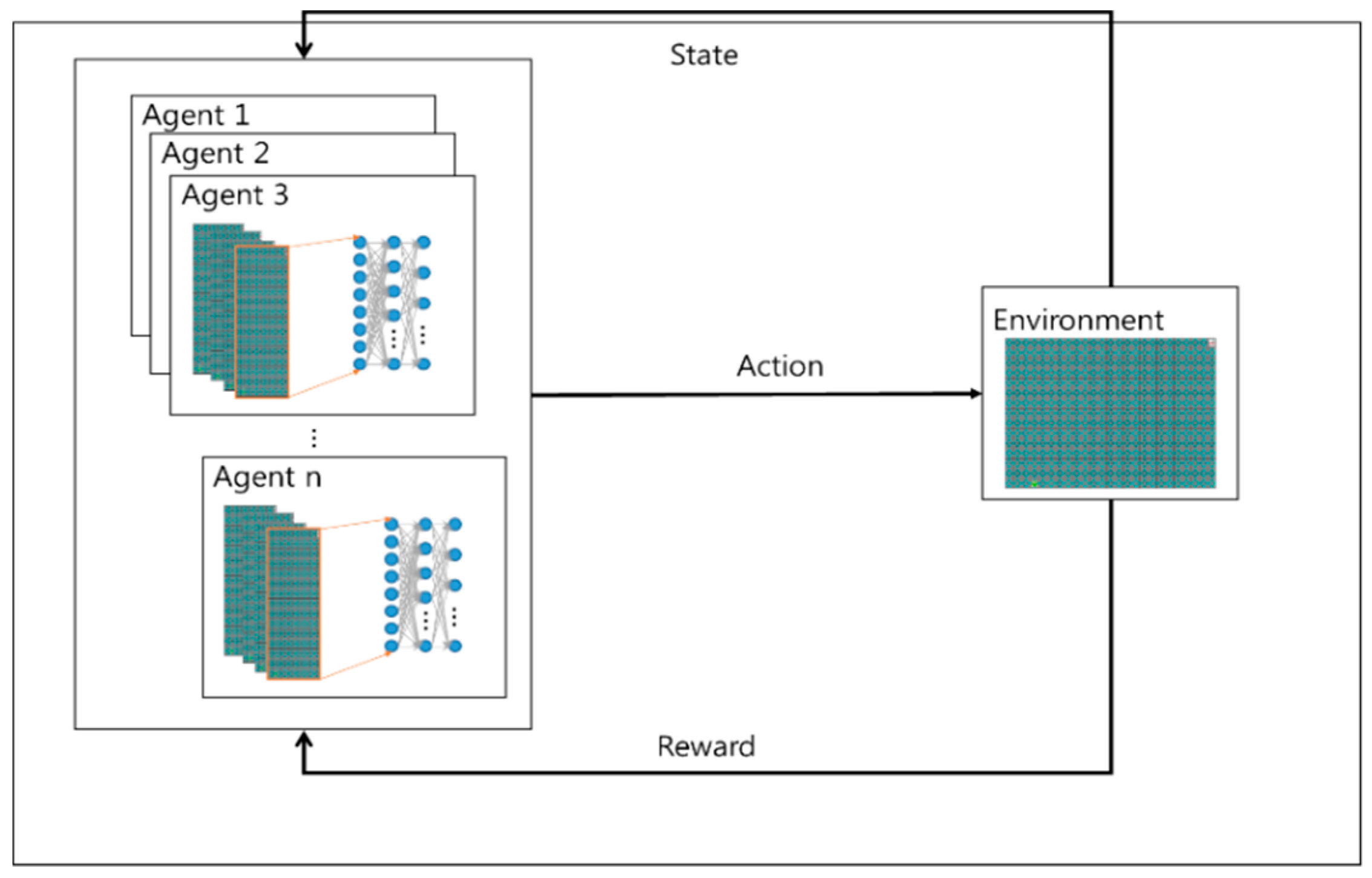
Figure 1 shows a general reinforcement learning, a robot which selects the action a as output recognizes the environment and receives the state, s, of the environment. The state of the behavior is changed, and the state transition is delivered to the individual as a reinforcement signal called a reinforcement signal. The behavior of the individual robot is selected in such a way as to increase the sum of the enhancement signal values over a long period of time.
One of the most distinguishable differences of reinforcement learning from supervised learning is that it does not use the representation of the link between input and output. After choosing an action, it is rewarded and knows the following situation. Another difference is that the online features of reinforcement learning are important since the computation of the system takes place at the same time as learning. One of the reinforcement learning features, Deep q learning, is characterized by the temporal difference method, which allows learning directly by experience and does not need to wait until the final result to calculate the value of each state like dynamic programming.
When a robot is moving in a discrete, restrictive environment, it chooses one of a set of definite behaviors at every time interval and assumes that it is in Markov state; the state changes to the probability s of different.
Pr[st+1] = s’[st, at] = Pr[at]
At every time interval t, a robot can get status s from the environment and then take action at. It receives a stochastic prize r, which depends on the state and behavior of the expected prize Rst to find the optimal policy that an entity wants to achieve.
R s t ( a i )   = E { i = 0 Y j r t + j }
The discount factor means that the rewards received at t time intervals are less affected than the rewards currently received. The operational value function Va is calculated using the policy function π and the policy value function Vp as shown in Equation (3). The state value function for the expected prize when starting from state s and following the policy is expressed by the following equation.
V a ( s t )     R s ( π ( s t ) ) + Y u P x y [ π ( s t ) ] V p ( s t )
It is proved that there is at least one optimal policy as follows. The goal of Q-learning is to set an optimal policy without initial conditions. For the policy, define the Q value as follows.
Q p ( s t , a t ) =   R s ( a t )   +   Y u P x y [ π ( s t ) ] V p ( y )
Q(st, at) is the newly calculated Q(st−1, at−1), and Q(st−1, at−1) corresponding to the next state by the current Q(st−1, at−1) value and the current Q(st−1, at−1).

3. Proposed Algorithm

Figure 2 is the form of the proposed. The proposed algorithm uses empirical representation technique. The learning experience that occurs at each time step through multiple episodes to be stored in the dataset is called memory regeneration. The learning data samples are used for updating with a certain probability in the reconstructed memory each time. Data efficiency can be improved by reusing experience data and reducing correlations between samples.
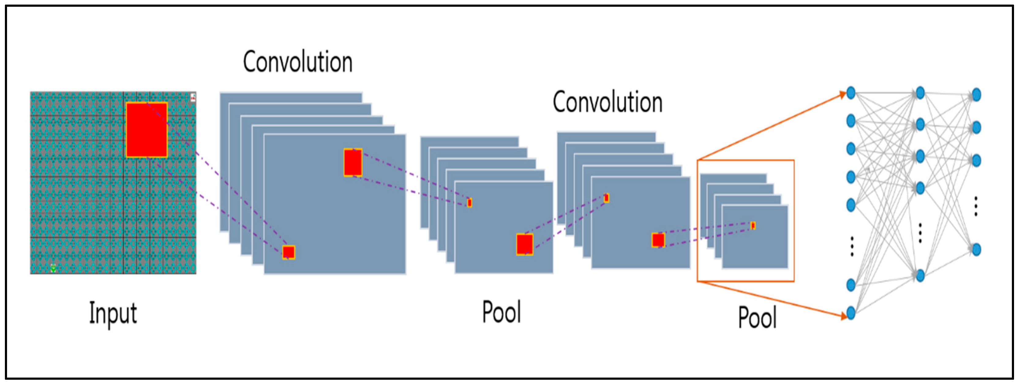
Without treating each pixel independently, we use the CNN algorithm to understand the information in the images. The transformation layer transmits the feature information of the image to the neural network by considering the area of the image and maintaining the relationship between the objects on the screen. CNN extracts only feature information from image information. The reconstructed memory to store the experience basically stores the agent’s experience and uses it randomly when learning neural networks. Through this process, which prevents learning about immediate behavior in the environment, the experience is sustained and updated. In addition, the goal value is used to calculate the loss of all actions during learning.
The proposed algorithm uses empirical data according to the roles assigned individually. In learning how to set goal value by dividing several situations, different expectation value for each role before starting to learn is set. For example, assuming that the path planning should take less time than the A* algorithm in any case and that it is a success factor for each episode, the proposed algorithm designates an arbitrary position and number of obstacles in the map of a given size and use the A*. This time is used as a compensation function of Deep q algorithm.
The agent learns so that the compensation value always increases. If the searching time increases more than the A* algorithm, the compensation value decreases and learning is performed so that the search time does not increase. Figure 3 shows the learning part of the overall system, which consists of preprocessing part for finding outlier in video using CNN and post-processing part for learning data using singular point.
In the preprocessing part, the features of the image are searched using input images, and these features are collected and learned. In this case, the Q value is learned for each robot assigned to each role, but the CNN value has the same input with a different expected value. Therefore, the Q value is shared when learning, and used for the learning machine. In order to optimize the updating of Q value, it is necessary to define an objective function as defined as error of target value and prediction value of Q value. Equation (5) describes an objective function.
L =   1 2 [ r + m a x a Q ( s ,   a ) Q ( s , a ) ] 2
The basic information for obtaining a loss function is a transition <s, a, r, s’>. Therefore, first, the Q-network forward pass is performed using the state as an input to obtain an action-value value for all actions. After obtaining the environment return value <r, s’> for the action a, the action-value value for all action a’ is obtained again using the state s’. Then, we get all the information to get the loss function, which updates the weight parameter so that the Q-value updates for the selected action converges; that is, as close as possible to the target value and the prediction value. Algorithm 1 is a function of compensation, which greatly increases compensation if the distance to the current target point is reduced before, and decreases the compensation if the distance becomes longer and closer.
Algorithm 1 Reward Function
if distancet−1 > distancet
then reward = 0.2
else
then reward = −0.2
if action == 0
then reward = reward + 0.1
else if action == 1 or action == 2
then reward = reward − 0.1
else if action == 3 or action == 4
then reward = reward − 0.2
if collision
then reward = −10
else if goal
then reward = 100
return reward
The two Q networks, such as target Q network and Q network, which is used mandatorily, are employed in the algorithm. Both networks are exactly the same with different weight parameters. In order to smooth convergence in DQN, the target network is updated not continuously, but periodically.
The adaptive learning rate method, RMSProp method, was used as the optimizer and the learning rate was adjusted according to the parameter gradient. This means that, in a situation where the training set is continuously changing, unlike the case of a certain training set, it is necessary to continuously change certain parameters.
The algorithm is simply stated as follows.
When entering the state st, randomly selects a behavior a that maximizes Q (st, a; θt).
Obtain state sn+1 and a complement rt by action a.
Enter state st+1 and find Max Q (st+1, a; θ).
Update the variable θt with the correct answer.
Yi = rt + Y Max Q(st+1,a;θ)
L(θt) = 1/2 X (yi − Q(st,a;θ))2
Qi+1 = Qi − α∇θiL(θi)

4. Experiment

4.1. Experiment Environment

Experiments were conducted on Intel Core i5-6500 3.20GHz, GPU GTX 1060 6GB, RAM 8GB, OS Ubuntu 16.04 and Window 7 Python and C++.
On a regular PC, we built a simulator using C++ and Python in a Linux environment. The robot has four random positions and its arrival position is always in the upper right corner. In a static and dynamic obstacle environment in the simulator, the number and location of obstacles are chosen randomly. Under each environment, the proposed algorithm is compared with A* and algorithm D* algorithm, respectively.
The simulation was conducted under the environment without considering the physical engine of the robot, assuming that the robot made ideal movements.

4.2. Learning Environment

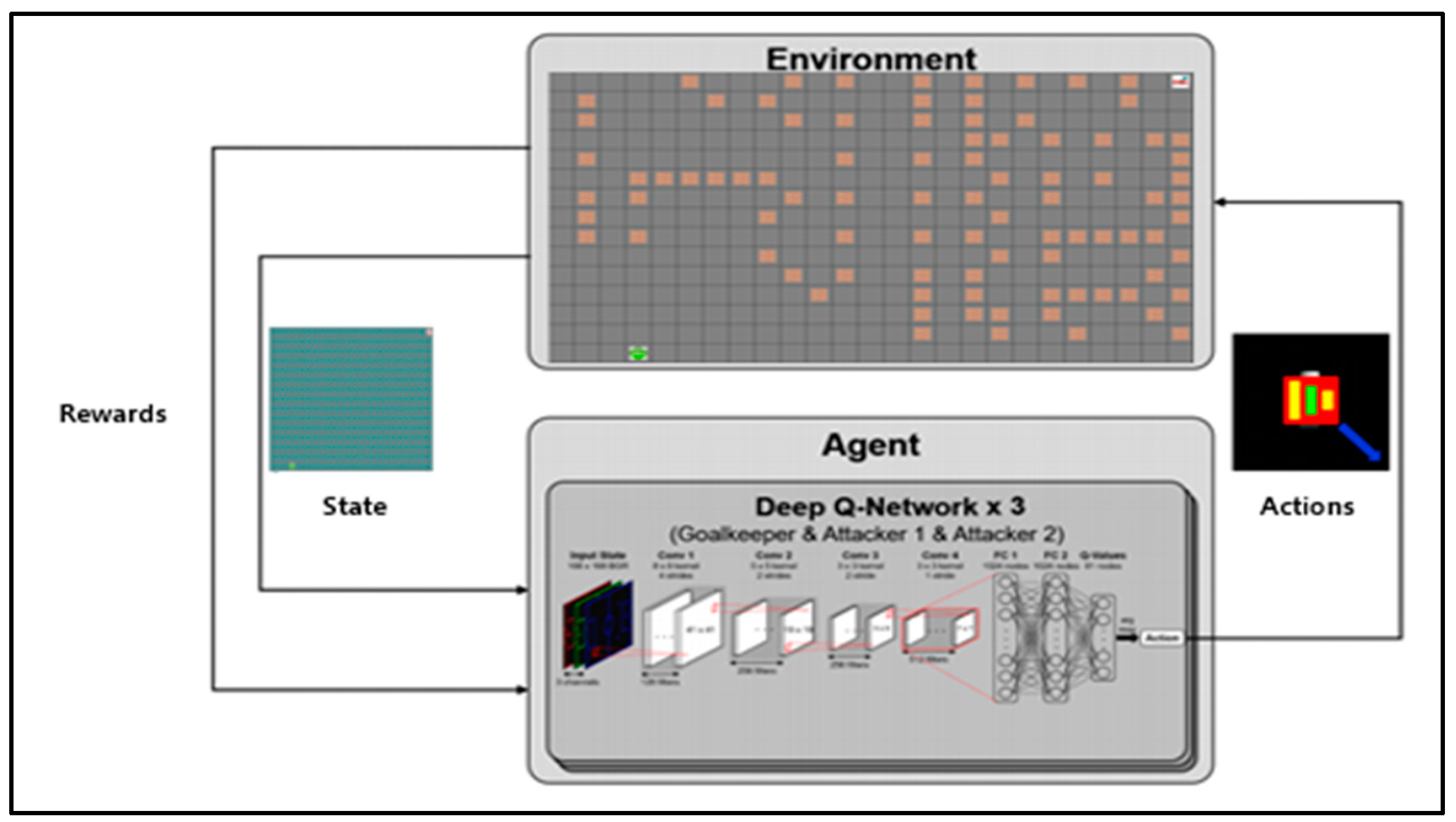
The experiment result compares the proposed algorithm with the existing A* algorithm. The proposed algorithm learns based on the search time of the A* algorithm and assumes learning success when it reaches the target position more quickly than the A* algorithm. Figure 4 shows the simulation configuration diagram of the proposed algorithm. The environmental information image used by CNN is 2560 × 2000 and is designed with 3 × 3 filters with a total of 19 layers (16conv. and 3 FC layers) in the form of VGGNet [42].
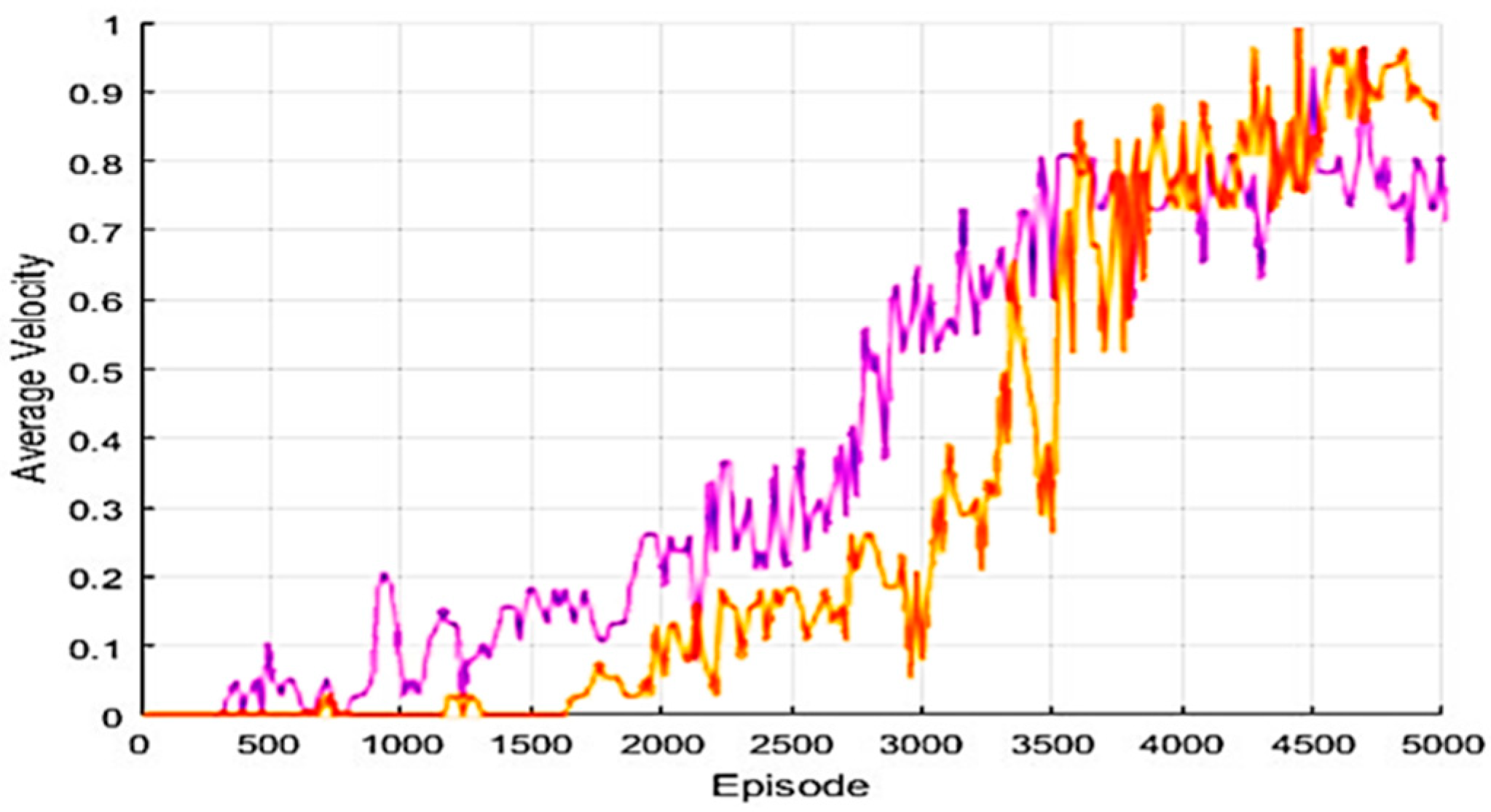
Figure 5 shows the score of the Q parameter when learning by episode. In the graph, the red line depicts the score of the proposed algorithm and the blue line is the score when learning Q parameters per mobile robot. The experiment result confirms that the score of the proposed algorithm is slightly slower at the beginning of learning but reaches the final goal score.
The proposed algorithm, as in Figure 6, which shows the target arrival speed of the episode-based algorithm, has slower learning progression speed than the Q parameter of each model with a similar target position.
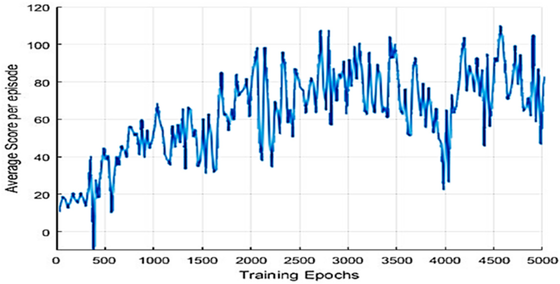
Figure 7 depicts that the average score of each generation increases gradually as learning progresses. As the learning progresses, it gradually gets better results.

4.3. Experimental Results in a Static Environment

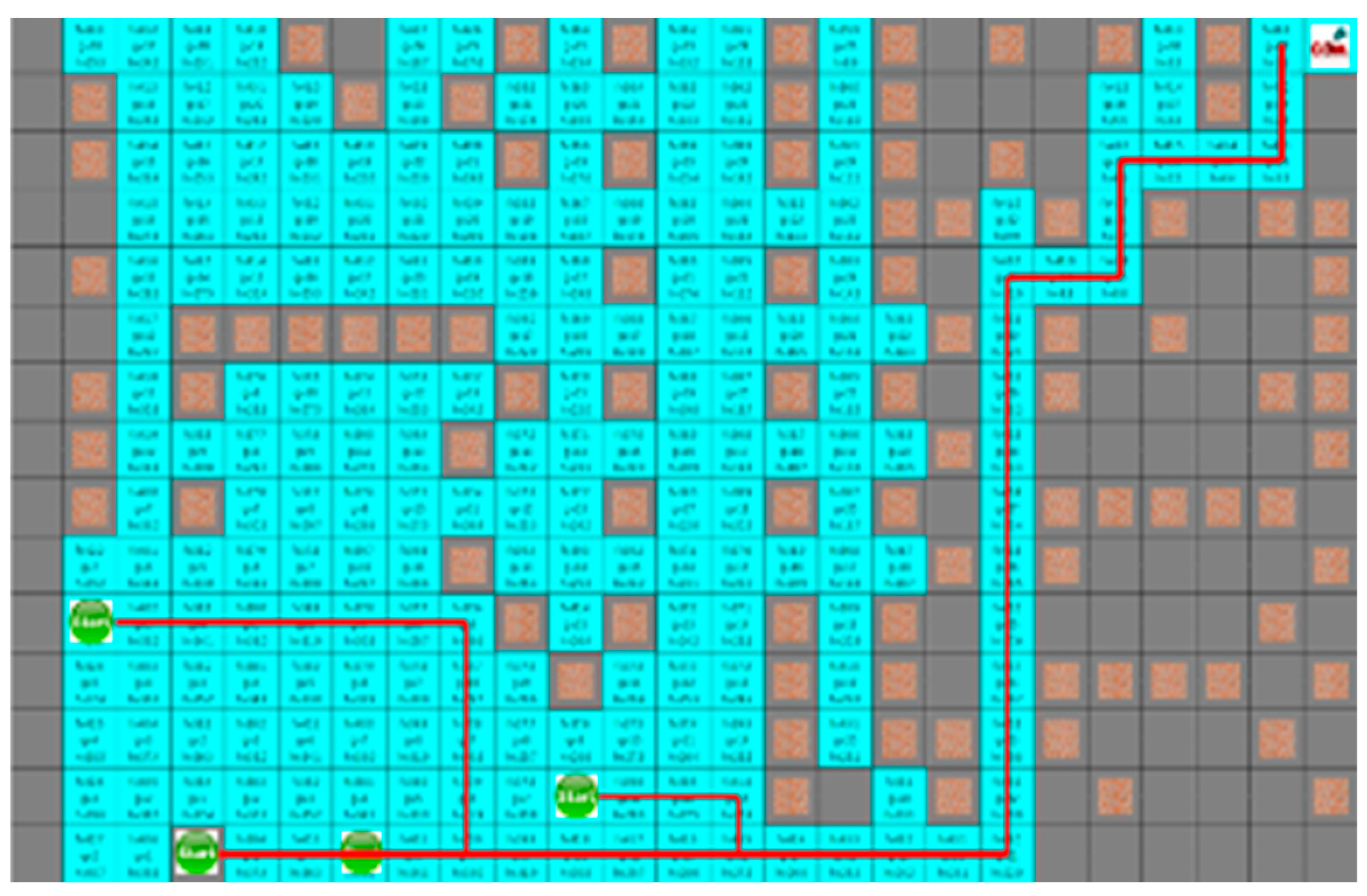
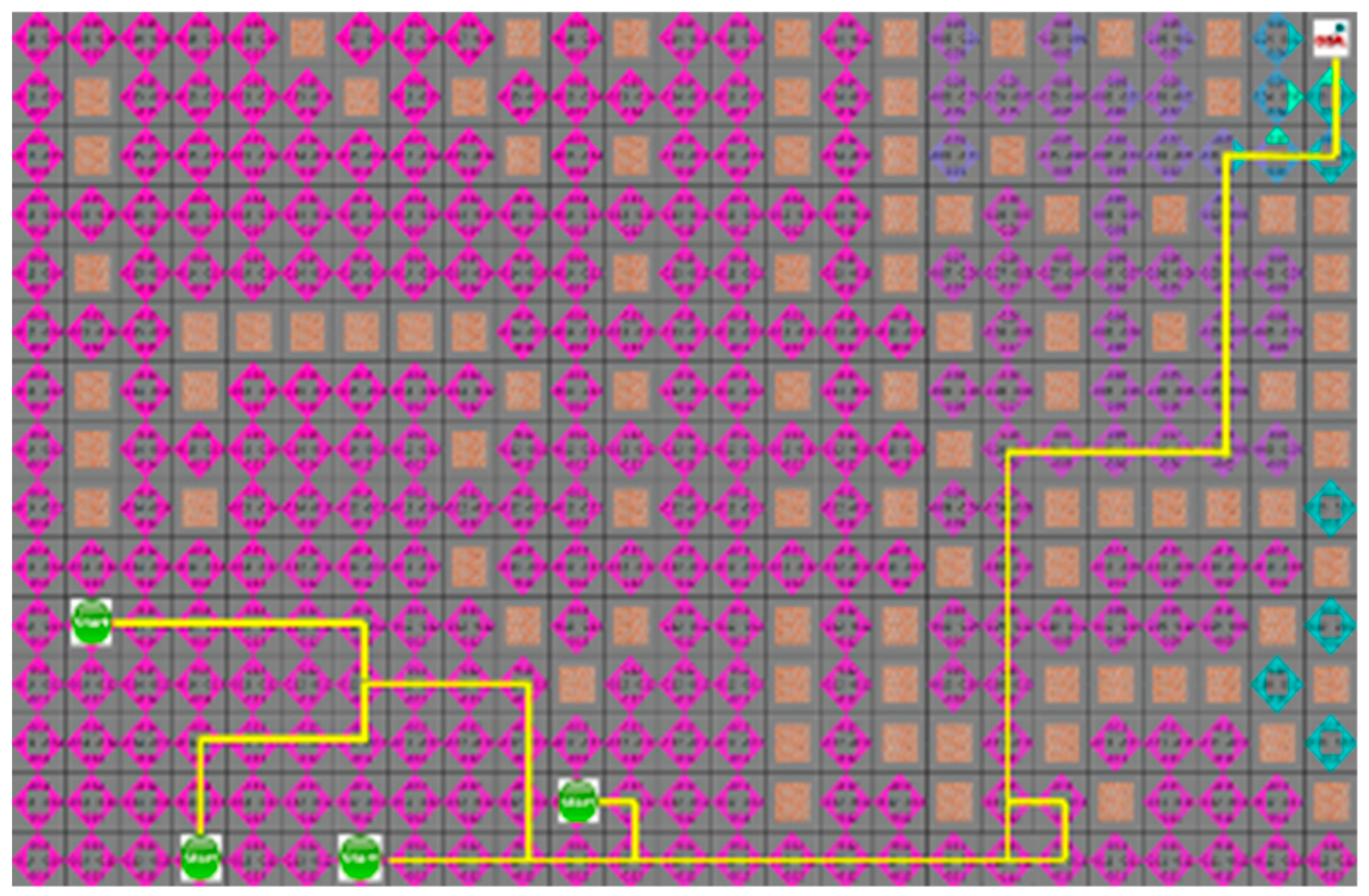
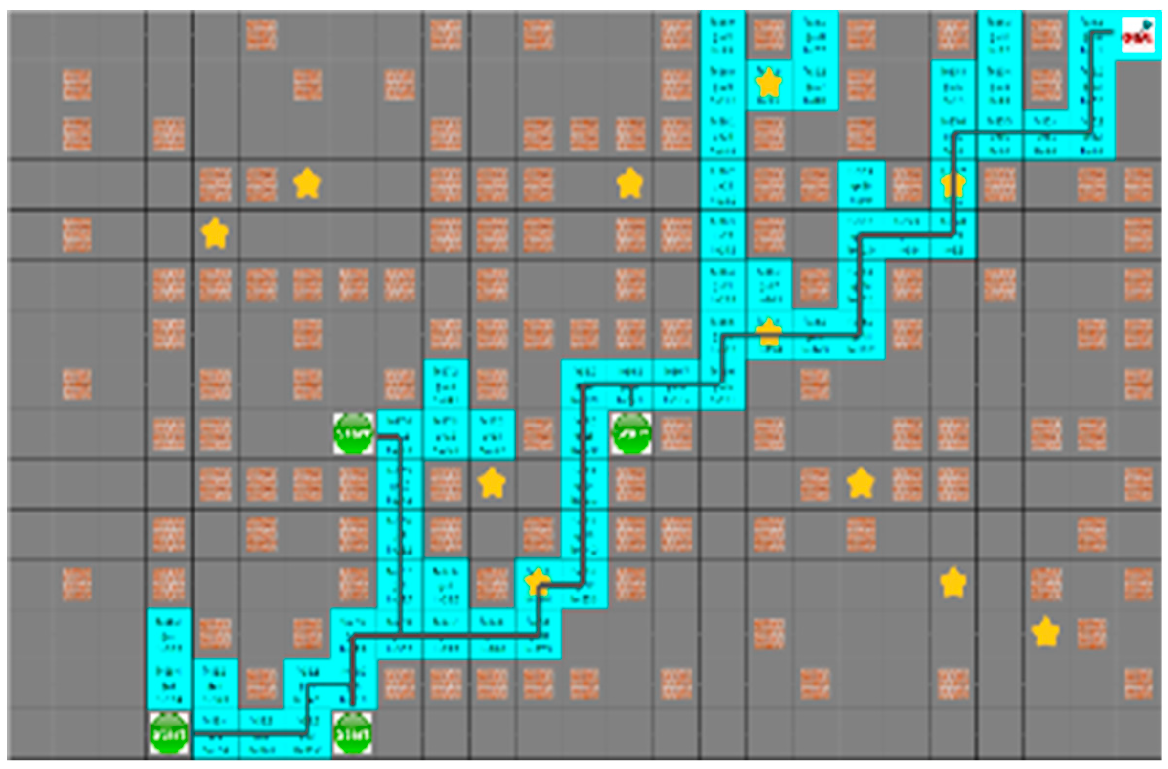
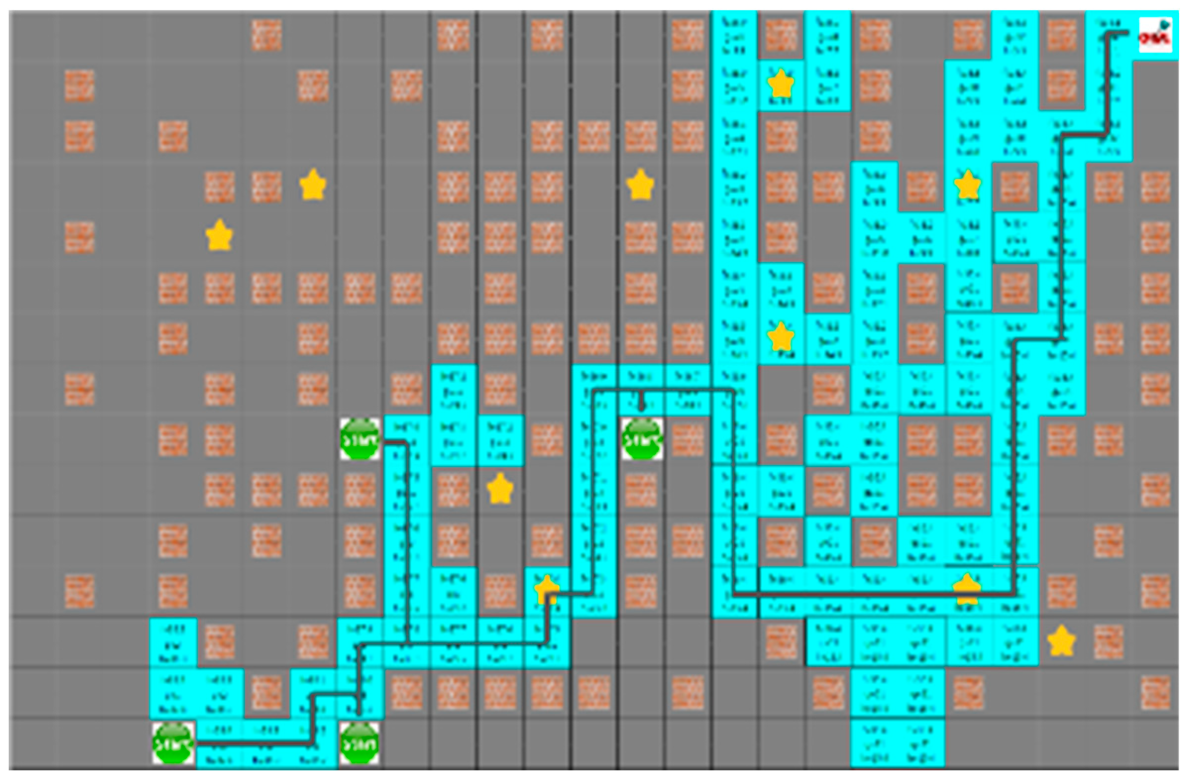
In Section 4.3, the proposed algorithm is compared with the A* algorithm. Because the A* algorithm always finds the shortest path, it can see how quickly the proposed algorithm can find the shortest path. The proposed algorithm and the A* algorithm were tested by four robots to find a path with an arbitrary numbers of obstacles in random initial positions. The test was repeated 100 times on the generated map, which is changed 5000 times to obtain the route visited by the robot and the shortest path for each robot to reach the target point. In the first case, the search area and the time to reach the target point of the proposed algorithm is smaller than the A* algorithm, but the actual travel distance of the robot is increased, as shown in Figure 8 and Figure 9. Figure 8 and Figure 9 depict the results of the A* algorithm and the proposed algorithm, respectively. The average search range of A* algorithm is 222 node visitation. The shortest paths of robots 1 to 4 were 35, 38, 43, and 28 steps, respectively, and the proposed algorithm, where each robot path are 41, 39, 44, and 31 steps, had 137 visited nodes.
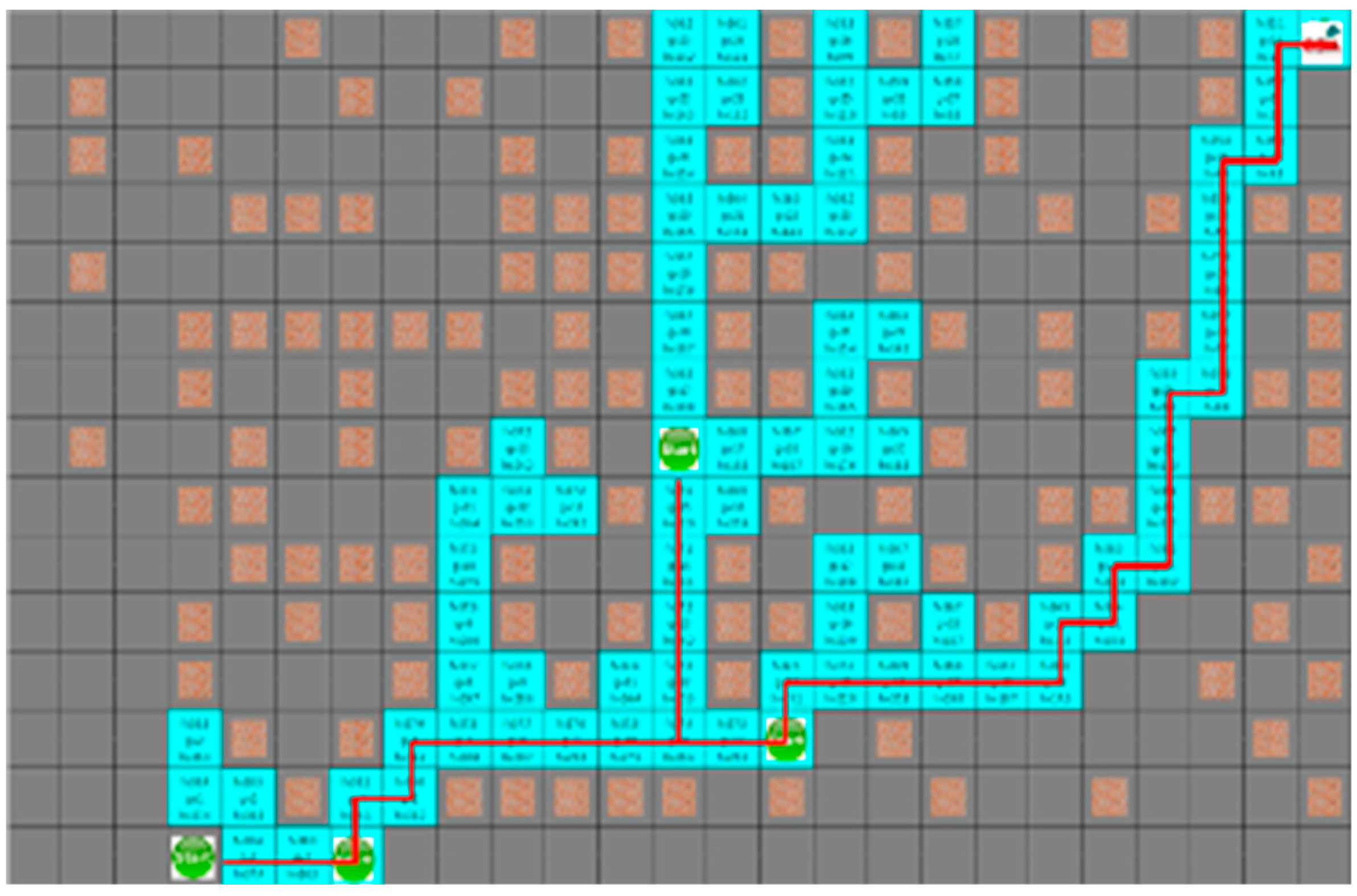
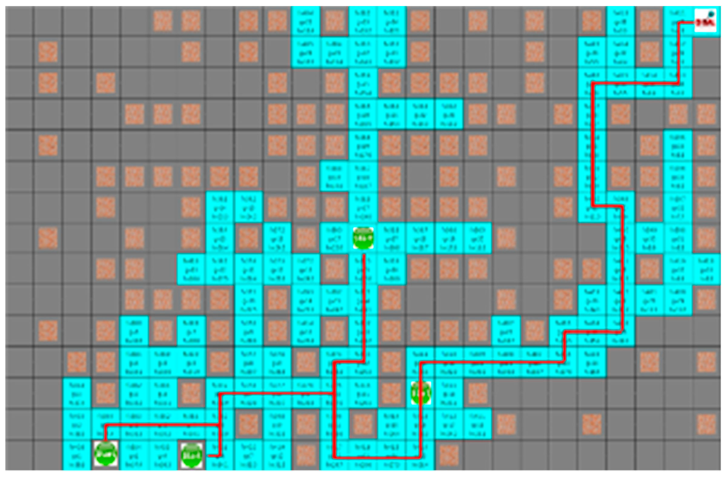
As shown in Figure 10 and Figure 11, which are the result of the A* algorithm and the proposed algorithm, respectively for the second case, the search range of the proposed algorithm is similar to that of the A* algorithm. The average search range of A* algorithm is 80 node visitation. The shortest paths of robots 1 to 4 were 33, 29, 28, and 21 steps, and the proposed algorithm had 65 visited nodes, where each robot pathare 34, 36, 32, and 25 steps, respectively.
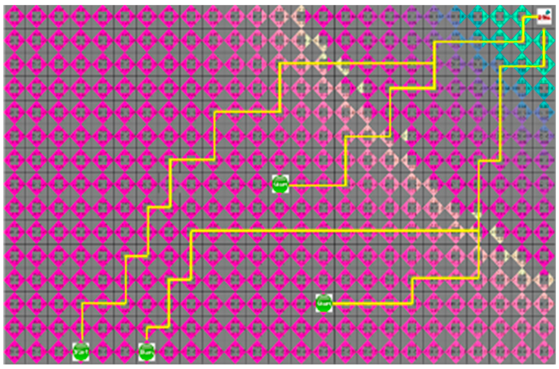
In the third case without obstacles in environment, as shown in Figure 12 and Figure 13, the search range of two algorithms is the same, and the movement path of the robot is similar. The average search range of the A* algorithm was 66 node visitation. The shortest paths of robots 1 to 4 were 33, 29, 28, 21, and 66 steps; the proposed algorithm had 66 visited nodes, and each robot path was 34, 31, 28, and 22 steps, respectively.
In the fourth case, the search range of both algorithms is similar, and the movement path of the robot is the same. Figure 14 and Figure 15 show the results of the A* algorithm and the proposed algorithm, respectively. In the average search range of A* algorithm, robot visited 121 nodes, and the shortest paths of robots 1 to 4 were 40, 38, 36, and 23 steps respectively. And the proposed algorithm had 100 visited nodes, and the shortest path of each robot is 40, 39, 36, and 23 steps, respectively.
Table 1 shows the search range of the proposed algorithm and A* algorithm for each situation. The search range is one of the most important factors on effective robot navigation to the target point. As shown in Table 1, the proposed algorithm has a smaller search range than the A* algorithm.
Table 2 shows the generated path for each robot according to the situation for both proposed and A* algorithm. The proposed algorithm results in no less number of steps than A* in an average generation. In general, A* algorithm is not always searching for the optimal path because it always searches the optimal path in a static environment. However, the proposed algorithm generates the path faster than A*.
Table 3 shows the frequency of occurrence of each situation when a total of 5000 experiments were conducted. Although the search area is small, the situation 1 where the robot generation path is long shows about 58% of occurrence, and the situation 2 where the search area and travel distance are similar is about 34%. According to the simulation result, the search range of the proposed method is always smaller and the robot generation path is the same or similar to the robot path generated by the A* algorithm with a probability of about 34.76%.

4.4. Experimental Results in a Dynamic Environment

Experiments based on the proposed algorithm in a dynamic environment is performed to compare the learning results of the D* algorithm. D* [43] and its variants have been widely used for mobile robot navigation because of its adaptation on dynamic environment. During the navigation of the robot, new information is used for a robot to replan a new shortest path from its current coordinates repeatedly. Under the 5000 different dynamic environments consisting of the smallized static environment as done in Section 4.3, and dynamic obstacles with random initial positions, the simulation was performed around 100 times per environment.
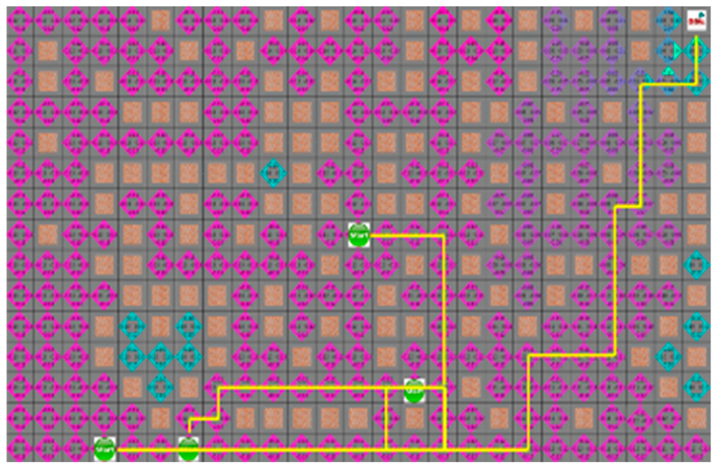
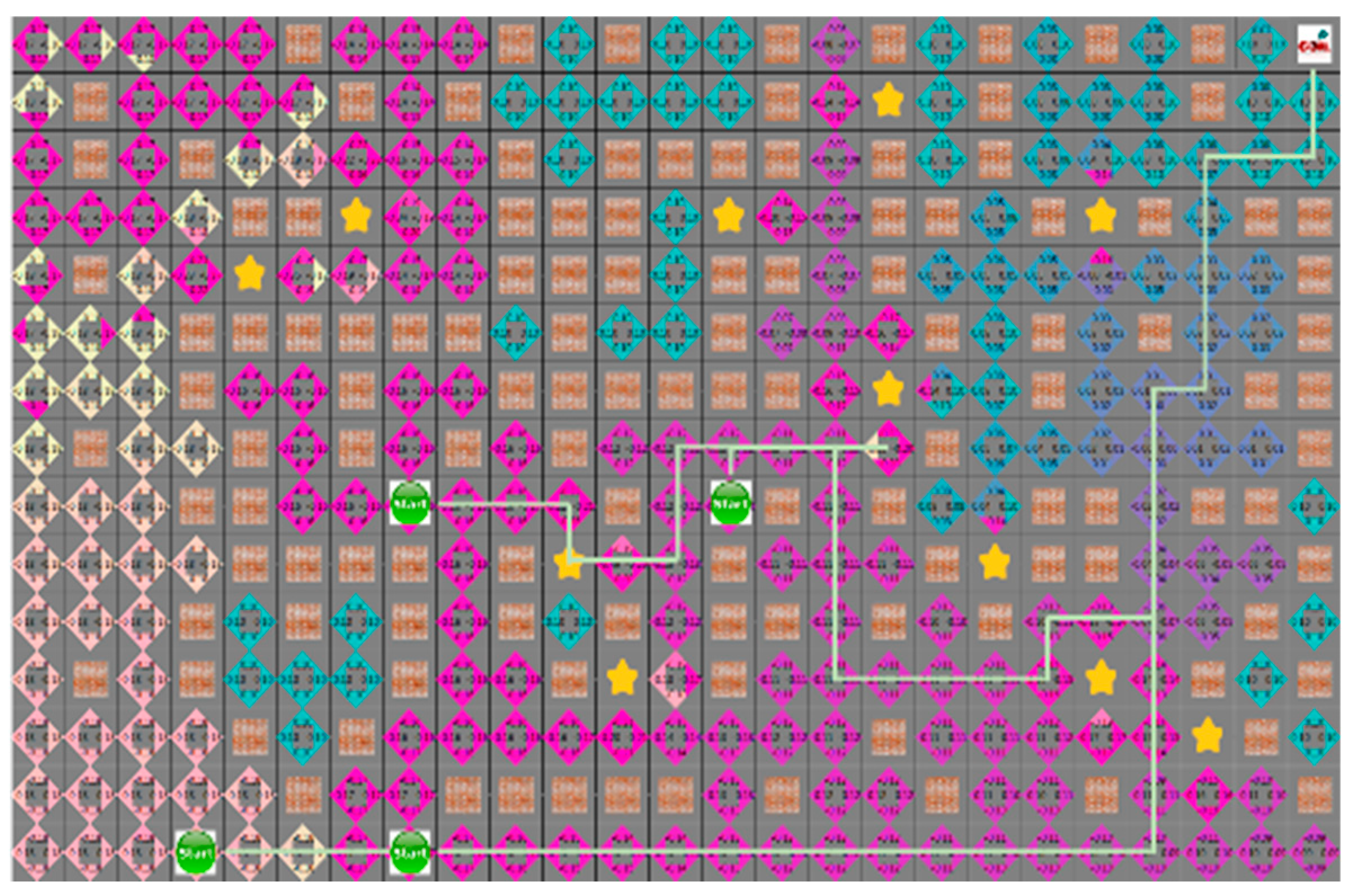
For the D* algorithm, if an obstacle is locates on the robot path, the path will be checked again after the path of movement. In the same situation, different paths may occur depending on the circumstances of the moving obstacle. Figure 16 shows that the yellow star is a dynamic obstacle that creates the shortest path, as shown in Figure 16, or the path to the target point rather than the shortest path, as shown in Figure 17. This shows that the situation of the moving obstacle affects the robot’s path.
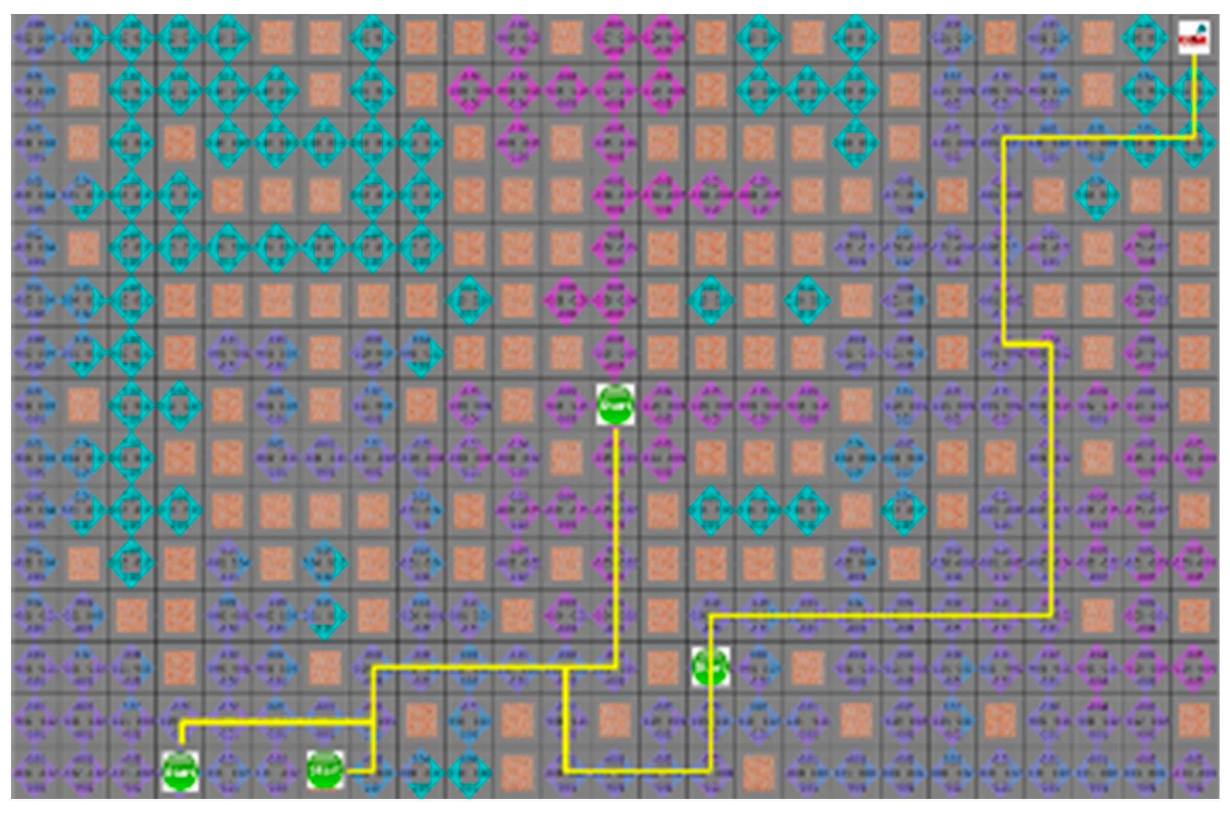
In the proposed algorithm under a dynamic environment where moving obstacles are located on the traveling path of the robot, they do not block the robot, as shown in Figure 18. It guarantees a short traveling distance of each robot.
As shown in Figure 19, the robot moves downward to avoid collision with obstacles on the path of the robot. In Figure 19, the extent to which the path created by D* and the proposed algorithm was not moved to the existing path by the mobile yellow star and explored to generate the bypass path.
Since the robot moves actively to the next position depending on the results learned step by step, it is possible to create a path to the target point in a dynamic environment.
Table 4 shows under a dynamic environment, the first bypass path of D* and the proposed algorithm have 84 and 65 search ranges to move to the target point, respectively. In addition, for the second bypass, each method has 126 and 83 search range, respectively.
Table 5 shows the minimum search range, the maximum search range, and the average search range of the simulation for the D* algorithm and the proposed algorithm for the overall simulation results. All of the three indicators show that the search range of the proposed algorithm is no bigger than D*. Since the search range of the proposed method is small when searching for the bypass path, efficient path planning is possible to the target point. The proposed algorithm used the A* algorithm as a comparison algorithm, which is not available in a dynamic environment. The proposed algorithm was learned by comparing it with the A* algorithm, but unlike the A*, path generation is possible even in a dynamic environment.

5. Conclusions

The problem of multi-robot path planning is motivated by many practical tasks because of its efficiency for performing given missions. However, since each robot in the group operates individually or cooperatively depending on the situation, the search area of each robot is increased. Reinforcement learning in the robot’s path planning algorithm is mainly focused on moving in a fixed space where each part is interactive.
The proposed algorithm combines the reinforcement learning algorithm with the path planning algorithm of the mobile robot to compensate for the demerits of conventional methods by learning the situation where each robot has mutual influence. In most cases, existing path planning algorithms are highly depends on the environment. Although the proposed algorithm used an A* algorithm that could not be used in a dynamic environment as a comparison algorithm, it also showed that path generation is possible even in a dynamic environment. The proposed algorithm is available for use in both a static environment and in a dynamic environment. Since robots share the memory used for learning, they learn the situation by using one system. Because learning is slow and the result includes errors of each robot at the beginning of learning, each robot has the same result as using each parameter after learning progress to a certain extent. The proposed algorithm including A* for learning can be applied in real robots by minimizing the memory to store the operations and values.
A* algorithm always finds the shortest distance rather than the search time. Under the proposed algorithm, which shows diverse results, the search area of each robot is similar to A*-based learning. However, in the environment where the generated path is simple or without obstacles, an unnecessary movement occurs. To enhance the proposed algorithm, research on the potential field algorithm is undergoing. In addition, the proposed algorithm did not take into account the dynamics of robots and obstacles [44,45,46] and performed simulations in situations in which robots and obstacles always made ideal movements without taking into account the dynamics of them. Based on the simulation result, the research considering the actual environment and physical engine is on the way.

Author Contributions

Conceptualization, H.B.; software, H.B. and G.K; validation, J.K., D.Q., and G.K.; data curation, J.K.; writing—original draft preparation, H.B.; writing—review and editing, D.Q.; visualization, G.K.; supervision, S.L.; project administration, S.L.

Funding

This work was supported by the Basic Science Research Program, through the National Research Foundation of Korea, Ministry of Science, under Grant 2017R1D1A3B04031864.

Conflicts of Interest

The authors declare no conflict of interest.

References

  1. Nasser, M. Pattern Recognition and Machine Learning. J. Electron. Imaging 2007, 16, 4. [Google Scholar]
  2. Yu, D.; Li, D. Deep learning and its applications to signal and information processing [exploratory dsp]. IEEE Signal Process. Mag. 2010, 28, 145–154. [Google Scholar] [CrossRef]
  3. Hinton, G.; Deng, L.; Yu, D.; Dahl, G.E.; Mohamed, A.R.; Jaitly, N.; Kingsbury, B. Deep neural Networks for acoustic modeling in speech recognition. IEEE Signal Process. Mag. 2012, 29, 82–97. [Google Scholar] [CrossRef]
  4. Graves, A.; Abdel-rahman, M.; Geoffrey, H. Speech recognition with deep recurrent neural networks. In Proceedings of the 2013 IEEE International Conference on Acoustics, Speech and Signal Processing, Vancouver, BC, Canada, 26–31 May 2013; pp. 6645–6649. [Google Scholar]
  5. Kumar, A. Ask me anything: Dynamic memory networks for natural language processing. In Proceedings of the International Conference on Machine Learning, New York, NY, USA, 19–24 June 2016; pp. 1378–1387. [Google Scholar]
  6. Machine Learning and Natural Language Processing. Available online: http://l2r.cs.uiuc.edu/~danr/Teaching/CS546-13/Papers/marquez-LNLP00.pdf (accessed on 11 July 2010).
  7. Manning, C. The Stanford CoreNLP natural language processing toolkit. In Proceedings of the 52nd Annual Meeting of the Association for Computational Linguistics: System Demonstrations, Baltimore, MD, USA, 22–27 June 2014; pp. 55–60. [Google Scholar]
  8. Collobert, R.; Jason, W. A unified architecture for natural language processing: Deep neural networks with multitask learning. In Proceedings of the 25th International Conference on Machine Learning, Helsinki, Finland, 5–9 July 2008; pp. 160–167. [Google Scholar]
  9. Kononenko, I. Machine learning for medical diagnosis: History, state of the art and perspective. Artif. Intell. Med. 2001, 23, 89–109. [Google Scholar] [CrossRef]
  10. Shvets, A.A.; Rakhlin, A.; Kalinin, A.A.; Iglovikov, V.I. Automatic instrument segmentation in robot-assisted surgery using deep learning. In Proceedings of the 2018 17th IEEE International Conference on Machine Learning and Applications (ICMLA), Orlando, FL, USA, 17–20 December 2018; pp. 624–628. [Google Scholar]
  11. Bottou, L. Large-scale machine learning with stochastic gradient descent. In Proceedings of the COMPSTAT’2010, Paris, France, 22–27 August 2010; pp. 177–186. [Google Scholar]
  12. Peters, J.; Stefan, S. Natural actor-critic. Neurocomputing 2008, 71, 1180–1190. [Google Scholar] [CrossRef]
  13. Bhasin, S.; Kamalapurkar, R.; Johnson, M.; Vamvoudakis, K.G.; Lewis, F.L.; Dixon, W.E. A novel actor-identifier architecture for approximate optimal control of uncertain nonlinear systems. Automatica 2013, 49, 82–92. [Google Scholar] [CrossRef]
  14. Vamvoudakis Kyriakos, G.; Frank, L.L. Online actor-critic algorithm to solve the continuous-time infinite horizon optimal control problem. Automatica 2010, 46, 878–888. [Google Scholar] [CrossRef]
  15. Florensa, C.; Degrave, J.; Heess, N.; Springenberg, J.T.; Riedmiller, M. Self-supervised learning of image embedding for continuous control. arXiv 2019, arXiv:1901.00943. [Google Scholar]
  16. Lillicrap Timothy, P. Continuous control with deep reinforcement learning. arXiv 2015, arXiv:1509.02971. [Google Scholar]
  17. Watkins Christopher, J.; Peter, D. Q-learning. Mach. Learn. 1992, 8, 279–292. [Google Scholar] [CrossRef]
  18. Littman, M.L. Markov games as a framework for multi-agent-reinforcement learning. In Proceedings of the Eleventh International Conference on Machine Learning, New Brunswick, NJ, USA, 10–13 July 1994; Volume 157, pp. 157–163. [Google Scholar]
  19. Foster, D.; Peter, D. Structure in the space of value functions. Mach. Learn. 2002, 49, 325–346. [Google Scholar] [CrossRef]
  20. Kofinas, P.; Dounis, A.I.; Vouros, G.A. Fuzzy Q-Learning for multi-agent decentralized energy management in microgrids. Appl. Energy 2018, 219, 53–67. [Google Scholar] [CrossRef]
  21. Keselman, A.; Ten, S.; Ghazali, A.; Jubeh, M. Reinforcement Learning with A* and a Deep Heuristic. arXiv 2018, arXiv:1811.07745. [Google Scholar]
  22. Stentz, A. Optimal and efficient path planning for partially known environments. In Intelligent Unmanned Ground Vehicles; Springer: Boston, MA, USA, 1997; pp. 203–220. [Google Scholar]
  23. Ge, S.S.; Yan, J.C. New potential functions for mobile robot path planning. IEEE Trans. Robot. Autom. 2000, 16, 615–620. [Google Scholar] [CrossRef] [Green Version]
  24. Zhang, Y.; Gong, D.-W.; Zhang, J.-H. Robot path planning in uncertain environment using multi-objective particle swarm optimization. Neurocomputing 2013, 103, 172–185. [Google Scholar] [CrossRef]
  25. Tharwat, A.; Elhoseny, M.; Hassanien, A.E.; Gabel, T.; Kumar, A. Intelligent Bézier curve-based path planning model using Chaotic Particle Swarm Optimization algorithm. Clust. Comput. 2018, 1–22. [Google Scholar] [CrossRef]
  26. Elhoseny, M.; Tharwat, A.; Hassanien, A.E. Bezier curve based path planning in a dynamic field using modified genetic algorithm. J. Comput. Sci. 2018, 25, 339–350. [Google Scholar] [CrossRef]
  27. Hu, X.; Chen, L.; Tang, B.; Cao, D.; He, H. Dynamic path planning for autonomous driving on various roads with avoidance of static and moving obstacles. Mech. Syst. Signal Process. 2018, 100, 482–500. [Google Scholar] [CrossRef]
  28. Alomari, A.; Comeau, F.; Phillips, W.; Aslam, N. New path planning model for mobile anchor-assisted localization in wireless sensor networks. Wirel. Netw. 2018, 24, 2589–2607. [Google Scholar] [CrossRef]
  29. Li, G.; Chou, W. Path planning for mobile robot using self-adaptive learning particle swarm optimization. Sci. China Inf. Sci. 2018, 61, 052204. [Google Scholar] [CrossRef]
  30. Thrun, S.; Wolfram, B.; Dieter, F. A real-time algorithm for mobile robot mapping with applications to multi-robot and 3D mapping. In Proceedings of the ICRA, San Francisco, CA, USA, 24–28 April 2000; Volume 1, pp. 321–328. [Google Scholar]
  31. Bruce, J.; Manuela, V. Real-time randomized path planning for robot navigation. In Proceedings of the IEEE/RSJ International Conference on Intelligent Robots and Systems, Takamatsu, Japan, 31 October–5 November 2002; Volume 3, pp. 2383–2388. [Google Scholar]
  32. Indelman, V. Cooperative multi-robot belief space planning for autonomous navigation in unknown environments. Auton. Robot. 2018, 42, 353–373. [Google Scholar] [CrossRef]
  33. Fan, T.; Long, P.; Liu, W.; Pan, J. Fully distributed multi-robot collision avoidance via deep reinforcement learning for safe and efficient navigation in complex scenarios. arXiv 2018, arXiv:1808.03841. [Google Scholar]
  34. Van Den Berg, J.; Dave, F.; James, K. Anytime path planning and replanning in dynamic environments. In Proceedings of the 2006 IEEE International Conference on Robotics and Automation, Orlando, FL, USA, 15–19 May 2006; pp. 2366–2371. [Google Scholar]
  35. Raja, P.; Sivagurunathan, P. Optimal path planning of mobile robots: A review. Int. J. Phys. Sci. 2012, 7, 1314–1320. [Google Scholar] [CrossRef]
  36. Van, H.; Hado, A.G.; David, S. Deep reinforcement learning with double q-learning. In Proceedings of the Thirtieth AAAI Conference on Artificial Intelligence, Phoenix, AZ, USA, 12–17 February 2016. [Google Scholar]
  37. Mnih, V. Playing atari with deep reinforcement learning. arXiv 2013, arXiv:1312.5602. [Google Scholar]
  38. Mnih, V. Asynchronous methods for deep reinforcement learning. In Proceedings of the International Conference on Machine Learning, New York, NY, USA, 19–24 June 2016; pp. 1928–1937. [Google Scholar]
  39. Ren, S. Faster r-cnn: Towards real-time object detection with region proposal networks. In Proceedings of the Twenty-ninth Conference on Neural Information Processing Systems, Montréal, QC, Canada, 7–12 December 2015; pp. 91–99. [Google Scholar]
  40. Kalchbrenner, N.; Edward, G.; Phil, B. A convolutional neural network for modelling sentences. arXiv 2014, arXiv:1404.2188. [Google Scholar]
  41. Abdel-Hamid, O. Convolutional neural networks for speech recognition. IEEE/ACM Trans. Audio Speech Lang. Process. 2014, 22, 1533–1545. [Google Scholar] [CrossRef]
  42. Simonyan, K.; Zisserman, A. Very deep convolutional networks for large-scale image recognition. arXiv 2014, arXiv:1409.1556. [Google Scholar]
  43. Hart, P.E.; Nilsson, N.J.; Raphael, B. A formal basis for the heuristic determination of minimum cost paths. IEEE Trans. Syst. Sci. Cybern. 1968, 4, 100–107. [Google Scholar] [CrossRef]
  44. Borboni, A.; Lancini, M. Commanded motion optimization to reduce residual vibration. J. Vib. Acoust. 2015, 137, 031016. [Google Scholar] [CrossRef]
  45. Alonso-Mora, J.; Montijano, E.; Nägeli, T.; Hilliges, O.; Schwager, M.; Rus, D. Distributed multi-robot formation control in dynamic environments. Auton. Robots 2019, 43, 1079–1100. [Google Scholar] [CrossRef]
  46. Yu, J.; Ji, J.; Miao, Z.; Zhou, J. Neural network-based region reaching formation control for multi-robot systems in obstacle environment. Neurocomputing 2019, 333, 11–21. [Google Scholar] [CrossRef]
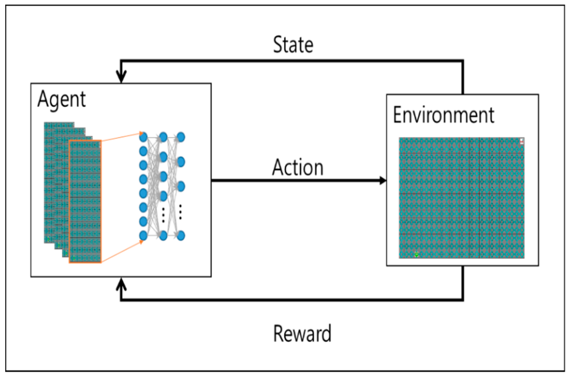
Figure 1. Q Learning concept.
Applsci 09 03057 g001
Figure 2. The concept of the proposed algorithm.
Applsci 09 03057 g002
Figure 3. Simulation environment.
Applsci 09 03057 g003
Figure 4. Simulation configuration diagram of proposed algorithm.
Applsci 09 03057 g004
Figure 5. Score depending on algorithms according to episode.
Applsci 09 03057 g005
Figure 6. The rate at which episode goals are reached.
Applsci 09 03057 g006
Figure 7. The rate of reaching the goal by Epochs.
Applsci 09 03057 g007
Figure 8. The simulation result of A* algorithm for the first situation.
Applsci 09 03057 g008
Figure 9. The simulation result of proposed algorithm for the first situation.
Applsci 09 03057 g009
Figure 10. The simulation result of A* algorithm for the second situation.
Applsci 09 03057 g010
Figure 11. The simulation result of proposed algorithm for the second situation.
Applsci 09 03057 g011
Figure 12. The simulation result of A* algorithm result for the third situation.
Applsci 09 03057 g012
Figure 13. The simulation result of proposed algorithm for the third situation.
Applsci 09 03057 g013
Figure 14. The simulation result of A* algorithm for the fourth situation.
Applsci 09 03057 g014
Figure 15. The simulation result of proposed algorithm for the fourth situation.
Applsci 09 03057 g015
Figure 16. The shortest path generated without collision with dynamic obstacles using D*.
Applsci 09 03057 g016
Figure 17. Path using D* in a mobile obstacle environment the route returned by an obstacle.
Applsci 09 03057 g017
Figure 18. The generated path using proposed algorithm in dynamic environment.
Applsci 09 03057 g018
Figure 19. Robot bypass path generation using the proposed algorithm in dynamic environment.
Applsci 09 03057 g019
Table 1. The average search range of A* and the proposed algorithm.
SituationA* AlgorithmProposed Algorithm
Situation 1258155
Situation 28367
Situation 36969
Situation 4120101
Table 2. The robot average generation path of A* and the proposed algorithm.
SituationA* AlgorithmProposed Algorithm
Situation 13536
Situation 22830
Situation 33031
Situation 43232
Table 3. Frequency of occurrence by situation.
SituationFrequency of Occurrence
Situation 13262
Situation 21556
Situation 3102
Situation 480
Table 4. Total search scope under dynamic environment for D* and proposed algorithm.
SituationD* AlgorithmProposed Algorithm
First bypass8465
Second bypass12683
Table 5. Minimum, maximum, and average exploration range during the full simulation of D* and proposed algorithms.
SituationD* AlgorithmProposed Algorithm
Minimum Exploration Range6666
Maximum Exploration Range294237
Average Exploration Range188141