Abstract
Flow measurements in open channels have often utilized velocity-area methods. Thus, estimations of the average velocity in a cross-section of rural canals play an important role in the flow measurement of an irrigation district. This paper derives a model for calculating depth average velocity. This model considers the classical logarithmic formula describing the velocity distribution and flow partitioning theory, which is aimed at finding out a location that represents the depth average velocity (LDAV) along the vertical line from boundary to water surface. Subsequently, the average flow velocity of the whole channel can be further determined by using the velocity-area method in different regions. Moreover, the LDAV has different expressions in different sub-regions according to flow partitioning theory under various aspect ratios. The results are verified by experiments under different experimental conditions, and the formula is highly applicable and has a high theoretical significance and practical value.
1. Introduction
The measurement of irrigation water consumption in irrigation districts is significant in the implementation of a stringent water resources management system [1]. Rural canals can be approximated by rectangular open channels. The standard method for calculating discharge in an open channel is the velocity-area method, which requires velocity measurements to be made at many points throughout the area. Although this method is considered to be particularly reliable, a large number of measurements results in an associated time cost of measurement. Numerous researchers [2] have sought to define methods for estimating discharge on the basis of an extremely reduced number of velocity observations. One important approach in this respect is to estimate the discharge by measuring the velocity at a point which stands for the depth average velocity on a vertical measuring profile. However, there is no relevant research on how to obtain the location of this point. For practical reasons, it is helpful to separate the flow regions and to separate the bed or side-wall local friction velocity, which is crucial for velocity distribution. It is universally acknowledged that the flow partitioning theory is extremely important for velocity distribution. Nevertheless, the usual application of the flow partitioning theory is in calculating the shear stress in a practical channel. Thus, how to use the flow partitioning theory to find a point which stands for the average velocity on a vertical measuring profile has provoked researchers’ interest [3]. The depth average velocity of natural rivers is the basis for studying sediment movement and riverbed evolution, and it has been a key issue in hydraulics for a long time, which is directly related to its function in the calculation of cross-sectional flow and the longitudinal dispersion coefficient [4]. The study of velocity distribution is critical to the calculation of the depth average velocity.
There have been many studies on velocity distribution. In 1938, Keulegan [5] proposed that a logarithmic expression can be used to describe the average velocity distribution of fully developed uniform turbulence in open channels:
where , , , is frictional velocity, is the coefficient of kinematic viscosity, and are constants, and is the Karman constant.
Coles [6] proposed a wake function to explain the turbulent boundary layer flow development process:
where is the wake function.
Further more, Coles proposed that the wake function can correct the deviation of logarithmic functions of the velocity distribution of a two-dimensional incompressible turbulent boundary layer flow near the water surface:
Nikuradse [7] made an artificial sand rough pipe by using pasting sand with a uniform particle size on the wall of a pipe. The analysis of the experimental data of the smooth sand tube showed that the values of parameters k and B in logarithmic law are 0.4 and 5.5, as shown in Equation (4):
However, with the deepening of understanding in this research area, researchers have developed different views on the scope of the applications of logarithmic law. As the description of logarithmic law near the water surface is not perfect, some scholars have begun to try and find a more consistent functional form to describe the velocity distribution in the whole water depth. Hu [8] conducted experiments which showed that the velocity distribution on the same vertical line turns out to be different with an increasing water depth in different water depth ranges.
Additionally, according to the distribution characteristics of velocity in different water depth ranges, the whole water depth should be divided into three parts: the inner area, the outer area and the surface area. Shiono and Knight [9] integrated the N-S equation along the flow direction to take the average value along the water depth and proposed the Shiono and Knight Model (SKM), which is most widely used in the calculation of the average flow velocity in the cross section of a compound channel. The research conducted by different researchers [10] shows that logarithmic law could be used on velocity distributions of open channel flows. However, under various conditions, there is no agreement on whether the vertical velocity correlation of the cross-section can be expressed using a unified correlation or not.
The Division of flow region for 3-D channel flows has been shown in a number of textbooks on hydraulics [11]. Keulegan [5] is the first to mention the need to divide the flow cross-sectional area into different sections. For turbulence in a prismatic channel, Einstein [12] suggested that the shear force applied to the bed should be separated from the shear force applied to the lateral boundary. Chien and Wan [13] briefly explained the physical meaning of Einstein’s thoughts, and reported that the residual energy in the mainstream should be transferred and eventually dissipated as heat at the boundary. Additionally, the energy in any unit flow is transported to the nearest boundary. In fact, all of these provide an excellent approach to calculating the shear stress in a cross-section. However, the most important issue is whether it is possible to use flow partitioning theory to obtain local frictional velocity separately in different regions. Hydraulic engineers use the concept of flow region division to assume that there is no shear force on the dividing line and have proposed various methods for dividing the cross-section of the channel. They have different views on the division of flow area, and various models have been proposed to express the division lines:
Keulegan Method (KM): Keulegan [5] proposed that the flow in a polygonal channel could be separated into three separate areas, and this is achieved by division lines bisecting the base angles, as shown in Figure 1. Unfortunately, no theoretical explanation for this treatment was provided by the authors.
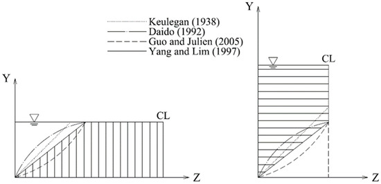
Figure 1.
Different views on the division of the flow region.
Daido Method (DM): Daido [14] performed extensive research to derive an equation for the division lines of a rectangular open channel. The author applied the Karman–Prandtl velocity equation from the sidewall and bed for each dashed line shown in Figure 1. However, the validation of Daido’s model in-flow has not been verified by experimental data.
Guo and Julien Method (GJM): Guo and Julien [15] determined the bed and sidewall shear stresses in a rectangular open channel flow by solving the continuity and momentum equations. Conformal mapping was used to partition the flow and the equation for division lines was derived. The GJM method considers the control volume partitioned by the curved division lines by their first approximation, as illustrated in Figure 1.
Yang and Lim Method (YLM): Their work has been widely quoted in many textbooks and has had a great impact on fluid mechanics. Yang and Lim [16] proposed that there is a slanted straight line, which can be used to divide the cross-section into two different flow regions, as shown in Figure 1.
There have been many ways to obtain the average velocity in a cross-section of an open channel. However, the flow division theory has almost never been applied to obtain the average velocity in open rectangular channels. It is very important to find out where the characteristic point is, which stands for the average velocity along the normal line of boundary. This article aims to formulate a correlation for finding out the characteristic point standing for the average depth velocity along the normal line from the boundary wall of the channel and validate the correlation based upon experiments.
2. Materials and Methods
Han [17] demonstrated the existence of a dividing line in a smooth channel flow with a smooth flat or curved bed by analyzing the average velocity distribution, which can be used to obtain the velocity distribution in different flow areas. In order to understand how flow division theory affects the velocity distribution, Prandtl’s theory needs to be revisited. Prandtl [18] proposed the concept of mixing length to express eddy viscosity.
Prandtl assumed that the mixing length is directly proportional to the distance from the boundary, , where is the Karman constant. Generally, the value of is 0.4. Under different conditions, the value of may be different [16]. Substituting the boundary conditions and into Equation (6), the equation for velocity is obtained.
where is the frictional velocity, and may be related to local velocity of the sticky lower layer, according to Equation (8).
where c is the coefficient measured by experiments, and is the local friction, which may be different from .
Therefore, if a flow region can be divided, then the local shear stress can be used, which can better reflect the actual side wall effect instead of the concept of average shear stress. Additionally, the local boundary shear stress may be determined using Equations (9) and (10).
where is the vertical distance from the boundary to the boundary line, as proposed by Yang and Lim [15].
According to YLM, the division line in a rectangular open channel can be expressed using Equation (11):
where z and y are normal to the boundary and k is the slope of division line. Furthermore, k is calculated using Equations (12) or (13).
or
where h is the depth of water, b is the width of the channel, and α is the critical aspect ratio (width to depth ratio), which is equal to 2 in Yang and Lim’s theory.
For a steady, uniform, and fully developed turbulent flow, the classical formulation which can describe the velocity distribution is a logarithmic function that increases from zero velocity at the boundary of the channel and reaches its maximum at the water surface. The velocity distribution can be expressed using Equations (14) and (15).
where u is the flow velocity, is the frictional velocity, which is given by the correlation: and is the local frictional velocity, where g is the gravitational acceleration, s is the energy slope and is the distance from the division line to the boundary. Furthermore, y/z is the distance to the boundary, v is the dynamic viscosity, and B is an empirical coefficient, which is usually equal to 5.5.
According to Yang and Lim’s theory, the flow region can be divided according to the schematic shown in Figure 2 (aspect ratio > 2). Furthermore, the three regions can be defined in half cross-section.
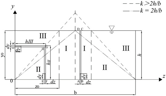
Figure 2.
Flow partition in a rectangular channel (k stands for the slope of division line, k > 2h/b and k = 2h/b).
There is a rectangular channel, whose depth and width are h and b, respectively. According to the flow partition theory and the value of h/b, the three partitions can be determined.
2.1. Division Lines Cross above and on the Water Surface
In this condition, the flow area can be partitioned into three regions—Regions I, II and III—as shown in Figure 2. In Region I, since both dy and dz (in Figure 2) are close to infinitesimal, a point belonging to this infinitesimal rectangle can be substituted for rectangle ABCD. Therefore, the velocity of any point in the flow area can be used to estimate the discharge of this infinitesimal rectangle. Additionally, the discharge can be expressed using Equation (16).
where dQ is the discharge of infinitesimal flow area, and v is the longitudinal velocity of any point in the flow area.
In order to obtain the discharge of this flow area, y is integrated and Equation (17) is obtained.
Therefore, the average velocity of this flow area is obtained from the value of Q/A, where A represents the rectangular cross-sectional area (A = hdz). Furthermore, the velocity can be expressed using Equation (18).
As the velocity distribution is continuous, an equation can be used to obtain the y value of the point, which stands for the average velocity. Combining Equations (14) and (18) will give Equation (19).
By solving this equation, the y value of the point is obtained, which is expressed using Equation (20).
Equation (20) is used to calculate the depth of the point, which stands for the average velocity of the rectangle ABCD in Region I.
Similarly, the y value of the point has to be determined, which stands for the average velocity of two rectangular areas (they can be regarded as rectangles if GH approaches zero) whose lengths are hII and hIII, respectively, and pass through Regions II and III (EFGH and GHIK, respectively, in Figure 2). According to the flow division theory, Equation (14) should be used in Region II, and Equation (15) in Region III. Therefore, the velocity distribution in Region II is different from the velocity distribution in Region III. It is difficult to directly calculate the value of Q of a rectangular area through Regions II and III. For Region II, hII can be regarded as h in Region I, as a result of which the result can be used in Region I to obtain the value of y at the point, which stands for average velocity, whose length is hII and width is dz. It can be expressed using Equation (21).
The rectangular area has the length and width of hIII and dy, respectively, in Region III, where hIII is the distance from the dividing line to the boundary. An infinitesimal rectangle with the length and width of dy and dz (respectively) in the area is assumed. The discharge through this area can be expressed using Equation (22).
Integrating across the width, z, the discharge can be determined using Equation (23).
Therefore, the average velocity of this flow area can be calculated from the value of Q/A, where A represents the area of the rectangle GHIK, whose length is hIII and width is dy. It can be expressed using Equation (24).
Because the velocity distribution is continuous, it is possible to propose an equation to obtain the value of z at the point, which stands for the average velocity. Combining Equations (25) and Equation (26) will produce Equation (25).
By solving this equation, the value of z can be expressed using Equation (26).
Additionally, for k = 2h/b, the only difference is that there is no Region I in the cross-section and others are equal to k > 2h/b.
2.2. Division Lines Cross below the Water Surface
For Partition 2, the flow area can be divided into three regions—Regions II, III and IV—as shown in Figure 3. The Regions II and III are similar to Partition 1. Only Region IV is different from Partition 1. Therefore, an equation is derived to calculate at the depth of the average velocity point.
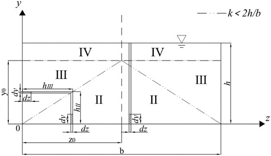
Figure 3.
Flow partition in a rectangular channel (k < 2h/b).
The flow velocity in Region IV is constant, due to which the flow velocity at any point is the mean velocity. Therefore, it is meaningless to find the depth of the average velocity point. In short, the depth of the average velocity point can be expressed using Equations (27)–(29).
2.3. Location of theCharacteristic Points in Different Regions
For Region I, measuring the velocity of points, in which the value of y equals h/e, can provide the mean velocity for the whole section in Region I. Therefore, the flow can be obtained by multiplying the mean velocity with the area. Similarly, the flow in Regions II, III and IV can be obtained using the same method. The differences between Region I and the others are as follows.
For Region IV, the velocity at each point inside the region is the mean velocity. For Regions II and III, all the LDAVs are connected in a line, as shown in Figure 4. Additionally, Figure 4 shows that PI, PII, and PIII are the characteristic points that represent the mean velocities in Regions I, II, and III, respectively.
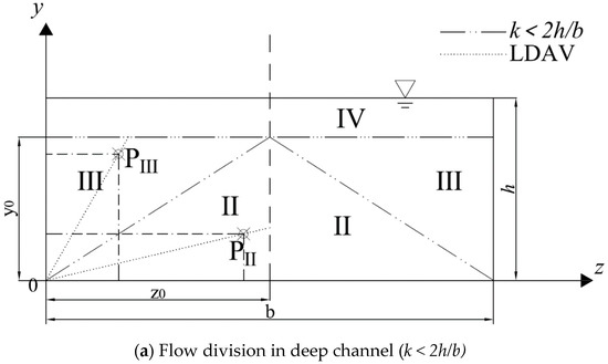
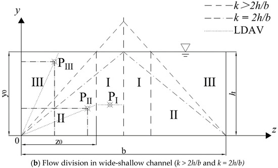
Figure 4.
Location map of the characteristic points and the line of depth average velocity (LDAV) in different flow partitions.
For Region II, the discharge Q can be expressed using Equation (30).
The mean velocity can be calculated from the value of Q/A, which can be expressed using Equation (31).
Combining Equation (11), Equation (14) and Equation (31) will produce Equation (32).
Therefore, the z value of the point, which can be used to calculate the value of Q of Region II, can be calculated using Equation (33).
The y value of the point can be expressed using Equation (34).
For Region III, it is similar to Region II. The value of z and value of y at the point, which can be used to calculate the value of Q of Region III, can be expressed using Equations (35) and (36).
3. Experimental and Results
3.1. Experimental Setup
The first experiment was conducted in a large-scale flow loop channel at the University of Wollongong (UOW), Australia (Figure 5). The channel was a rectangular open channel with a length, width and height of 11 m, 0.3 m and 0.45 m, respectively. Water was supplied to the channel from a constant head tank. The test section was located 6 m downstream of the inlet. The velocity was measured using a Dantec two-component LDA system. The equipment used in the experiment included a 60 mm fiber optic probe, a 400 mm focal length front lens, a 300mW continuous wave argon ion laser, and the transmit optics of the beam splitter Bragg cell and signal processor. In order to improve accuracy, particles were uniformly mixed into the fluid. In the experiment, the water depth was controlled by opening a baffle in the downstream tail water tank. When the required water depth was reached, the water depths upstream and downstream of the LDA installation position were measured, and the channel inlets had four positions at: X = 1.0 m, 2.6 m, 4.0 m and 6 m. When the water depths measured at these locations were equal, it was considered that the fluid in the rectangular open channel was uniformly flowing.
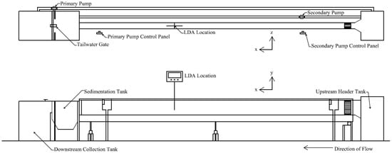
Figure 5.
Rectangular inclined water tank at the Fluid Mechanics Laboratory in the University of Wollongong (UOW), Australia.
The second experiment was carried out in a 6.3 m long, 0.8 m wide, 0.6 m deep rectangular inclined water tank at the Fluid Mechanics Laboratory of China Agricultural University (CAU), China, as shown in Figure 6. The main components of the channel were the head tank, the tail tank, the glass channel and the circular duct circulation system. The head tank was aligned with the center of the channel and was symmetrical with the center line of the glass water channel. Meanwhile, in order to make the flow velocity more uniform, a honeycomb steel plate was added at the entrance of the channel. An adjustable tail gate was installed at the end of the channel to change the water depth. Furthermore, Q was measured using an electromagnetic flowmeter installed on the inlet pipe. The flow velocity was measured using an acoustic doppler velocimetry (ADV). ADV is based on the principle of the acoustic doppler effect—the acoustic signal emits an ultrasonic signal from the probe, which is scattered by the particles in the water stream and then the scattered signal is received by the receiving probe. The ADV measures fluid velocity by comparing the Doppler phase shift of coherent acoustic pulses along three axes and transforming these to horizontal and vertical components.

Figure 6.
Schematic of the experimental device at China Agricultural University (CAU), China.
The experimental conditions were varied by adjusting the flow rate and flow depth.
3.2. Results
Equations (20) and (21) were verified by experimental data and the parameters of different experimental rectangular open channels are presented in Table 1. The experimental verification consisted of two parts. The experimental data for Run 1–Run 3 were obtained at the UOW, Australia, whereas those for Run 4–Run 11 were obtained at the CAU, China.

Table 1.
Summary of all the experimental conditions.
4. Discussion
The experimental data obtained at the UOW (Australia) and the theoretical locations of depth average velocity were compared, as shown in Figure 7, Figure 8 and Figure 9. The solid lines in Figure 7, Figure 8 and Figure 9 represent the locations of the depth average velocity calculated using Equations (20) and (21). The triangles represent the locations of the depth average velocity calculated using the interpolation of the experimental data. Figure 7, Figure 8 and Figure 9 show a significant consistency from the bottom corner to the middle of the channel. We also recognized that the theoretical locations of the depth average velocity calculated using Equations (20) and (21) can be used to determine the charge in the cross section of the rectangular channel.
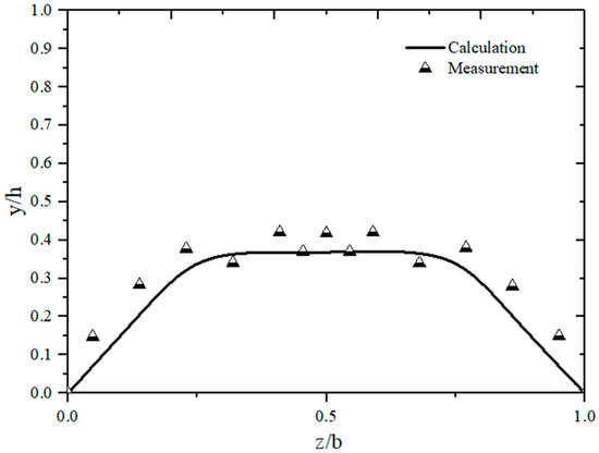
Figure 7.
Comparison of the location of depth average velocity between the calculated and measured values along different vertical lines from the bedform to the water surface (b/h = 4.615).
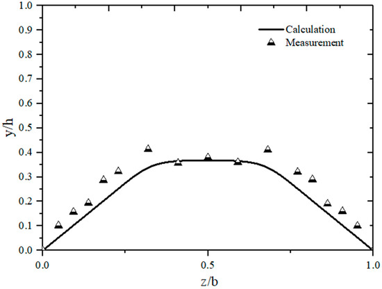
Figure 8.
Comparison of the location of depth average velocity between the calculated and measured values along different vertical lines from the bedform to the water surface (b/h = 3.297).

Figure 9.
Comparison of the location of depth average velocity between the calculated and measured values along different vertical lines from the bedform to the water surface (b/h = 2.727).
The values of b/h may have an effect on the empirical coefficient B in Equations (14) and (15), which may cause error between the calculated and measured values.
In order to demonstrate the performance of the location of depth average velocity (LDAV), the relative error between LDAV calculations (subscript l) and measurements (subscript i) is defined as: , where d refers to the depth average velocity along the same vertical lines from the bedform to the water surface under different water depths, as shown in Table 1. It should also be noted that LDAV relied on Log-Law, and the errors may be affected by secondary currents. According to the comparison, it is found that Equations (20) and (21) produced more realistic results both in Regions I and II, especially in the middle section of the channel. The relative differences of error between calculations and measurements increased from 11.9% to 13.8% as the aspect ratio decreased from 4.62 to 1.88. This further proved that this model is more suitable for use in a wide channel.
Through the experiments at the UOW, Australia, the location of the depth average velocity along the center line, as calculated by Equations (20) and (21), turns out to be highly consistent with the measurements. Therefore, in order to further verify the application of Equations (20) and (21) at the center line, a series of experiments concerning flow rate were conducted at different depths of the center line at the CAU, China. The results of experiments at the UOW and the CAU are shown in Figure 10.

Figure 10.
Velocity distribution and the location of depth average velocity in the center line under different experimental conditions ((a–f) show results for different aspect ratios).
5. Conclusions
In this paper, a laboratory study was conducted on the depth average velocity in a rectangular open channel. Based on the flow division theory and Log-Law, a correlation for calculating the location of depth average velocity on a vertical line from the bottom normal direction wall of different regions in an open rectangular channel is proposed. The main findings of this study are as follows.
- (1)
- The division lines cross above and on the water surface (Partition 1), whereas the location of depth average velocity can be calculated using Equation (20), Equation (21), and Equation (26) and the locations of the points which stand for the depth average velocity in different regions can be calculated using Equation (23), Equation (34), Equation (35) and Equation (36). According to the comparison between calculation and measurement, the current approach gives an average value of E, which is from 11.9% to 13.8%, thus proving the correctness of the flow division theory and the universality of the fitting correlation.
- (2)
- The division lines cross below the water surface (Partition 2), while the location of depth average velocity can be calculated using Equation (20), Equation (21), Equation (26), and Equation (29). It is found that the obtained results are consistent with the experimental measurements.
- (3)
- According to the comparison, it is found that the proposed correlation achieves an accurate matching both in Regions I and II, especially in the center line of the channel. It may be due to the fact that it is far from the side wall and is less affected by the shear stress of the side wall.
Therefore, the proposed correlation will simplify the procedure of vertical measuring profile measurements by only measuring the characteristic points representing the mean velocity of each region, and then, calculating the flow in different regions using the velocity-area method. It will be useful for flow measurement and the management of irrigation practices.
Author Contributions
Conceptualization, Y.H., J.C., and Z.M.; Methodology, Z.W., J.C., and Z.M.; Software, T.L., J.C., and Z.M.; Validation, Y.H., J.C., and Z.M.; Writing—Original Draft Preparation, Z.M., Z.W., and Y.H.; Project Administration, Y.H.; Funding Acquisition, Y.H., J.C., and L.Z.
Funding
The authors express gratitude for the financial support from the National Key R&D Program of China (Grant Nos. 2017YFC0403203, 2016YFC0400207, 2017YFD0701000 and 2016YFD200700). National Natural Science Foundation of China (Grant No. 51509248). Jilin Province Key R&D Plan Project (20180201036SF). Chinese Universities Scientific Fund (Grant Nos. 2019TC108, 10710301, 1071-31051012 and 1071-31051361). Open Fund of Synergistic Innovation Center of Jiangsu Modern Agricultural Equipment and Technology, Jiangsu University (Grant No. 4091600002). Open Fund of State Laboratory of Information Engineering in Surveying, Mapping and Remote Sensing, Wuhan University (Grant No. 19R06).
Acknowledgments
The authors are very grateful for the support of the fund.
Conflicts of Interest
The authors declare no conflict of interest.
References
- Cui, Y.; Wu, D.; Wang, S.; Wen, J.; Wang, H. Simulation and analysis of irrigation water consumption in multi-source water irrigation districts in Southern China based on modified SWAT model. Trans. Chin. Soc. Agric. Eng. 2018, 34, 94–100. [Google Scholar]
- Kitsikoudis, V.; Sidiropoulos, E.; Iliadis, L.; Hrissanthou, V. A machine learning approach for the mean flow velocity prediction in alluvial channels. Water Resour. Manag. 2015, 29, 4379–4395. [Google Scholar] [CrossRef]
- Han, Y.; Yang, S.Q.; Dharmasiri, N.; Sivakumar, M. Experimental study of smooth channel flow division based on velocity distribution. J. Hydraul. Eng. 2015, 141, 1–6. [Google Scholar] [CrossRef]
- Yang, S.Q.; Tan, S.K.; Lim, S.Y. Velocity distribution and dip-phenomenon in smooth uniform open channel flows. J. Hydraul. Eng. 2004, 130, 1179–1186. [Google Scholar] [CrossRef]
- Keulegan, G.H. Laws of turbulent flow in open channels. J. Res. Natl. Bur. Stand. 1938, 21, 707–741. [Google Scholar] [CrossRef]
- Coles, D. The Law of the wake in the turbulent boundary layer. J. Fluid Mech. 1956, 1, 191–226. [Google Scholar] [CrossRef]
- Nikuradse, J. Laws of flow in rough pipes. VDI-Forschungsheft 1950, 1933, 361. [Google Scholar]
- Hu, C.; Ni, J. Velocity distribution in smooth rectangular open channels. Hydro-Sci. Eng. 1988, 2, 19–2470. (In Chinese) [Google Scholar]
- Shiono, K.; Knight, D.W. Turbulent open-channel flows with variable depth across the channel. J. Fluid Mech. 1991, 222, 617–646. [Google Scholar] [CrossRef]
- Einstein, H.A.; EI-Samni, E.A. Hydrodynamic forces on a rough wall. Rev. Mod. Phys. 1949, 21, 520–524. [Google Scholar] [CrossRef]
- Chow, V.T. Open-Channel Hydraulics; McGraw-Hill Book Company: Singapore, 1973; pp. 32–46. [Google Scholar]
- Einstein, H.A. Formulas for the transportation of bed load. Trans. Am. Soc. Civ. Eng. 1942, 107, 561–597. [Google Scholar]
- Chien, N.; Wan, Z. Mechanics of Sediment Transport; ASCE Press: Reston, VA, USA, 1999; pp. 24–36. [Google Scholar]
- Daido, A. Effect of aspect ratio of channel and sediment density on transport phenomena. In Proceedings of the International Symposium on Hydraulic Research in Nature, Wuhan, China, 1992. [Google Scholar]
- Guo, J.; Julien, P. Shear stress in smooth rectangular open-channel flows. J. Hydraul. Eng.-Asce 2005, 131, 30–37. [Google Scholar] [CrossRef]
- Yang, S.Q. Interactions of Boundary Shear Stress, Velocity Distribution and Flow Resistance in 3-D Open Channels. Ph.D. Dissertation, Nanyang Technology University, Singapore, 1997. [Google Scholar]
- Yang, S.Q.; Han, Y.; Lin, P.Z.; Jiang, C.B.; Walker, R. Experimental study on the validity of flow region division. J. Hydro-Environ. Res. 2014, 8, 421–427. [Google Scholar] [CrossRef]
- Prandtl, L. Bericht uber untersuchungen zur ausgebildeten turbulenz. Zs Angew. Math. Mech. 1925, 5, 136–139. [Google Scholar] [CrossRef]


© 2019 by the authors. Licensee MDPI, Basel, Switzerland. This article is an open access article distributed under the terms and conditions of the Creative Commons Attribution (CC BY) license (http://creativecommons.org/licenses/by/4.0/).