Abstract
One question that often arises is whether a specialized code or a more general code may be equally suitable for fire modeling. This paper investigates the performance and capabilities of a specialized code (FDS) and a general-purpose code (FLUENT) to simulate a fire in the commercial area of an underground intermodal transportation station. In order to facilitate a more precise comparison between the two codes, especially with regard to ventilation issues, the number of factors that may affect the fire evolution is reduced by simplifying the scenario and the fire model. The codes are applied to the same fire scenario using a simplified fire model, which considers a source of mass, heat and species to characterize the fire focus, and whose results are also compared with those obtained using FDS and a combustion model. An oscillating behavior of the fire-induced convective heat and mass fluxes through the natural vents is predicted, whose frequency compares well with experimental results for the ranges of compartment heights and heat release rates considered. The results obtained with the two codes for the smoke and heat propagation patterns and convective fluxes through the forced and natural ventilation systems are discussed and compared to each other. The agreement is very good for the temperature and species concentration distributions and the overall flow pattern, whereas appreciable discrepancies are only found in the oscillatory behavior of the fire-induced convective heat and mass fluxes through the natural vents. The relative performance of the codes in terms of central processing unit (CPU) time consumption is also discussed.
1. Introduction
Performance-based design (PBD) principles are commonly used to draw up fire protection plans [1]. In light of the multiplicity of ventilation and fire-fighting systems that may be operational, both theoretical and empirical studies are frequently made (see, e.g., [2]). The results of the corresponding tests will help in drawing up protection, extinction and evacuation plans, perhaps even suggest improvements in the infrastructures themselves [3,4,5]. As may be expected, the main inconvenience of this approach is the expense involved in full-scale experiments.
Computational tools have contributed much to PBD in the case of confined areas such as stations, road tunnels, underground carparks shopping centres and stairwells of high-rise buildings [6,7,8,9,10]. Examples of reviews on field and zone approaches, turbulence, combustion, radiation, soot production and fire modeling in such scenarios can be found in [11,12].
However, despite the advances made in computational sciences, numerically modeling fires in buildings is still far from being an easy task because of the multiple combinations of scenarios and materials involved, the resulting chemical reactions, turbulent transport of smoke and heat, etc. As a consequence, numerical models are invariably simplified, although even such simplification still requires vast computational resources because the wide ranges of scales involved and the multi-dimensional and unsteady nature of the problem cannot be avoided when analyzing complex real scenarios.
To simulate compartment fires, the computational codes used include Fire Dynamics Simulator (FDS), FireFOAM, OpenFOAM, PHOENICS, FLUENT and CFX, among others (see, e.g., [7,10,12,13,14,15,16,17]). All these codes have been extensively validated for a great variety of fire scenarios in the case of the first two and for a very large number of applications in the field of fluid mechanics in the case of the others. Despite the exhaustive validation of the codes, the uncertainties involved in experimental studies of complex large-scale fires (associated with data collection and the specification of the fire scenario and detailed experimental conditions), the variety of simplifications introduced in the governing equations for modeling turbulent transport and combustion processes, and the multiplicity of possible scenarios where a fire can occur, among other factors, introduce uncertainty in the assessment of the relative merits of different simulation tools, whether specialized or general-purpose.
In this work we compare the performance and capabilities of a specialized code (FDS) [18,19], which is a code specifically designed for low-speed fire-driven flows, developed by the National Institute of Standards and Technology (NIST), and a general-purpose code (FLUENT) [20] for the numerical simulation of a fire in the commercial area of an underground intermodal transportation station. Details on the verification and validation of FDS can be found, respectively, in Volumes 2 and 3 of the FDS Technical Reference Guide [21,22]. Both codes, which are among the most frequently used in the literature to analyze, respectively, fire-related and general thermo-fluid dynamics problems, have been thoroughly validated against experimental results (see, e.g., [23,24,25]). However, the above mentioned uncertainties involved in large-scale tests, along with difficulties in obtaining well resolved solutions because of practical computer limitations and inappropriate specification of the numerical and boundary conditions settings, make it often difficult to assess the accuracy and efficiency of the codes used to simulate a fire in a particular complex facility. Furthermore, fires can involve a wide variety of scenarios, with different possible burning materials, which represents a huge challenge for simulation programs. Precisely for this reason, and in order to make a more general comparison between the codes considered, less dependent on specific sub-models, and more particularly focused on the oscillatory behavior of the flow through openings, we have tried to simplify as much as possible some aspects that determine the evolution of the fire. To this end, the scenario and the fire model are simplified by reducing the number of factors that may affect the fire evolution. More specifically, a simplified fire model, which considers a source of mass, heat and species to characterize the fire focus, is used. In order to investigate whether the simplified model can reproduce the essential aspects of the fire, it has been first validated with a combustion model using the FDS code. Then, the results for the smoke and heat propagation patterns and convective heat and mass fluxes through the natural vents, obtained with the two codes using the simplified fire model, are compared and discussed in detail. The predicted oscillating behavior of the fire-induced convective fluxes through the open vents is compared with experimental results obtained by other authors. The CPU times consumed by the two fire models and codes are also compared.
2. Numerical Models
The mass, momentum and internal energy conservation equations, along with appropriate turbulence and fire models, are solved using the FDS (v. 6.1.2) and FLUENT (v. 6.3.26) codes, which use finite-differences and finite-volume discretization schemes, respectively, and are second-order accurate. Details on the discretization schemes can be found in [19,20].
2.1. Turbulence Model
In a previous work [26] we compared the results obtained using LES (Large Eddy Simulation) and RANS (Reynolds Averaged Navier Stokes equations) models for a scenario similar to that considered here, showing the advantage of using LES. Therefore, all the results of the present work were obtained using LES to simulate turbulence. In FDS, the Deardorff eddy viscosity subgrid-scale (SGS) model [27] (default choice in version 6.1.2 of the code) was used in most of the simulations. In this model, the turbulent viscosity is expressed as , where , the filter width and is the subgrid-scale kinetic energy [18,19]. The turbulent Schmidt and Prandtl numbers are set equal to the default value of 0.5, although the effects of using other values will also be investigated. The influence of different SGS models on the numerical results was assessed by using, as an alternative, the Smagorinsky model with different values of the model constant [18,19]. In FLUENT, we used a LES model with the default options (Smagorinsky-Lilly SGS model, with ).
2.2. Combustion Model
One aspect that can substantially and in many ways determine the evolution of a fire is the type of burning material. Bearing in mind that it is not the purpose of this paper to focus attention on complex combustion and soot formation processes, and despite the fact that fires in public spaces will inevitably involve many different materials, we consider heptane as the burning fuel, as it has been in other fire simulation studies (see, e.g., [7,25,28]). Although the combustion of this substance involves a large number of chemical reactions and species, we only consider the production and transport of those resulting from the reaction . Other products such as and soot have not been considered, although the transport of other species (except, for example, soot, which would require a more complex treatment) could also be easily handled. Not considering soot production is an additional simplification in the fire model aimed at minimizing the differences between the FDS and FLUENT settings, so that the comparison between the results of the two codes can focus primarily on aspects such as those related to the oscillatory flow through open vents.
One of the two fire models considered in this work is the EDC (Eddy Dissipation Concept) non-premixed combustion model implemented by default in version 6.1.2 of FDS [18,29], based on the infinitely fast, mixing-limited reaction approximation, in which fuel is locally consumed at a rate which is proportional to both the mixing rate and the limiting concentration of reactant, and the production rates of species mass times the respective heats of formation are summed to determine the heat release per unit volume. The model for the mixing time scale is discussed in [29].
2.3. Simplified Fire Model
As an alternative to the EDC combustion model, we have modeled the fire by directly introducing the gases generated from combustion, at temperature , through an inlet section of area , with a mass flow rate .
The combustion products constitute a mixture that is assumed to behave as a conserved scalar, whose properties (viscosity, thermal conductivity, mass diffusivity and molecular weight) are the average of those of its constituent species. The distributions of mass fractions of species are determined from the conserved scalar concentration and mass fractions , , and at the fire focus. For a different composition of the combustion gases, the transport of CO and other species could be carried out in a similar way. Thus, the problem would be reduced to knowing the amount of CO and other species produced at the fire focus, which, in turn, would depend on the type of material burned and the ventilation conditions. As indicated above, in order to be realistic, the complex analysis of the influence of different types of burning materials on the evolution of the fire has been left outside the scope of this work.
In the simulations involving both FDS and FLUENT the temperature dependency of the specific heats of carbon dioxide, water vapor and nitrogen, , was expressed by a 4th order polynomial function and, in the case of air, by a 7th order polynomial function . This is the default option in FDS. The data in the FLUENT and FDS databases are very similar, although the default option in the former is to set the specific heat of any species as constant. The molecular weight, , and specific heat, , of the mixture are calculated as
where is the number of species and the molar fraction of species i.
The rate of heat convected through the inlet section is calculated as
where the ambient temperature, , is set equal to the reference temperature , and . Here, is the density and the velocity of the mixture of gases at the inlet section ( is the ambient pressure). It is assumed that the temperature, density, velocity and composition of the gas entering the domain are time-independent and uniform across the inlet section. Note that, once heat release rate () and are fixed, the choice of determines and, thus, the mass flow rate, . One of the goals of this paper is to determine whether the effects of turbulent mixing and flame radiation on fire evolution, in regions near or far from the fire focus, are well reproduced for different combinations of and values.
2.4. Radiation Model
FDS uses techniques for radiative transport similar to those used in finite volume methods for convective transport in fluid flow [30]. When using the combustion model, the fraction of the energy released in the fire that is emitted as thermal radiation may be specified as a source term in the radiation transport equation through parameter RADIATIVE FRACTION, or calculated by the radiation model implemented in FDS [19] by setting . We have tested both options, with a specified fraction of the HRR emitted as thermal radiation of in the first case, and the results obtained did not differ significantly. Therefore, only the results obtained with the second option will be shown below. In FLUENT, the default P1 radiation model was used [20]. The actual amount of radiation absorbed or emitted by the hot gases in the simulations we run, which depended on the local mass fractions of the gas mixture considered and the properties of each gas, is expected to be lower than that obtained if the production of soot were taken into account.
3. Fire Scenario
3.1. Description of the Facility
In a previous contribution we studied the bus maneuvering and parking zones of the underground transportation hub “Avenida de América”, in Madrid, Spain. Here, we focus on a fire that starts in a commercial premises (one of twenty) situated on level −3 (Figure 1a). The different levels are connected by escalators. The computational domain considered in all the simulations, shown in Figure 1b, only includes the commercial area at level −3. The overall dimensions of the zone studied are 66.66 × 39.86 m, with a usable floor area of 2085 m2. In the geometric models created in FDS and FLUENT, the x and y axes are horizontal, and the z axis is vertical. The origin of the coordinate system is located in the S-W corner of the commercial area. It is assumed that the floor and ceiling surfaces are flat and horizontal and that the height is uniformly 3 m. As mentioned above, the origin of the fire is a commercial premises in the N-W corner of the shopping area. The danger is greater at this site because of the proximity to the stairs and consequent risk of spreading vertically and because of the greater affluence of people, which would hinder evacuation. There are two escalators connecting level −3 with level −2, and 11 1200 × 600 mm air extraction grilles installed in the ceiling, which form part of the forced ventilation system.
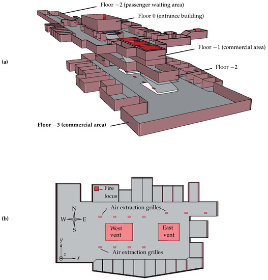
Figure 1.
(a) Schematic view of the transportation station building (excluding platforms). (b) Top view of the shopping area where the fire originates (level −3): natural and forced ventilation systems, fire focus and reference system.
In a previous work [26], upper levels of the station (Figure 1a) were included in the computational domain in order to study the smoke and heat propagated not only in the commercial area at level −3, but also in the stairwell that connects levels from −3 to 0 and through the natural ventilation outlets installed at the ceiling of level −1. The evolution of the fire throughout level −3 when the upper levels were included and when the stairwells of level −3 were assumed to be open to the atmosphere did not show significant variations. Therefore, in order to better focus on the fire spread through level −3 only, where the most relevant effects were observed, we will assume that the commercial area is directly open to the atmosphere through two outlet sections (see Figure 1b), located 70 cm above the ceiling of level −3, with the same areas of 81.37 m2 (west vent) and 60.06 m2 (east vent) as the horizontal pass-through sections of the stairwells located on the W and E sides, respectively. As the aim of the present work is to analyze the evolution of the fire using different codes and fire models rather than evaluating the effectiveness of particular measures to limit the spread of the fire to the top floors of the building, no smoke barriers were included around the outlets. Note that, since there are not any additional natural vents or other means for introducing fresh air from outside, the necessary makeup air will inevitably be drawn through one or both existing vents, as will be shown below.
3.2. Boundary Conditions
Boundary conditions at the fire focus are applied on a square floor surface area () of the premises where the fire focus is located. In most of the simulations presented in this work a total heat release rate = 2.5 MW is assumed, which lays in the range of typical HRR values (270 to 1200 kWm−2) for fires that may occur in shops [31]. When using both the simplified fire model and the EDC combustion model, we assumed that the indicated HRR value (or the mean value around which HRR oscillates in the combustion model) is reached almost instantaneously. Although we could have used a more realistic curve to describe the evolution of HRR, this simplification will facilitate the comparison between codes (while avoiding the introduction of additional parameters) and will not hinder the study of the oscillatory flow through the ceiling vents, a process that is usually settled long before the fire starts to decay, at least for fire scenarios similar to that explored in this paper.
When the combustion model is used, we assume that the burning fuel is heptane, with a heat of combustion = 44.566 MJ kg−1 [32]. The default values for all other chemical and physical properties set by the FDS code are assumed. The heptane evaporation speed and fuel burning rate will not be a part of the solution; instead, the above mentioned HRR value is imposed. As mentioned before, the parameter RADIATIVE FRACTION is set equal to 0.
In the case of the simplified fire model (Section 2.3), inflow boundary conditions are applied at the inlet section of the fire focus. A mixture of gases with the composition indicated in Section 2.3 enters the domain with a mass flow rate , at temperature and velocity , yielding a convective HRR of 2.5 MW. The emissivity of the inlet surface is set to 0 to avoid any additional contribution to the heat release rate due to thermal radiation.
To keep the thermal boundary conditions as similar as possible for both the combustion and simplified fire models, zero emissivity and a very small liquid conductivity value at the heptane free surface are imposed.
To select a suitable value for , the area to which the fire is expected to spread should be taken into account. A suitable value of the inlet velocity must also be selected to ensure a realistic ratio between inertial and buoyancy effects [33]. However, such parameters are expected to be less important the further one moves away from the focus of the fire, although their values must be chosen so that the dimensionless HRR (source Froude number [33]) remains representative of buoyant fires:
where subscript a denotes ambient value, is the specific heat of air, g is the gravity acceleration and is an equivalent fire focus diameter. In all the simulations we will assume an area of the fire focus inlet section = 3 m2, for which the above data provide a value of around 0.42 for , which is within the range considered normal for buoyant fires [33].
Table 1 shows the details of the four different combinations (labeled as cases G-1 to G-4) of and , which yield a convective HRR of 2.5 MW. The temperature range considered is intended to include the typical average temperatures of the combustion products. The mass flow rate of carbon dioxide is .

Table 1.
Conditions simulated with the simplified fire model (cases G-1 to G-4), run with Fire Dynamics Simulator (FDS) and FLUENT.
In order to reproduce approximately the real operating conditions of the facility, we assume that the air flow rate extracted through the forced ventilation system on level-3 is constant from the outset of the fire (40,000 m3 h−1) and uniformly distributed among all the extraction grilles, assuming that the fire does not affect the operation of the extraction units. The indicated value approximately corresponds to a number of 6 to 7 air changes per hour, which is in accordance with the Spanish regulations [34].
At the west and east natural vents, which are both assumed to be open during the simulations, the gauge pressure is set to 0, a condition which is imposed through OPEN and PRESSURE OUTLET boundary conditions in FDS and FLUENT codes, respectively. Details about the implementation of the two types of boundary conditions, which are essentially the same, can be found in [19,20]. The results obtained with FDS were very sensitive to the inadequate implementation of the inflow and outflow boundary conditions, especially when a grid partition exists in the area closed to the fire focus and the open vents, and so special care was taken to avoid these situations.
At all the walls, zero heat flux and no-slip boundary conditions are applied, without modeling the conjugate heat transfer problem. Although the assumption of adiabatic walls might not be considered sufficiently realistic, such an assumption allows us to reduce the number of factors to be considered that affect the fire evolution, and thus to carry out a more precise comparison between FDS and FLUENT performance in the prediction of the basic thermo-fluid dynamic aspects that determine the fire evolution.
3.3. Computational Grid
Four different hexahedral computational grids of about 1017 k, 3358 k, 7074 k and 19,864 k cells were used to run the simulations. The grid adaptation capabilities of FLUENT, which facilitate the meshing of complex geometries and local refinement, were not used so that the grid characteristics would be similar when comparing FDS. A uniform cell size in all directions was used for all grids in the region , whereas a grid refinement in z direction was applied in the vicinity of the ceiling () in order to better resolve the flow near the wall. To choose an appropriate order of magnitude for the size of the grid cells, the range of scales that must be resolved to obtain an acceptable accuracy in the results was determined following the criterion that the estimated characteristic length of the fire plume [35],
should be spanned by at least ten computational cells [28]. For the general scenario conditions described above ( = 2.5 MW, = 1.17 kg m−3, = 1011 J kg−1 K−1 and = 300 K), we obtain . In the region , the cell size in z direction, , gradually shrinks to at the ceiling () in order to ensure suitable values of the parameter . Table 2 shows, for each computational grid, the total number of cells, the approximate cell size in the region , , the approximate number of grid cells, , spanning the characteristic length L, and the grid size in z direction at the ceiling, .
Table 2.
Grid characteristics: total number of cells, approximate cell size (), approximate number of cells () spanning the characteristic length L, and grid size () in z direction at the ceiling ().
Most of the results presented in the following section were obtained using grid II (), whereas grids I (coarsest), III and IV (finest) were used for testing grid independence.
FDS uses an explicit scheme in time, and automatically adjusts the time step required for numerical stability during the simulation, so that the following condition is met:
The default maximum and minimum CFL numbers used by FDS are, respectively, 1 and 0.8. Mean values of and 1.8 ms were obtained from Equation (5) when using the simplified fire model and the EDC combustion model, respectively.
On the other hand, a fully-implicit scheme was used for time advancement in FLUENT, and no stability criterion was taken into account to calculate . Instead, we used a constant time step during the simulations. All residuals diminished by at least two orders of magnitude after around 40 to 50 iterations per time step, and then remained almost constant. The scaled residuals defined in FLUENT [20] for the mass, species, three components of momentum, and energy and radiation equations decreased to around , , and , respectively.
It should be pointed out that, for the same scenario and equivalent simulation settings, FLUENT is considerably more time consuming than FDS, and obtaining strictly time step-independent solutions may require substantially higher CPU times. In fact, reducing the time step used with FLUENT to obtain the results presented in the next section would still produce small changes in the results, although not be very significant for the purposes of comparison with FDS.
4. Results and Discussion
This section looks at the results obtained from the simulation of the scenario described in Section 3.2 using the FDS and FLUENT codes with the simplified fire model and the default EDC combustion model implemented in FDS. The results obtained are the temperature and concentration contours in horizontal and vertical sections of the domain, heat flow rates and mass flow rates extracted from the ventilation systems, and mass flow rates leaving and entering the compartment through the ceiling vents.
First, we discuss the sensitivity of the results obtained with FDS to the grid size and different settings of the LES turbulence model. Then, we analyze the predictions of FDS with the simplified fire model, considering four combinations of the inlet temperature, , and mass flow rate, , of the mixture of gases introduced in the computational domain (cases G-1 to G-4 of Table 1). The results obtained for the oscillatory flow through vents are compared with experimental results available in the literature. Then, we compare the results for the fire evolution obtained with the simplified fire model (Case G-1 of Table 1) and the EDC combustion model (with ) using the FDS code. Finally, the results obtained with the simplified fire model using the FDS and FLUENT codes are compared to each other.
Except in Section 4.1, the respective default settings for the LES model were used in each code, and a computational grid with was used in all the simulations described below.
4.1. Preliminary Tests
Several tests were carried out to investigate the grid independence of the FDS results using the four computational grids of Table 2. Using the simplified fire model with (Case G-4 in Table 1), results for mass flow rate extracted by the ventilation systems, shown in Figure 2a, can be considered fairly grid independent even for the relatively coarse grid II, as well as results for heat flow rate and temperature and mass fraction contours on vertical and horizontal sections of the domain (not shown here).
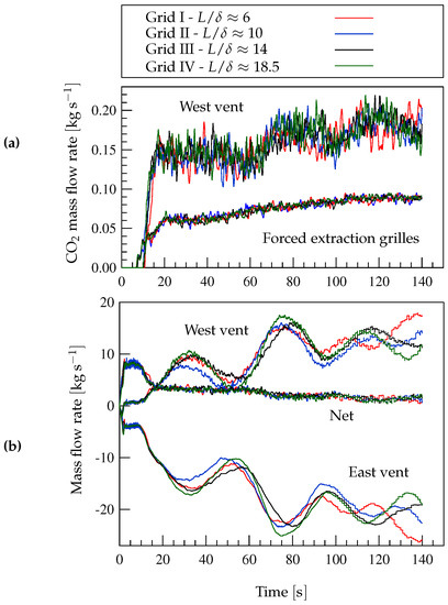
Figure 2.
(a) Mass flow rates of through the ventilation systems and (b) mass flow rates through the west and east vents (positive outwards) and net mass flow rate leaving the compartment, obtained with FDS, the simplified fire model with (Case G-4 in Table 1) and grids with and .
Figure 2b shows the mass flow rate (positive outwards) through the west and east natural vents and the net mass flow rate leaving the compartment.
The results depicted in Figure 2b show an acceptable degree of grid independence for grids II and finer, especially in terms of the net mass flow rate. However, note that the oscillating mass flow rates through the open vents are very sensitive to the grid size, and differences remain between the results obtained with grids III and IV. Indeed, the dependence of these unsteady results on grid size could not be completely avoided unless an extremely fine grid were used. However, the temperature and mass fraction contours, the heat and mass flow rates through the forced and natural ventilation systems (Figure 2a) and the net mass flow rate leaving the compartment (Figure 2b) do not appreciably change when using grids with or , and, therefore, the computational grid with (grid II) can be considered sufficiently fine to reach grid independency for the most relevant results. As for the FLUENT code, it was shown in [26] that, for the current scenario, a grid with is also fine enough to reach grid independency for the most relevant results. However, the comparison between Figure 2a and the equivalent results shown in [26] shows that FLUENT, when using LES, is more sensitive to the grid size than FDS in predicting, for example, the mass flow rate through the forced extraction grilles.
The Deardorff and Smagorinsky SGS models are the default options for LES models in FDS and FLUENT, respectively [19,20]. We ran simulations with FDS, using both SGS models, two values for the coefficient of the Smagorinsky model ( and , the latter being the default value in FLUENT) and two combinations for the turbulent Prandtl and Schmidt numbers ( and , which are the default values in FDS and FLUENT, respectively). As in the grid independence test, the results obtained for the mass flow rates through the west and east vents (not shown here) appear to be the most sensitive ones to the settings used for the SGS model (differences for other quantities such as the mass flow rate through the forced extraction grilles and net mass flow rate leaving the compartment are much smaller). Moreover, differences are significant only between the results obtained with FDS and FLUENT, whereas using different settings for the SGS model in FDS does not affect the results substantially.
4.2. Results of the Simplified Fire Model
Figure 3 shows the results for the heat flow rate through the ventilation systems, obtained with FDS using the simplified fire model with the four combinations of and of cases G-1 to G-4 (Table 1).
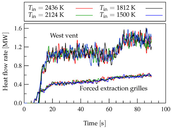
Figure 3.
Heat flow rate through the forced extraction grilles and west vent, predicted by FDS and the simplified fire model with and (cases G-1 to G-4 in Table 1).
Note that, despite the broad range of inlet temperatures considered (2436–1500 K), maintaining the same convective heat release rate (calculated from Equation (2)) in all the cases yields results that compare very well with each other. The results for the normalized mass flow rate (, where is the mass flow rate of introduced in the domain at the fire focus) are qualitatively very similar to those for the heat flow rate shown in Figure 3. Although not shown here, the results for the mass flow rate extracted by the forced ventilation system and net mass flow rate leaving the compartment are practically independent of .
Table 3 shows the fractions of the heat and mass introduced in the domain from the beginning of the fire that had been extracted by the ventilation systems at and ,
Table 3.
Fractions (in %) of heat () and mass of () extracted by the natural and forced ventilation systems (Equation (6)). In parentheses, variation (in %) with respect to Case G-1. Values obtained with FDS and the simplified fire model after the first (cases G-1 to G-4) and (cases G-1 and G-4) of the fire.
Note the low dependence of and on the inlet temperature .
Figure 4 shows the temperature contours at on horizontal planes at heights and , and at and , predicted by FDS using the simplified fire model with and . It can be observed that, sufficiently far from the fire focus, the temperature distributions obtained using different values compare very well, behavior that is consistent with the very slight dependence of the results of Figure 3 and Table 3 on . A similar behavior is observed for the distributions of the normalized concentration and velocity magnitude, which are not shown for brevity.
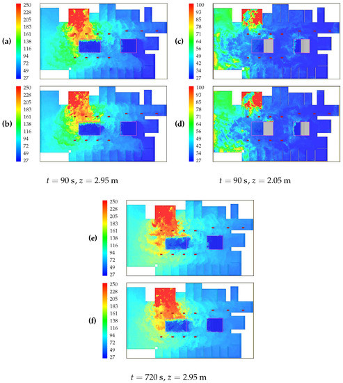
Figure 4.
Temperature contours () at instant and and (top pictures), and at and (bottom pictures). Results obtained with FDS, a grid with and the simplified fire model with (a) , (b) , (c) , (d) , (e) and (f) (cases G-1 and G-4 in Table 1).
4.2.1. Oscillatory Flow through Ceiling Vents
Figure 5a shows, for Case G-4 (), the FDS results for the mass flow rates leaving and entering the compartment through the west vent ( and , respectively), the net mass flow rate through this vent () and the mass flow rate entering the compartment through the east vent (). During the whole simulation, the outward mass flow rate through the east vent is negligible compared to the inward one. On the other hand, hot gases flow outward through the north side of the west vent (closer to the fire focus; see Figure 1b) and cool air at ambient conditions () flows inward through the south side. The bidirectional flow predicted through the west vent is widely described in the literature (see, for example, [36,37,38]). In the problem considered, whether the flow across the vents is induced by buoyancy or by a fire-generated pressure difference is determined by the Richardson number, which can be expressed as [38,39]
where Gr and Re are the Grashof and Reynolds numbers, D is the vent size, is the variation of density across the vent and is the pressure increment due to thermal expansion, calculated as
where and are the density and temperature in the vicinity of the vent, is a discharge coefficient and A is the area of the vent. In the scenario of Figure 5a, using the mean values of density and temperature obtained from the simulation at s over the west vent (of area ) yields , and , a value indicating that the flow is dominated by buoyancy. As the mean temperature around the vent increases, reaches values above for .
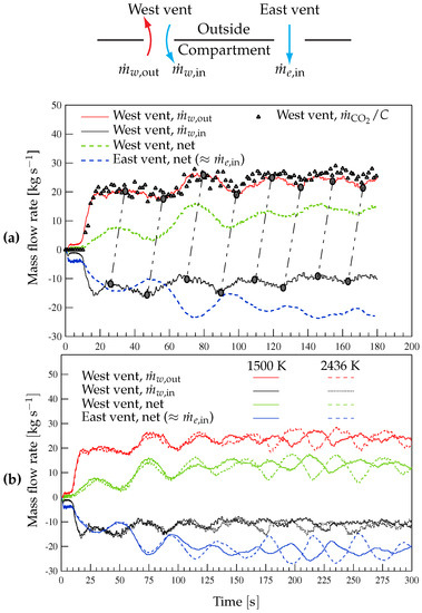
Figure 5.
(a) Mass flow rates through the west and east vents obtained with FDS for Case G-4 (). Triangle symbols: mass flow rate through the west vent divided by . (b) Comparison between FDS results for the mass flow rates through the west and east vents for cases G-1 and G-4 ( and ).
It can be observed from Figure 5a that the inward and outward mass flow rates across the west vent oscillate. Note that the outward mass flow rate oscillation wave has a slight and approximately constant delay of about with respect to the inward flow wave. Also note that the resulting oscillating net mass flow rate across the west vent determines the oscillating behavior of the inward flow through the east vent, with the same frequency (of about , calculated over a simulation of ) and approximately the same wave shape and time-dependent amplitude. This behavior was observed for all the simulations run.
Figure 5a also shows the results for the evolution of the mass flow rate through the west vent divided by the constant (triangle symbols). The approximate coincidence between these results and the outward mass flow rate through the west vent means that the concentration of in the hot gases leaving the compartment is fairly constant, and varies from approximately during the first two minutes after the instant at which the gases begin to flow (around ) to once the simulation reaches a steady state.
Figure 5b compares the results of Figure 5a, for , with those obtained with . Note that the frequency of the mass flow rate oscillations is only slightly smaller and their amplitude remains more constant with time for the higher value. The absolute values of the net mass flow rates across the west and east vents obtained with both values are in phase to each other and oscillate with very similar amplitudes. Also note that the mentioned delay of about between the outward and inward mass flow rate oscillation waves also exists in the results obtained with . Therefore, the influence of on the overall oscillatory behavior of the flow at the open vents is apparently small.
4.2.2. Comparison with Experiments
The dependence of the frequency of the oscillating flow through the open vents was found to be well described by expressions of the form
(see [37] and references therein for a review of results available in the literature). From experimental and numerical results it was shown in [40,41] that the flow oscillation frequency in a compartment fire with two open vents is proportional to . A similar problem but for a compartment with a single horizontal ceiling vent was studied numerically in [42], where the flow oscillation frequency was found to be proportional to for heat release rates below a critical value. Figure 6a shows the numerical results for the oscillation frequency as a function of the heat release rate (in the interval 500 to ) obtained in the present work using FDS and the simplified fire model, with and . The figure also shows the correlation
which fits the FDS results with , along with correlations of the form of Equation (7), with the values of the exponent n proposed in [40,41,42]. Note that the results for the oscillation frequency obtained in the present work exhibit a dependence on the HRR that is very close to that of the experimental results of [40,41].
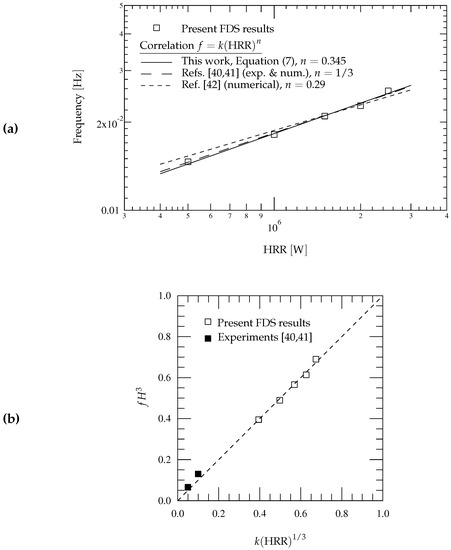
Figure 6.
(a) Oscillation frequency of the fire-induced flow through the open vents as a function of heat release rate (HRR). Comparison of the present numerical results with correlations of the form of Equation (7) with values of the exponent n deduced from experimental and numerical results [40,41,42]. (b) Collapse of FDS and experimental results on the correlation with .
Figure 6b shows a comparison between the present numerical results and the experimental results of [40,41], obtained in a cubic enclosure of side m for thermal powers of 1 and , for which the measured frequencies were and , respectively. Although the experimental results available for comparison are scarce, it is interesting to point out that numerical and experimental results collapse very well after scaling on the curve , despite the wide ranges of the compartment height, H, and HRR values considered.
4.3. Combustion Model vs. Simplified Fire Models
Figure 7 shows the HRR as a function of time in FDS simulations that use the simplified fire model (cases G-1 to G-4) and the EDC combustion model. In the first case, the energy enters the domain at a constant rate, whereas in the second one the HRR exhibits high frequency fluctuations, with an amplitude that approximately varies in the range 1.0 to . As will be shown below, these fluctuations produce high-frequency fluctuations of small amplitude in the heat and mass flow rates through the ventilation systems, especially through the west vent.
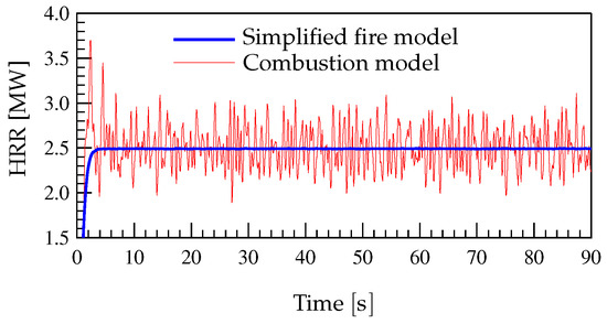
Figure 7.
Heat release rate (HRR) in the simulations of cases G-1 to G-4 (Table 1), compared with that of the EDC combustion model.
Figure 8 shows the temperature and mass fraction contours at instant and vertical planes at and , obtained with the combustion model and the simplified fire model (Case G-1). Figure 9 shows the temperature and velocity magnitude contours at , on the horizontal plane at , obtained with FDS using the EDC combustion model and the simplified fire model (Case G-1). Figure 10 shows the mass fraction contours at , on the horizontal planes at (left column) and (right column), obtained as in Figure 9. It can be observed from the figures the very good overall agreement between the three types of results obtained with the combustion and simplified models.
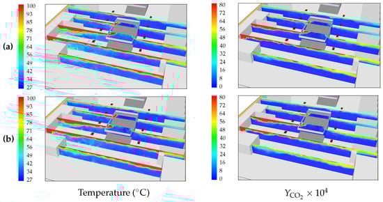
Figure 8.
Temperature contours () (left column) and mass fraction contours () (right column) at instant and and , obtained with FDS using a grid with . (a) Combustion model with and (b) simplified fire model with (Case G-1).
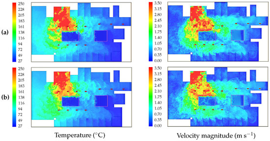
Figure 9.
Temperature contours (left column) and velocity magnitude contours (right column) at , on the horizontal plane at , obtained as in Figure 8. (a) Combustion model with and (b) simplified fire model with (Case G-1).
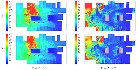
Figure 10.
Contours of mass fraction () at and heights (left column) and (right column), obtained as in Figure 8. (a) Combustion model with and (b) simplified fire model with (Case G-1).
Figure 11 shows the results for the mass of and heat flow rates through the ventilation systems obtained with FDS using the simplified fire model (Case G-1) and the combustion model. Note that the combustion model predicts mass of flow rates through the forced ventilation grilles slightly larger than those obtained with the simplified fire model, a behavior that could be explained by the higher concentrations at the ceiling in the vicinity of the forced extraction grilles, as shown in Figure 10. Also note the very good degree of agreement between the results for the flow rates through the west vent obtained with FDS and the two fire models. This can be seen with more detail in Figure 12, which compares results similar to those presented in Figure 5b, obtained with FDS using the combustion model and the simplified fire model. Note that the outward mass flow rate through the west vent predicted with the combustion model oscillates with a slightly smaller amplitude than when using the simplified fire model, an effect that is also observed in the net mass flow rate through the west vent and, as a consequence, in the inward mass flow rate through the east vent.
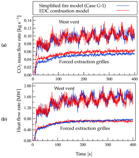
Figure 11.
(a) Mass flow rates of , and (b) heat flow rates through the ventilation systems, obtained with FDS as in Figure 8.
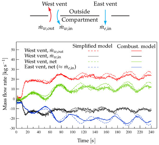
Table 4 shows the relative CPU time consumed by FDS using the EDC combustion model and the simplified fire model. Note that the combustion model consumes a CPU time around 40% larger than that consumed when the simplified fire model is used, with no appreciable change in the results, as shown above. Using the default value of instead of zero for the parameter RADIATIVE FRACTION reduces the CPU time consumed by the combustion model by about 7%, with very little difference in the overall results.
Table 4.
CPU time (relative to Case G-1) in FDS simulations.
4.4. FDS vs. FLUENT
Figure 13, Figure 14, Figure 15, Figure 16, Figure 17 and Figure 18 show comparisons between temperature, velocity magnitude and mass fraction contours obtained with FDS and FLUENT at several vertical and horizontal planes and two different instants. It can be observed from the figures that the overall degree of agreement is very good. The most noticeable differences between FDS and FLUENT results are systematically observed in the distribution of the concentration in the vicinity of the ceiling, as can be observed from Figure 17 and Figure 18, and pictures at the right column of Figure 13 and Figure 14.
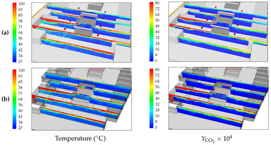
Figure 13.
Temperature contours () (left column) and mass fraction contours () (right column) at instant and and obtained using a grid with , the simplified fire model with (Case G-1) and (a) FDS and (b) FLUENT codes.
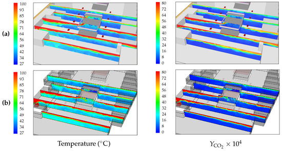
Figure 14.
Temperature contours () (left column) and mass fraction contours () (right column) at instant and and , obtained as in Figure 13. (a) FDS; (b) FLUENT.
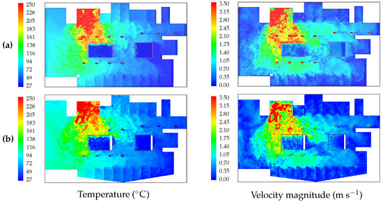
Figure 15.
Temperature contours (left column) and velocity magnitude contours (right column) at , on the horizontal plane at , obtained as in Figure 13. (a) FDS; (b) FLUENT.
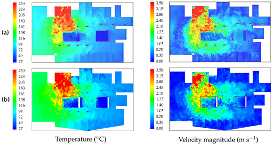
Figure 16.
Temperature contours (left column) and velocity magnitude contours (right column) at , obtained as in Figure 13. (a) FDS; (b) FLUENT.
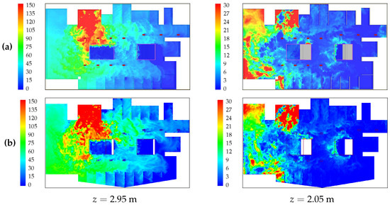
Figure 17.
Contours of mass fraction () at and heights (left column) and (right column), obtained as in Figure 13. (a) FDS; (b) FLUENT.
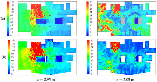
Figure 18.
Contours of mass fraction () at and heights (left column) and (right column), obtained as in Figure 13. (a) FDS; (b) FLUENT.
As in previous sections, the most sensitive results to the use of FDS or FLUENT codes are related to the flow rates through the ventilation systems, and, therefore, we will discuss in the following the main differences found in the results for these quantities when using the two codes. Figure 19a,b compare the results obtained with FDS and FLUENT for the evolution of the mass and heat flow rates, respectively, through the open vents and forced extraction grilles, using the simplified fire model with (Case G-4). The degree of agreement between the FDS and FLUENT results is very good, especially for the heat flow rates. Note that FLUENT predicts values for the mass flow rates extracted through the forced extraction grilles and through the west vent that are higher and lower, respectively, than those predicted by FDS, which can be attributed to the higher concentrations at the ceiling in the vicinity of the forced extraction grilles, as shown in Figure 17 and Figure 18. However, despite the differences in the values predicted by FLUENT and FDS for the mass of extracted over through the forced (83.27 vs. 73.20 kg) and natural (134.5 vs. 143.6 kg) ventilation systems, the difference in the total mass extracted over that time period is less than . The reasons for these relatively low discrepancies are not completely clear. Note that the higher Schmidt number used by default in FLUENT would produce a lower diffusion and therefore a higher concentration near the ceiling, resulting in a higher mass flow rate through the forced ventilation grilles and a lower extraction rate through the west vent. Also note that the slightly lower outward mass flow rate through the west vent predicted by FLUENT, as will be shown below, may also contribute to explain the differences.
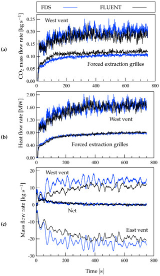
Figure 19.
(a) Mass flow rates of , (b) heat flow rates, and (c) mass flow rates (including the net mass flow rate leaving the compartment) through the ventilation systems obtained with FDS and FLUENT using the simplified fire model with (Case G-4).
Figure 19c compares the FDS and FLUENT results for the net mass flow rates through the west and east vents, and the net mass flow rate leaving the compartment, obtained with the simplified fire model with (Case G-4). The agreement between both types of results for the net mass flow rate leaving the compartment is very good. Note that approximately 12 minutes after the beginning of the fire the net mass flow rate leaving the compartment vanishes, and the flow pattern in the compartment begins to oscillate around a steady state. On the other hand, the results obtained with FDS show larger outward and inward mass flow rates through the west and east vents, respectively, with greater oscillation amplitudes. Both codes predict that the mass flow rates through both natural vents oscillate with a frequency of about for . The results for the mass flow rate through the forced extraction grilles obtained with both codes (not shown in the paper) compare very well.
Figure 20 shows the comparison presented in Figure 19c, but with more detail and for a shorter period of time. Besides the net mass flow rates, Figure 20 also compares the outward and inward mass flow rates through the west vent. Note the fairly good agreement between the results for the outward mass flow rate through the west vent obtained with FDS and FLUENT. This implies that the larger net mass flow rate through the west vent obtained with FDS is mainly due to a smaller inward mass flow rate. This, in turn, determines the larger inward mass flow rate through the east vent predicted by FDS.
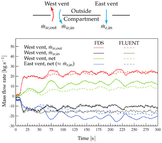
Figure 20.
Same results as in Figure 5b, but obtained with FDS and FLUENT for Case G-4 ().
Despite the discrepancies mentioned above, the overall agreement between FDS and FLUENT is reasonably good. The higher discrepancies between the results of the two codes reported in the literature for some fire simulations, which do not seem to be justified when similar mathematical fire models are solved, might in part be attributed to underresolved numerical solutions in space and/or time obtained with FLUENT, which requires substantially more computational resources than FDS for a given grid resolution. The main disadvantage of FLUENT over FDS, at least for the scenarios simulated and code versions used in this work, is the substantially higher CPU times required (as much as twice or even more) when standard settings are used, a drawback that is not accompanied by appreciable differences in the numerical predictions. However, differences in CPU time consumption should be taken with care since changes in certain settings may produce substantial variations. For example, using the PISO algorithm instead of SIMPLEC for solving the coupling between mass and momentum conservation equations through pressure increases CPU time consumption in FLUENT by a factor of the order of 20%. Choosing different convergence criteria and numerical settings may also result in appreciable variations in CPU time consumption. On the other hand, FLUENT offers much more flexibility in grid generation for arbitrary geometries and postprocessing of results, and makes simulation set up easier than FDS, which requires a more careful specification of boundary conditions and grid partitions. It should also be pointed out that more recent releases of ANSYS FLUENT [43] are likely to improve the performance of the code, specially in terms of the amount of CPU time consumed.
5. Conclusions
The merits of a specialized and a general-purpose code to simulate a fire in the commercial area of an underground intermodal transportation station are investigated using a simplified fire model, whose results have been previously compared with those of an EDC combustion model. The following conclusions can be drawn from the results presented above.
- The simplified fire model yielded results that, far enough away from the fire focus, are in excellent agreement with those obtained using an EDC combustion model, while requiring appreciably lower CPU times. It was also found that, for a given HRR, the results of the simplified fire model are fairly independent of the inlet velocity and temperature of the hot gases introduced at the fire focus.
- The results obtained with FLUENT using the simplified fire model show a reasonable degree of agreement with those obtained with FDS, except regarding the mass flow rates of cold air entering through the natural vents and CO2 mass flow rates through the west vent and forced ventilation grilles, for which some quantitative differences were observed.
- The features that are most sensitive to using the different codes, fire models, computational grids and turbulence model settings are those describing the fire-induced oscillatory flow through the open vents, particularly the mass flow rate of cool air entering the domain. To the best of our knowledge, neither FDS nor FLUENT have previously been used to predict the type of fire-induced oscillatory flows through openings described in this paper, about which there is relatively little information in the literature.
- The dependence of the oscillation frequency on the HRR was in reasonable agreement with the experimental and numerical results reported in the literature.
- For the fire scenarios considered and versions of the codes used in this work, the main advantage of FDS over FLUENT was found to be its substantially lower CPU time consumption. On the other hand, FLUENT allows much more flexibility in grid generation for arbitrary geometries, and the simulation set up can be done more easily in FLUENT than in FDS.
The results presented in this paper provide insight into the relative merits of specialized and general-purpose codes and different fire models, which are frequently used to assess fire safety levels in buildings in order to reduce risk to human life in the case of fire. The future work based on the presented results may be of help in devising fire safety solutions, aimed at limiting the zones of possible escape routes where people’s survival could be compromised in the event of a fire.
Author Contributions
Conceptualization, C.Z., P.G., J.L. and J.H.; Investigation, C.Z., J.L.; Methodology, C.Z., P.G. and J.H.; Visualization, J.L.; Supervision, J.H.; Writing–original draft, C.Z. and J.H.
Funding
This research was funded by Consorcio Regional de Transportes de Madrid, grant number OTRI-FUNED 5510003256.
Acknowledgments
The support of the Consorcio Regional de Transportes de Madrid is gratefully acknowledged.
Conflicts of Interest
The authors declare no conflict of interest.
References
- Custer, R.L.P.; Meacham, B.J. SFPE Engineering Guide to Performance-Based Fire Protection Analysis and Design of Buildings, 2nd ed.; National Fire Protection Association: Quincy, MA, USA, 2007. [Google Scholar]
- Wang, Y.; Jiang, J.; Zhu, D. Full-scale experiment research and theoretical study for fires in tunnels with roof openings. Fire Saf. J. 2009, 44, 339–348. [Google Scholar] [CrossRef]
- National Fire Protection Association. The SFPE Handbook of Fire Protection Engineering, 4th ed.; NFPA: Quincy, MA, USA, 2008. [Google Scholar]
- Beard, A.; Carvel, R. The Handbook of Tunnel Fire Safety; Thomas Telford Publishing: London, UK, 2005. [Google Scholar]
- Morgan, H.P. Design Methodologies for Smoke and Heat Exhaust Ventilation; Technical Report BRE368; Building Research Establishment: Watford, UK, 1999. [Google Scholar]
- Gao, R.; Li, A.; Hao, X.; Lei, W.; Zhao, Y.; Deng, B. Fire-induced smoke control via hybrid ventilation in a huge transit terminal subway station. Energy Build. 2012, 45, 280–289. [Google Scholar] [CrossRef]
- Migoya, E.; Crespo, A.; García, J.; Hernández, J. A quasi-one-dimensional model of fires in road tunnels. Comparison with three-dimensional models and full-scale measurements. Tunn. Undergr. Space Technol. 2009, 24, 37–52. [Google Scholar] [CrossRef]
- Deckers, X.; Haga, S.; Tilley, N.; Merci, B. Smoke control in case of fire in a large car park: CFD simulations of full-scale configurations. Fire Saf. J. 2013, 57, 22–34. [Google Scholar] [CrossRef]
- Tilley, N.; Rauwoens, P.; Merci, B. Verification of the accuracy of CFD simulations in small-scale tunnel and atrium fire configurations. Fire Saf. J. 2011, 46, 186–193. [Google Scholar] [CrossRef]
- Zhang, J.; Weng, J.; Zhou, T.; Ouyang, D.; Chen, Q.; Wei, R.; Wang, J. Investigation on Smoke Flow in Stairwells induced by an Adjacent Compartment Fire in High Rise Buildings. Appl. Sci. 2019, 9, 1431. [Google Scholar] [CrossRef]
- Novozhilov, V. Computational fluid dynamics modeling of compartment fires. Prog. Energy Combust. Sci. 2001, 27, 611–666. [Google Scholar] [CrossRef]
- Olenick, S.M.; Carpenter, D.J. An Updated International Survey of Computer Models for Fire and Smoke. J. Fire Prot. Eng. 2003, 13, 87–110. [Google Scholar] [CrossRef]
- Boroń, S.; Wȩgrzyński, W.; Kubica, P.; Czarnecki, L. Numerical Modelling of the Fire Extinguishing Gas Retention in Small Compartments. Appl. Sci. 2019, 9, 663. [Google Scholar] [CrossRef]
- Wang, Y.; Chatterjee, P.; de Ris, J.L. Large eddy simulation of fire plumes. Proc. Combust. Inst. 2011, 33, 2473–2480. [Google Scholar] [CrossRef]
- Van Maele, K.; Merci, B. Application of RANS and LES field simulations to predict the critical ventilation velocity in longitudinally ventilated horizontal tunnels. Fire Saf. J. 2008, 43, 598–609. [Google Scholar] [CrossRef]
- Vilfayeau, S.; Ren, N.; Wang, Y.; Trouvé, A. Numerical simulation of under-ventilated liquid-fueled compartment fires with flame extinction and thermally-driven fuel evaporation. Proc. Combust. Inst. 2015, 35, 2563–2571. [Google Scholar] [CrossRef]
- Jain, S.; Kumar, S.; Kumar, S.; Sharma, T. Numerical simulation of fire in a tunnel: Comparative study of CFAST and CFX predictions. Tunn. Undergr. Space Technol. 2008, 23, 160–170. [Google Scholar] [CrossRef]
- McGrattan, K.; Hostikka, S.; McDermott, R.; Floyd, J.; Weinschenk, C.; Overholt, K. Fire Dynamics Simulator User’s Guide (FDS Version 6.1.2); National Institute of Standards and Technology (NIST): Gaithersburg, MD, USA, 2014. [Google Scholar]
- McGrattan, K.; Hostikka, S.; McDermott, R.; Floyd, J.; Weinschenk, C.; Overholt, K. Fire Dynamics Simulator Technical Reference Guide. Volume 1: Mathematical Model (FDS Version 6.1.2); National Institute of Standards and Technology (NIST): Gaithersburg, MD, USA, 2014. [Google Scholar]
- FLUENT. User’s Guide 6.3; Fluent Inc.: New York, NY, USA, 2003. [Google Scholar]
- McGrattan, K.; Hostikka, S.; McDermott, R.; Floyd, J.; Weinschenk, C.; Overholt, K. Fire Dynamics Simulator Technical Reference Guide. Volume 2: Verification (FDS Version 6.1.2); National Institute of Standards and Technology (NIST): Gaithersburg, MD, USA, 2014. [Google Scholar]
- McGrattan, K.; Hostikka, S.; McDermott, R.; Floyd, J.; Weinschenk, C.; Overholt, K. Fire Dynamics Simulator Technical Reference Guide. Volume 3: Validation (FDS Version 6.1.2); National Institute of Standards and Technology (NIST): Gaithersburg, MD, USA, 2014. [Google Scholar]
- Hadjisophocleous, G.; Jia, Q. Comparison of FDS Prediction of Smoke Movement in a 10-Storey Building with Experimental Data. Fire Technol. 2009, 45, 163–177. [Google Scholar] [CrossRef]
- Xiao, B. Comparison of Numerical and Experimental Results of Fire Induced Doorway Flows. Fire Technol. 2012, 48, 595–614. [Google Scholar] [CrossRef]
- Blanchard, E.; Boulet, P.; Desanghere, S.; Cesmat, E.; Meyrand, R.; Garo, J.; Vantelon, J. Experimental and numerical study of fire in a midscale test tunnel. Fire Saf. J. 2012, 47, 18–31. [Google Scholar] [CrossRef]
- Zanzi, C.; Mozas, A.; Hernández, J.; García-Hortelano, A.; Aldecoa, J. Smoke and Heat Propagation Modeling in Transportation Interchange Stations Using LES and RANS Methods. In Proceedings of the ASME 2013 International Mechanical Engineering Congress & Exposition, San Diego, CA, USA, 15–21 November 2013. [Google Scholar]
- Deardorff, J.W. Numerical Investigation of Neutral and Unstable Planetary Boundary Layers. J. Atmos. Sci. 1972, 29, 91–115. [Google Scholar] [CrossRef]
- McGrattan, K.B.; Baum, H.R.; Rehm, R.G. Large eddy simulations of smoke movement. Fire Saf. J. 1998, 30, 161–178. [Google Scholar] [CrossRef]
- Magnussen, B.; Hjertager, B. On mathematical modeling of turbulent combustion with special emphasis on soot formation and combustion. Symp. (Int.) Combust. 1977, 16, 719–729. [Google Scholar] [CrossRef]
- Raithby, G.D.; Chui, E.H. A Finite-Volume Method for Predicting Radiant Heat Transfer in Enclosures with Participating Media. J. Heat Transf. 1990, 112, 415–423. [Google Scholar] [CrossRef]
- Hopkin, C.; Spearpoint, M.; Hopkin, D. A Review of Design Values Adopted for Heat Release Rate Per Unit Area. Fire Technol. 2019. [Google Scholar] [CrossRef]
- Haynes, W.E. CRC Handbook of Chemistry and Physics, 94th ed.; CRC Press LLC: Boca Raton, FL, USA, 2014. [Google Scholar]
- Cox, G.; Kumar, S. Modelling Enclosure Fires Using CFD. In SFPE Handbook of Fire Protection Engineering, 3rd ed.; NFPA: Quincy, MA, USA, 2002; Chapter 3–8; pp. 194–218. [Google Scholar]
- Smoke and Heat Control Systems—Part 3: Specification for Powered Smoke and Heat Control Ventilators (Fans); Norma Europea UNE-EN 12101-3:2016; Asociación Española de Normalización: Madrid, Spain, 2016.
- Baum, H.R.; McCaffrey, B.J.F. Fire Induced Flow Field—Theory and Experiment. In Fire Safety Science, Proceedings 2nd International Symposium; Hemisphere: New York, NY, USA, 1989; pp. 129–148. [Google Scholar]
- Cooper, L.Y. Combined Buoyancy and Pressure-Driven Flow Through a Shallow, Horizontal, Circular Vent. J. Heat Transf. 1995, 117, 659–667. [Google Scholar] [CrossRef][Green Version]
- Chow, W.K.; Gao, Y. Oscillating behaviour of fire-induced air flow through a ceiling vent. Appl. Therm. Eng. 2009, 29, 3289–3298. [Google Scholar] [CrossRef]
- Chow, W.K.; Gao, Y. Buoyancy and inertial force on oscillations of thermal-induced convective flow across a vent. Build. Environ. 2011, 46, 315–323. [Google Scholar] [CrossRef]
- Tan, Q.; Jaluria, Y. Mass flow through a horizontal vent in an enclosure due to pressure and density differences. Int. J. Heat Mass Transf. 2001, 44, 1543–1553. [Google Scholar] [CrossRef]
- Satoh, K.; Matsubara, Y.; Kumano, Y. Flow and Temperature Oscillations of Fire in a Cubic Enclosure with a Ceiling and Floor Vent. Part I. In Technical Report 55, Report of Fire Research Institute of Japan; Fire Research Institute: Tokyo, Japan, 1983. [Google Scholar]
- Satoh, K.; Lloyd, J.R.; Yang, K.T. Flow and Temperature Oscillations of Fire in a Cubic Enclosure with a Ceiling and Floor Vent. Part III. In Technical Report 57, Report of Fire Research Institute of Japan; Fire Research Institute: Tokyo, Japan, 1984. [Google Scholar]
- Kerrison, L.; Galea, E.R.; Patel, M.K. A two-dimensional numerical investigation of the oscillatory flow behaviour in rectangular fire compartments with a single horizontal ceiling vent. Fire Saf. J. 1998, 30, 357–382. [Google Scholar] [CrossRef]
- ANSYS Fluent. User’s Guide, Release 2019 R2; ANSYS, Inc.: Canonsburg, PA, USA, 2019. [Google Scholar]


© 2019 by the authors. Licensee MDPI, Basel, Switzerland. This article is an open access article distributed under the terms and conditions of the Creative Commons Attribution (CC BY) license (http://creativecommons.org/licenses/by/4.0/).