An Accurate Prediction of Daylight Pipe Harvesting of Interior Space

Featured Application

The results of this research are useful in correct assessment of daylighting quality in the interiors respecting the typical instability of sky states. The computations we have performed allow for designing the optimum energy-saving solutions for light-pipe systems.

Abstract

The performance of a light guide under arbitrary meteorological conditions is difficult to predict numerically because none of the present methods can account for the random configuration of clouds. Although, partly cloudy skies typically occur very frequently in many regions over the globe, the effects of cloud sizes, distributions, or altitudes on the luminous effectiveness of a light guide remain virtually unknown. The physical installation of light guides does not allow for a controlled experiment in which a single parameter can be varied within a defined range, while holding all other parameters constant. Numerical modeling is the only practical way to provide deep insights on the role of a specific property, such as cloud coverage, and its importance relative to all others (e.g., atmospheric turbidity). We have developed a unique solution through linking the UniSky simulator and HOLIGILM (hollow light guide interior illumination method) tool, while providing for the first time a powerful method that can provide accurate predictions and understanding of the fundamental differences of light guide behaviors under homogeneous and inhomogeneous sky states. The use of homogeneous skies in low-accuracy empirical models often results in overestimated/underestimated effectiveness of some light-guide systems. The model we have developed can predict complex optical signatures that are normally impossible to reproduce using up-to date empirical models (e.g., the illuminance patterns due to isolated clouds or clouds traversing across the sky). The optical efficiency, average cosine and working-place illuminance are analyzed and compared in order to demonstrate the model capabilities.

1. Introduction

The need for adequate illumination in building interiors, building cores, deep offices or halls has escalated in the last few decades due to the rapid spread of densely built-up areas worldwide. The use of electric lights can solve the problem [1,2], but typically results in wasting energy [3,4], and in the loss of natural light that otherwise makes the interior environment more desirable for human activities and health.

Light-guide systems can deliver natural light into rooms (Figure 1) and mimic the dynamics of external illumination conditions [5,6]. Light pipe is a desirable technology because it does not impose an additional burden on energy sources and has no negative impact on the natural environment [7,8]. The performance of such a passive system depends mainly on the transmission properties of the light-guide body, but also on the instantaneous meteorological conditions [9,10,11,12]. The optical parameters of straight pipes have been intensively studied by many authors [13,14,15,16,17], while some have demonstrated that clear skies more than overcast ones produce complex illuminance patterns in the interior spaces. Illuminance levels, the angular distribution of light and also its dynamics altogether affect both the visual comfort and working conditions in a room. No doubt that interior illuminance is undergoing large changes during optically unstable days characterized by broken cloud arrays with bright sky windows between isolated clouds. Such heterogeneous cloud fields present the largest uncertainty in modeling the light-pipe efficiency and thus deserve a special attention. Nevertheless, no quantification of the light-pipe efficiency for in-lab simulated heterogeneous cloud distributions exists, and no fully controlled experiment is possible in the exterior. Such an experiment does not satisfy one (or even both) of the basic preconditions: (a) All atmospheric parameters must be a-priori known, and, (b) only a single parameter (e.g., cloud arrangement, or aerosol content) can be varied within a defined range, while all other parameters should be kept constant during the experiment.

The models currently in use predict the optical effects from the CIE skies (sky types standardized by International Commission on Illumination), which are homogeneous in terms of luminance patterns. In these models any irregularities due to the presence of isolated clouds with distinct edges are ignored, so the luminance patterns are smooth and may largely differ from what we can observe under real conditions. However, the broken cloud arrays are recognized to have a great impact on the luminance distribution and thus a potentially great unknown impact on the light field at the lower interface of the light-pipe. Due to this reason the range of illuminance signatures we can expect from heterogeneous cloud fields remains unexplored. This problem requires a proper treatment to either improve the accuracy of numerical predictions of interior illuminance or to understand the limits of the models of homogeneous skies.

For the first time, we treat the light field below a tubular pipe theoretically and numerically for random cloud arrangements taking into account inhomogeneous sky radiance patterns changing abruptly at the edges of each single cloud. We analyze a straight vertical pipe, which is a first step for the characterization of more complex systems. We address the principal question: What are the main differences between the light-guide optical signatures under a homogeneous sky and the fractional cloud cover with individual clouds distributed randomly over the sky. Among all homogeneous skies, the most known are Kittler’s system of sky standards [18] and Perez’s model of sky luminance distributions [19]. It is still unclear how the light-pipe optics changes depending on the cloud coverage and sun position relative to the cloud field. Such analysis is difficult to perform experimentally, because optical signatures observed in a room interior are the result of complex interactions of various parameters that all can change concurrently. It is rather impossible to isolate the contribution from only one parameter to the illuminance pattern, while holding all other factors constant. The comprehensive understanding of what is the role of clouds in shaping the interior illuminance is only possible in a controlled numerical experiment that is performed in this paper.

No doubt that the light pipe installations in buildings routinely include a transparent dome at the upper interface and a diffusing component at the lower interface. Nevertheless, we intentionally avoided these two components in order to understand better the optical signatures due to clouds. It has to be emphasized that a diffusing cover suppresses the amplitude of the optical signal and distorts the light field below the light-pipe. This can make the proper analysis of cloud effects largely impossible. The analysis made for a specific diffuser would not be as general as it could be, while the findings would be limited to only a specific configuration of the light-guide system. In contrast, the understanding of how the conversion from a specific sky luminance pattern to the illuminance pattern in the interior space works is necessary for modeling the light field in situations with and without the diffusing cover. The modeling in this paper is specifically oriented towards the effects from broken clouds and eliminates all other (potentially parasitic) effects.

2. Theoretical Framework

The photons on their path undergo a scattering, reflection and absorption phenomena before they are transported from the sky to a building interior. The light scattering within the Earth’s atmosphere and also the diffuse reflection from the clouds are by far the most important factors influencing the ground-reaching radiation; however, the absorption by aerosols can also play an important role especially in densely polluted (industrial) regions. The light guide can be fully characterized by its optical properties and boundary conditions, such as the light field entering the pipe at its upper interface. The latter can be predicted from the UniSky Simulator which is designed to model radiance patterns under arbitrary sky conditions [20].

2.1. Radiance Field below an Inhomogeneous Cloud Field

Modeling the light output from a heterogeneous system of broken cloud arrays is a nontrivial problem because the clouds can differ in size, shape and also spatial distribution. We treat the problem within the framework of the successive orders of scattering (SOS) which is the method to calculate the total sky radiance as an infinite series of higher-order scattering components. However, it has been shown that the contribution to the radiance from the clouds and cloudless atmosphere can be separated [21], thus taking advantage of low eigenvalues for an optically thin atmosphere [22]. Due to fast convergence, the model can be limited to the first two scattering modes, so the truncated series for total sky radiance reads

$$L_{e,\lambda }^{+}={\displaystyle \sum }_{i=1}^{\infty }{L}_{e,i,\lambda }^{+}\cong L_{e,1,\lambda }^{S+}+L_{e,2,\lambda }^{S+}+L_{e,1,\lambda }^{R+}+L_{e,2,\lambda }^{R+}+L_{e,1,\lambda }^{T+},$$

(1)

where the symbol (+) indicates the downward radiance, while the superscripts S, R, and T are for the scattered, reflected and transmitted components of the ground-reaching radiance. The R and T components characterize the radiance of a cloud, $L_{e,1,\lambda }^{S+}$ is for the first-scattering radiance of a cloud-free atmospheric window, and $L_{e,2,\lambda }^{S+}$ is the second-scattering radiance obtained as a non-trivial integral product of all first-scattering radiances (i.e., all combinations of upward and downward S, R, and T radiance components). Each of the $L$—components is formulated as a function of observational zenith and azimuth angles accepting the momentary sun position and altitude of a hypothetical observer [21]. In this way Equation (1) can provide sky radiance patterns under any cloudiness and turbidity conditions in lowland or mountain sites.

One of the key elements in the theory is to characterize the stochastic cloud fields through a cloud-masking algorithm that is aimed to predict the presence of clouds along the line of sight. The UniSky Simulator provides a general solution for arbitrary cloud distributions, but a significant reduction of the CPU and MEM consumptions can be achieved by introducing azimuthal averaging over the cloud arrays. For instance, Zuev and Titov [23] have approximated the probability function for cloud visibility as follows:

$${\delta }_{0,z}=1-\left(1-C_F\right)e^{C_F\beta \left(\sec z-1\right)},$$

(2)

where $C_F$ is the so-called nadir-view cloud fraction [24] and $\beta$ is the ratio of the horizontal to vertical cloud dimensions.

The cloud field significantly influences the diffuse component of the ground-reaching radiation, but tools that simulate the ground irradiance accurately are rare. We have developed a CPU-non-intensive method to compute the angular distribution of the scattered radiation under broken cloud arrays taking advantage of the concept of the successive orders of scattering that allows for separation of higher-scattering radiances from the broken clouds and cloud-free atmosphere. Reference [21] has shown that the numerical computations can be accomplished rapidly using an inexpensive Intel Pentium processor. Such a rapid algorithm is ideally suited for solving complex problems of daylight propagation into interior spaces through a light-pipe system.

Most typically, the horizontal irradiance/illuminance is used as an input to many tools modeling the optical efficiency of straight light pipes. The optical efficiency is defined as the ratio of the luminous flux at the light-tube exit relative to that at the light-tube entrance. Based on the above theoretical model the diffuse horizontal component of the solar radiation is obtained as the cosine-projected spectral radiance integrated over the upper hemisphere, i.e.,

$$D_H=\underset{z=0}{\overset{\pi /2}{{\displaystyle \int }}}\sin z\cos z\left\{\underset{A=0}{\overset{2\pi }{{\displaystyle \int }}}{L}_{e,\lambda }^{+}\left(z,A\right)dA\right\}dz.$$

(3)

where A and Z are the azimuth and zenith angle of a sky element, respectively. In daylight science and daylighting technology we deal with the diffuse horizontal illuminance $D_{V,H}$ rather than the spectral irradiance $D_H$. $D_{V,H}$ can be obtained by integrating the above formula over the visible spectrum taking into account the photopic spectral luminous efficiency $V\left(\lambda \right)$ of an individual observer, i.e.:

$$D_{V,H}=683\underset{380 nm}{\overset{780 nm}{{\displaystyle \int }}}{D}_{H}V\left(\lambda \right)d\lambda .$$

(4)

Direct sunlight is determined as a luminance of a finite-dimensional solar disk, whose position is characterized by the azimuth angle $A_S$ and the zenith angle $z_S$ as well. The direct normal illuminance in a turbid atmosphere with optical thickness of ${\tau }_0$ is

$$E_{V,S}=E_V exp\left\{-\frac{{\tau }_0}{\cos z_S}\right\},$$

(5)

where $E_V$ is the normal extraterrestrial illuminance due to sunlight. The solar luminance $L_{V,S}$ can be determined from the ground illuminance $E_{V,S}$ normalized to the solid angle of the sundisk, i.e.,

$$L_{V,S}=E_{V,S} \frac{1}{2\pi \left(1-\cos {\Re }_S\right)},$$

(6)

where ${\Re }_S$ is the angular radius of the sun (approximately 16 angular min).

2.2. Light Transmission through a Straight Light Guide

Tubular light guides harvest the diffuse light and sunlight and transport the photons into building interiors through the tube’s inner high-reflecting coating. Following the analytical model [25], the luminous flux crossing the circular interface at the light-tube base can be written as

$${\mathsf{\Phi }}_D=\frac{1}{2}\underset{r_0=0}{\overset{R}{{\displaystyle \int }}}{r}_{0}d{r}_0\underset{{\varphi }_0=0}{\overset{2\pi }{{\displaystyle \int }}}d{\varphi }_0\underset{\theta =0}{\overset{\pi /2}{{\displaystyle \int }}}\sin \left(2\theta \right)d\theta \underset{\phi =0}{\overset{2\pi }{{\displaystyle \int }}}j\left(\theta ,\phi ,{\varphi }_0,r_0\right)d\phi ,$$

(7)

where $R$ is the radius of the circular diffuser embedded at the light-tube base, $r_0$ is the radial distance measured from the center of the diffuser to an elementary area on its surface, ${\varphi }_0$ is the polar angle of the elementary area, and, $\theta$ and $\phi$ are the apparent zenith and azimuth angles of a light beam that enters the elementary area from upwards, respectively. The luminance at the light-tube base $j\left(\theta ,\phi ,{\varphi }_0,r_0\right)$ is proportional to the sky luminance reduced primarily due to the multiple reflections in a tube and attenuation in the hemispherical top dome. The illuminance of the elementary surface of the diffuser in local coordinates ${\varphi }_0,$ $r_0$ is

$$E_i\left({\varphi }_0,r_0\right)=\underset{\theta =0}{\overset{\pi /2}{{\displaystyle \int }}}\underset{\phi =0}{\overset{2\pi }{{\displaystyle \int }}}j\left(\theta ,\phi ,{\varphi }_0,r_0\right)\cos \theta \sin \theta d\theta d\phi .$$

(8)

For a vertical straight pipe, the polar angle of a light beam $\theta$ is conserved in the process of multiple reflections, i.e., the exit angle equals to the entrance angle. The illuminance below the diffuser-free light-guide can be determined easily for any point $X^{\prime },Y^{\prime },Z\prime$ in the work plane:

$$\begin{gathered} E_W\left(X^{\prime }, Y^{\prime },Z^{\prime }\right)=\frac{t_D}{2\pi }\underset{r_0=0}{\overset{R}{{\displaystyle \int }}}{r}_{0}d{r}_0\underset{{\varphi }_0=0}{\overset{2\pi }{{\displaystyle \int }}}\frac{{\cos }^2\mathsf{\Theta }}{D^2\left(\mathsf{\Theta },\mathsf{\Phi },r_0,{\varphi }_0\right)}d{\varphi }_0 \\ \underset{\theta =0}{\overset{\pi /2}{{\displaystyle \int }}}\sin \left(2\theta \right)d\theta \underset{\phi =0}{\overset{2\pi }{{\displaystyle \int }}}j\left(\theta ,\phi ,{\varphi }_0,r_0\right)d\phi , \end{gathered}$$

(9)

where $D$ is the distance between a point on the light tube base and arbitrary point at the work plane. The angles $\mathsf{\Theta },\mathsf{\Phi }$ are to characterize the direction of the beam propagation below the light-pipe.

In previous equations, the luminance $j\left(\theta ,\phi ,{\varphi }_0,r_0\right)$ is obtained as a function of the zenith and azimuth angles and also depends on the point in which the beam intersects the upper interface of a light-pipe. When the sunlight is absent, we can write

$$j\left(\theta ,\phi ,{\varphi }_0,r_0\right)=L_a{\rho }^N{t}_C,$$

(10)

where the luminance of sky element $L_a$ can be computed from the UniSky model as a sum of the first-order and the second-order luminance components (see Equation (1)). The reflectance of a light-tube interior surface is characterized by $\rho$ that is considered to be constant. The same applies to the transmission coefficient of a hemispherical cupola ($t_C$). However, the number of reflections $N$ depends on the geometry of the light guide and incidence angle (for more details see [25]. The contribution from the direct sunlight to the luminance is

$$j_S\left(\theta ,\phi ,{\varphi }_0,r_0\right)=\frac{L_{V,S}}{\cos z_S}{\rho }^{N_{sun}\left(\phi \right)}{t}_C,$$

(11)

while $L_{V,S}$ is determined from Equation (6), and $N_{sun}$ can be computed analogously to $N$ assuming the zenith and azimuth angles coincide with the position of sun.

3. The Variety of Effects the Broken Cloud Arrays Could Have on a Light Field

Based on the aforementioned theoretical approaches, the UniSky tool [20] has been linked to the HOLIGILM tool [25]. The UniSky solution provides the zenith-normalized spectral sky radiance or luminance distributions, accepting the optical properties of a local atmosphere. Some of these properties vary only slightly over time, but others depend strongly on time and place. The HOLIGILM is used for modeling the light transmission through the tubular light guide with a hemispherical top dome and allows for different types of diffusers. Using this tool we can test various tube adjustments by altering the tube radius, length and inner surface reflectance. In addition, the optical properties of the cover dome and diffuser can be varied, taking into account different positions of the sun and different luminance patterns under arbitrary atmospheric conditions. We have analyzed the most typical atmospheric conditions aiming to demonstrate the role broken cloud arrays play in forming the illuminance patterns below a straight light pipe. It is ideal to keep the bottom interface of a light tube open in order to illustrate the effects the clouds could have on the illumination scene in the interior. Note that the Lambertian diffusers distribute the light homogeneously in all directions, thus efficiently suppressing daylight dynamics that is typical for natural conditions outdoors.

Among many others, the UniSky simulator also uses a set of parameters to model light scattering in a turbid atmosphere. The most important ones are shortly introduced below. The total optical thickness of a cloud-free atmosphere, ${\tau }_0,$ is due to the trivial superposition of the Mie and Rayleigh optical depths. The asymmetry factor $g\prime$ and the single scattering albedo ${\omega }_0$ are key parameters for modeling the light scattering in a cloud free atmosphere. The parameter $g\prime$ is used to characterize the scattering function, while ${\omega }_0$ is the ratio of the scattering efficiency to the extinction efficiency. Unless it is stated otherwise, the most typical values for the Central European region (${\tau }_0$ = 0.3; $g\prime$ = 0.65; ${\omega }_0$ = 0.85) are used in our simulations. Other parameters particularly important for further computations are as follows: The altitude of a cloud base $H_C,$ cloud radius $R_C,$ cloud albedo ${\rho }_C,$ and cloud fraction $C_F$. The cloud fraction varies from zero to one, where zero refers to a cloudless sky and one is for a completely overcast sky. Input parameters to the HOLIGILM tool are as follows: Tube length $l,$ tube radius $r,$ inner reflectance of the tube $\rho ,$ optical transparency of the top dome $t_C,$ diffuser type and room dimension $\left(x,y\right)$. To be consistent with our previous studies we use the following: $H$ = 1.5 m, $r$ = 0.26 m, $\rho$ = 0.934, $t_C$ = 0.92, $x$ = 6 m and $y$ = 4 m. The position of the light guide center with respect to the center of the room coordinate system is $x\prime$ = 1.5 m and $y\prime$ = 2 m. The vertical separation of the room ceiling and work plane is 3 m.

3.1. Sky Luminance Distribution

The sky luminance distributions were calculated for solar coordinates ($A_S$ = 180°, $z_S$ = 60°) and three nadir-view cloud fractions: (a) 0.15, (b) 0.30 and (c) 0.45. Assuming the cloud-base altitude is $H_C$ = 1 km and the cloud radius is $R_C$ = 0.5 km, the respective hemispherical sky cover fractions ($C_{F,hemisf}$) are as follows: (a) 0.22, (b) 0.45, and (c) 0.67. The clouds situated opposite to the position of the sun can contribute essentially to the ground-reaching radiation if the sun is low and cloud albedo ${\rho }_C$ > 0.5 (see Figure 2). Therefore, the beams of light entering the upper interface of a straight pipe from the anti-solar quadrant can have an important contribution to the light field below the pipe. It is also shown in Figure 2 that the luminance typically drops as the cloud fraction increases.

3.2. Work Plane Illuminance

The illuminance patterns mimic the dynamics of cloud fields, especially if the cloud fraction exceeds the value of 0.3. Therefore, a special diffuser composed of transparent and Lambertian parts [26] may appear useful in regions where the sun is preferably low. The sky luminance distributions and work-plane illuminance levels computed for various cloud fractions and a solar altitude at 45° are shown in Figure 3. In this numerical experiment we assume the solar disk is not masked by clouds, resulting in a bright ring projected onto a work plane during sunny days. However, the illuminance below a light tube can increase monotonically as the cloud fraction approaches elevated values (see Figure 3a–d). The central brightening is manifested in Figure 3d, where the cloud fraction is as large as 0.45.

The optical effects of the clouds are amplified as the sun elevation decreases (see Figure 4). In such cases the low beams do not provide sufficient illumination because of multiple reflections in a vertical tube. However, the intensity distribution below the tube could change with the cloud fraction. High cloud fractions typically favor high illuminance levels near the optical axis of the light tube to the detriment of an originally bright ring; compare Figure 4a with Figure 4d. The bright ring disappears in Figure 4d due to the absent sunlight.

A central brightening and azimuthal symmetry of illuminance patterns are both observed for situations with random cloud distributions. Such effects are due to multiple reflections of light when travelling through a light-tube. The sky luminance distributions are displayed in Figure 4.

3.3. The Clouds Traversing the Sky from or to a Preferred Quadrant

The sky radiance patterns due to the clouds drifting from a preferred direction can differ from what we can observe for random cloud distributions. Such a cloud-field movement is frequently observed in Central Europe during sunset or sunrise. The UniSky tool can model this situation using two parameters: (1) Preferred direction—which is the azimuth position of a cloud array, and, (2) preferred direction ratio—which is the probability that a cloud array occurs at the preferred hemisphere. The latter parameter ranges from 0% to 100%. We also introduce a direction offset that defines the transition from the preferred to non-preferred part of the sky. The clouds group near the horizon if the offset is a positive value.

The sky luminance distributions and interior illuminance below a light pipe are analyzed in Figure 5 for the cloud fields near solar and anti-solar positions, while the preferred direction ratio is 100% and the cloud offset is 2 km. All other inputs parameters are kept as before. The position of the sun is ($z_S$ = 20°, $A_S$ =180°), and the preferred directions of the cloud field are 0° for Figure 5a and 180° for Figure 5b, respectively. Note that the magnitude of the illuminance on the work plane under these conditions is quite low—only a fraction of what would typically be desired for the interior office work. Figure 3, Figure 4 and Figure 5 are, however, to demonstrate the range of optical signatures we can expect under different conditions, i.e., to document the changes when transitioning from an intense ring-shaped illuminance pattern to a more homogeneous circular pattern with characteristic low illumination levels.

Figure 5 demonstrates the changes of illumination patterns associated with the cloud arrangement. Due to the complex optical transform from the sky radiance distribution to the room illuminance map, the peak intensities can be also observed at the side opposite to the azimuthal position of the cloud array; however, the amplitudes of these optical effects strongly depend on the position of the clouds relative to the sun (compare Figure 5a,b).

4. Comparison of Light-Tube Optical Properties under Arbitrary and Homogenous Skies

Simple models of homogeneous skies are still preferred, most likely because of easy implementation and rapid computations. However, the computers are now fast and inexpensive, so there is no significant reason for insisting upon tools with low-accuracy levels. Accurate models of heterogeneous cloud fields are necessary because such conditions occur over 50% of the globe at any time. Inhomogeneous sky situations dominate in many regions. A demand to use the models of homogeneous skies in such situations can result in inaccurate predictions of interior illuminance due to differences between the real and approximated sky luminance fields. It is our intention to inspect the range of errors induced in this approximation. To do this, we compare the exact computations based on the UMRP (Unified Model of Radiative Patterns) of heterogeneous cloud fields [27] against a well-known all-weather model of homogeneous skies [19]. Note that Perez’s model is commonly used in many applications and is designed to predict the sky luminance from the global and direct irradiance data and dew point temperature. The latter is calculated from humidity and real temperature, while the insolation conditions are determined from the solar zenith angle Z_S, Perez’s sky clearness $\epsilon ,$ and Perez’s sky brightness $\Delta$. The UMRP computes the spectral sky radiance for arbitrary cloud coverage using aerosol and cloud parameters as inputs. The conversion from radiance to luminance is possible through the average spectral sensitivity of the human visual perception of brightness, i.e., the V($\lambda$) function. The luminance distributions determined from Perez’s all-weather model and UMRP are linked with the HOLIGILM tool in order to model the light field below a light guide length of H = 1.5 m, radius r = 0.26 m and internal specular reflectance $\rho$ = 0.934. We avoid a diffusing cover to better understand the work plane illuminance data obtained from numerical runs assuming various sky conditions. The transparency of a hemispherical top dome (0.92) is fixed for all the model computations.

4.1. Clear and Overcast Skies

It is a natural goal of all the luminance models to mimic a momentary sky state as accurately as possible. Of all cases, the clear and overcast skies represent the best conditions to test different models, because we avoid random errors that can originate from the missing information on the cloud arrangement. The common requirement is to test the models on real data and in situations that regularly occur in nature. We have used the optical data taken in Bratislava, Slovakia. Of all the data taken during a reference year we have selected two days that are well representative for clear and overcast conditions.

The horizontal global ($G_h$) and diffuse ($D_h$) irradiance data needed to run Perez’s model are shown in

Table 1. Data collected at the Slovak Hydro-meteorological Institute (Bratislava, Slovakia) on 16 February 2015 under clear sky conditions: $A_S$—azimuth of the sun, $z_S$—solar zenith angle, $G_h$—global horizontal irradiance, $D_h$—diffuse horizontal irradiance, $t$ —air temperature, $RH$—relative humidity, $C_F$—cloud fraction. Time is given in the coordinated universal time (UTC).

Time (UTC)	${\mathit{A}}_{\mathit{S}}$ (deg)	${\mathit{z}}_{\mathit{S}}$ (deg)	${\mathit{G}}_{\mathit{h}}$ (W.m−2)	${\mathit{D}}_{\mathit{h}}$ (W.m−2)	$\mathit{t}$ (°C)	RH (%)	${\mathit{C}}_{\mathit{F}}$ (-)
7:00	120.04	81.56	113.77	38.03	2.5	61	0
8:00	132.55	73.50	265.25	52.69	4	56	0
9:00	146.49	67.00	388.61	63.88	6.9	49	0
10:00	161.93	62.64	476.91	68.31	6.9	48	0
11:00	178.43	60.92	505.98	66.43	7.7	47	0
12:00	195.03	62.10	484.00	68.31	8.4	45	0
13:00	210.72	66.00	404.05	61.76	9.4	44	0
14:00	224.95	72.14	282.90	58.68	8.8	43	0
15:00	237.71	79.95	134.30	46.88	7.9	54	0

and

Table 2. The same as in Table 1, but for 24 February 2015 (overcast sky).

Time (UTC)	${\mathit{A}}_{\mathit{S}}$ (deg)	${\mathit{z}}_{\mathit{S}}$ (deg)	${\mathit{G}}_{\mathit{h}}$ (W.m−2)	${\mathit{D}}_{\mathit{h}}$ (W.m−2)	$\mathit{t}$ (°C)	RH (%)	${\mathit{C}}_{\mathit{F}}$ (-)
7:00	118.46	79.15	26.31	26.31	3.9	97	1
8:00	131.19	70.94	48.97	48.97	4.2	97	1
9:00	145.47	64.28	82.91	82.91	4.7	97	1
10:00	161.43	59.80	82.93	82.93	5.4	96	1
11:00	178.58	58.06	147.44	147.44	6.1	96	1
12:00	195.83	59.32	137.28	137.28	6.0	91	1
13:00	212.03	63.39	83.94	83.94	5.6	89	1
14:00	226.60	69.73	71.96	71.96	5.2	91	1
15:00	239.55	77.73	31.44	31.44	5.1	90	1

. Note that the dew point temperature is calculated from the relative humidity RH and real temperature $t$ using Equation (11) in [28]. The sky clearness index $\epsilon$ and sky brightness $\Delta$ computed for both the clear and overcast skies are presented in

Table 3. The input data to Perez’s all-weather model ($\Delta ,$ $\epsilon$) and UMRP model ($h_C,$ $r_C,$ ${\tau }_a,$ $g\prime ,$ ${\omega }_0$) for 16 February 2015 under clear sky conditions: $\Delta$—sky brightness, $\epsilon$—sky clearness, $h_C$—cloud base altitude, $r_C$—cloud radius, ${\tau }_a$—aerosol optical depth, $g^{\prime }$—aerosol asymmetry parameter, ${\omega }_0$—single scattering albedo of aerosol particles, Dev.—deviation between the experimentally determined irradiance data and those simulated using the UMRP model. Time is given in the coordinated universal time (UTC).

Time (UTC)	${\mathit{h}}_{\mathit{C}}$ (km)	${\mathit{r}}_{\mathit{C}}$ (km)	${\mathit{\tau }}_{\mathit{a}}$ (-)	${\mathit{g}}^{\prime }$ (-)	$\mathit{\omega }$ (-)	$\Delta$ (-)	$\mathit{\epsilon }$ (-)	Dev. (%)
7:00	-	-	0.11	0.82	0.82	0.178	4.377	1.38
8:00	-	-	0.11	0.82	0.68	0.131	5.440	0.25
9:00	-	-	0.01	0.89	0.98	0.116	5.881	1.22
10:00	-	-	0.21	0.96	0.42	0.106	6.514	0.11
11:00	-	-	0.41	0.68	0.42	0.097	7.037	1.39
12:00	-	-	0.11	0.41	0.82	0.104	6.592	1.15
13:00	-	-	0.11	0.68	0.68	0.108	6.259	0.86
14:00	-	-	0.11	0.68	0.82	0.135	5.047	1.03
15:00	-	-	0.11	0.82	0.96	0.187	3.781	1.77

and

Table 4. The same as in Table 3, but for 24 February 2015 (overcast sky).

Time (UTC)	${\mathit{h}}_{\mathit{C}}$ (km)	${\mathit{r}}_{\mathit{C}}$ (km)	${\mathit{\tau }}_{\mathit{a}}$ (-)	$\mathit{g}\prime$ (-)	$\mathit{\omega }$ (-)	$\Delta$ (-)	$\mathit{\epsilon }$ (-)	Dev. (%)
7:00	1.1	2.4	0.01	0.4	0.4	0.099	1.000	1.80
8:00	0.6	1.0	0.01	0.4	0.4	0.107	1.000	0.34
9:00	0.7	0.9	0.01	0.4	0.4	0.136	1.000	1.05
10:00	0.7	0.9	0.01	0.4	0.4	0.118	1.000	1.90
11:00	1.4	0.6	0.01	0.4	0.4	0.199	1.000	1.49
12:00	1.3	0.7	0.01	0.4	0.4	0.192	1.000	1.93
13:00	0.7	0.9	0.01	0.4	0.4	0.134	1.000	1.70
14:00	0.8	0.6	0.01	0.4	0.4	0.148	1.000	0.44
15:00	0.5	1.0	0.01	0.4	0.4	0.106	1.000	0.80

, showing that $\epsilon$ is one when the cloud fraction approaches unity. However, $\epsilon$ can fluctuate as a result of the evolving atmospheric turbidity (see e.g., Table 3). The aerosol optical depth has increased shortly before noon, but then remained constant and equal to that of the morning value (0.11). Peak values at noon normally occur due to intensified turbulent mixing in the boundary layer or due to the change of wind direction. The wind direction is often associated with changes of aerosol content and origin, especially if the measuring site is surrounded by different pollution sources. This was just the case in our field experiment that has been performed in the city of Bratislava with many industrial and anthropogenic emission sources. Other evidence for a transform of aerosol system is that the single-scattering albedo of aerosol particles (${\omega }_0$) has changed abruptly when ${\tau }_a$ achieved peak values. The transition from ${\omega }_0$ > 0.7 in the morning to ${\omega }_0$ ≈ 0.4 at noon can be interpreted as a contamination of the local aerosol population by highly absorbing particles, most probably due to emissions from close industrial sources. At the same time, the asymmetry parameter of aerosol particles $g\prime$ drops down from almost 0.9 to 0.7 and then to 0.4, meaning that the concentration of the small particles has increased. This is consistent with the experimental studies indicating that most of the absorbing particles (e.g., some fractions of carbonaceous species) are small in size [29,30]. The values of ${\tau }_a$ which are all found to be nearly zero under overcast sky conditions (Table 4) indicate that the aerosol content was at the detection limit. This is not surprising, because low-level clouds with a base below 2 km are often rainy and contribute to the efficient removal of tiny particles in the under-cloud atmosphere through frequent rainfall.

The accuracy of the UMRP model is demonstrated in Table 3 and Table 4, where the parameter Dev is obtained by matching the modelled to the measured irradiance data. The deviation obtained is as low as 1%, implying that UMRP is capable of simulating both clear and overcast sky conditions with exceptional accuracy.

Figure 6 and Figure 7 demonstrate that for the homogeneous skies, there is not much difference between the optical properties of the light guides simulated using the UMRP and Perez’s model. In general, Perez’s model works well and the small differences found are due to its physical limits or variability of input parameters (e.g., altitude of the cloud base in the case of the overcast sky; see Figure 7). It is symptomatic for the clear sky that the optical efficiency of a vertical tubular light guide peaks when the sun is high. This feature has been reproduced by the UMRP and Perez’s model in a consistent way. On the other hand, the illumination scene below a straight light pipe is normally conserved under overcast sky conditions. However, Perez’s model is unable to mimic changes in cloud altitudes. We have computed the average cosine, a parameter that characterizes the directionality of light at the exit from the bottom interface of a light guide. For more details on the fundamentals of the average cosine, <cos>, see [31]. <cos> approaches unity if all the photons propagate axially and thus illuminate the small circular area just below the pipe. <cos> monotonically decreases when the angle from the axis increases; and <cos>=0 is for a pipe that emits all the photons horizontally while illuminating the walls rather than the work plane. It is natural that the luminous energy entering the light tube at its top is never exclusively transmitted to a single direction. The beams of light spread over a wide range of angles, so the <cos> characterizes the direction of the peak luminous flux. The cosine of the angle is a dimensionless quantity and always ranges from zero to one. <cos> for the clear sky is slightly smaller than that for the overcast sky (compare Figure 6b and Figure 7b), meaning that the overcast sky preferably illuminates the work plane near the axis of the pipe. The <cos> we have found under cloudless conditions can be even smaller than 0.5, especially when the sun is low and the local atmosphere is clean. In such cases the direct sunbeams dominate all other sources of illumination (diffuse or reflected light).

4.2. Partly Cloudy Days

It is not uncommon that the model of the homogeneous skies works well under stable cloudless and overcast conditions. However, the sky state is usually heterogeneous in many regions with arbitrary cloud configurations. This makes the availability of direct sunbeams very irregular. In addition, the diffuse component of the ground-reaching radiation may alter due to the spatial arrangement of isolated clouds or cloud arrays that reflect the sunlight depending on their position relative to the sun. It is difficult, or rather impossible, to model all combinations of the cloud arrangements that can be realized in nature. The simplest way to express the cloud statistics is to implement the concept of the cloud fraction (CF). CF is a scalar value ranging from zero (cloudless sky) to one (overcast sky). Instead of using CF, Perez uses sky clearness that is close to one for the overcast skies and increases monotonically as the sky state transitions to a very clear one (ε > 6.2). However, the concept based on ε is not capable of distinguishing between the effects of low and high clouds, optically dense and optically thin clouds, or situations when clouds accumulate near the horizon or are moving from/to a specific quadrant rather than being scattered randomly throughout the sky vault. It is therefore uncertain how inaccurate the optical properties of the light guides could be when predicted from the model of the homogeneous skies. This is why we have performed a set of numerical tests on the light-tube efficiency (LTE) and <cos> using meteorological and optical data both recorded in Bratislava. The all-seasons modeling is important e.g., because sun altitudes in the winter time typically differ from those in summer months. Furthermore, the cloud types are closely linked to the type of air mass, so it is not surprising that the clouds prevailing in winter do not necessarily mask the sky in summer.

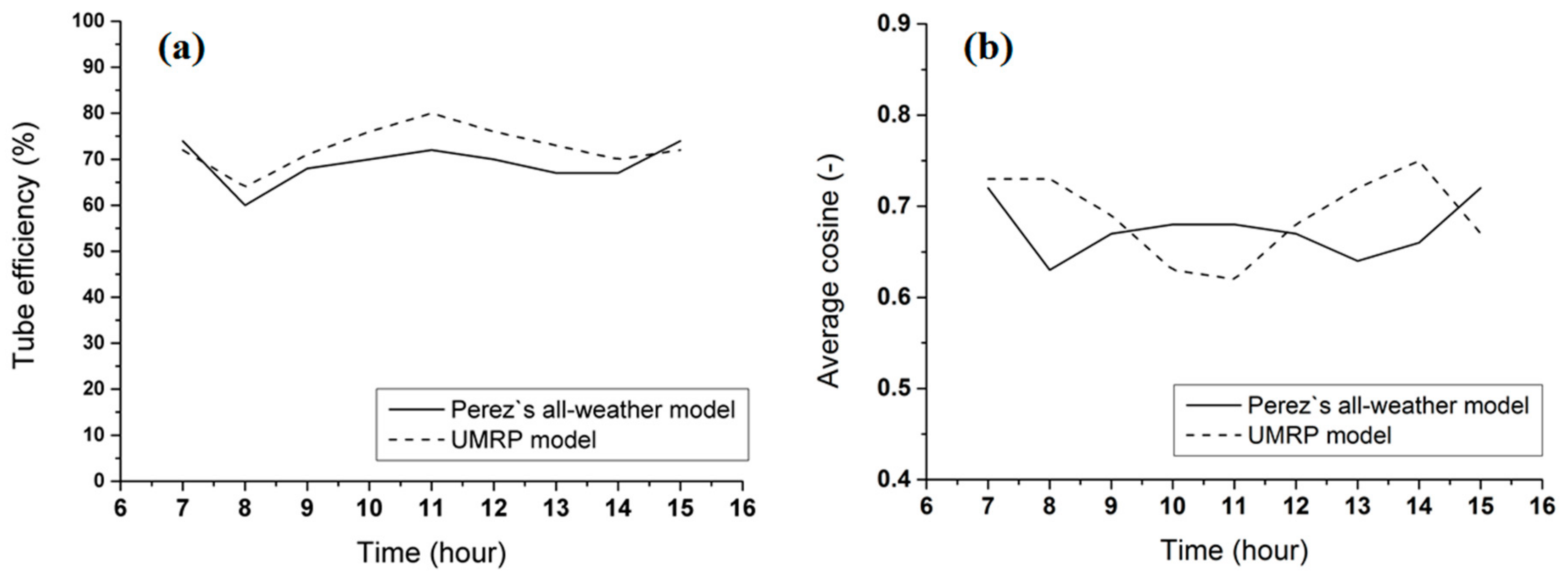
Although the positions of the clouds constantly change, the LTE computed from Perez’s model of a homogeneous sky was found to coincide with more accurate UMRP computations (see Figure 8a, Figure 9a, Figure 10a, Figure 11a and Figure 12a). The largest differences between the LTE data (up to 10%) are found in the winter months and are most likely due to the prevalence of low sun elevations. In general, Perez’s all-weather model underestimates LTE, but the LTEs predicted from both models tend to have the same patterns. The light tube efficiency is a non-directional quantity and only expresses the fraction of exterior light used for the illumination of interior spaces. The light guide harvests light from all directions, so it is not a surprise that the integral of the sky luminance over the definition domain of the zenith angles and azimuth angles averages all imperfections and efficiently suppresses the contribution from local luminance peaks.

However, the average cosine encapsulates the information on preferred directions, thus implying the combination of the LTE and <cos> is a preferred concept to characterize the light guides. This approach is advantageous as <cos> is also a single scalar value, so simple two-valued records are sufficient to distinguish between two skies that do not differ in CF (or $\epsilon$), but produce different illuminance patterns due to different cloud configurations. In principle, Perez’s model is unable to mimic a large variability of <cos>, therefore the differences between the homogeneous, all-weather model and exact UMRP computations can be large (as shown in Figure 8b, Figure 9b, Figure 10b, Figure 11b and Figure 12b). The consequences are marginal for the cloudless or overcast skies, but may be important for skies with several discrete clouds. White clouds can reflect large portions of sunbeams if they appear opposite the sun in the sky, but the same clouds act as dark attenuators when drifting around the sun. These effects cannot be simulated by a model of a homogeneous sky whatever level of complexity it has.

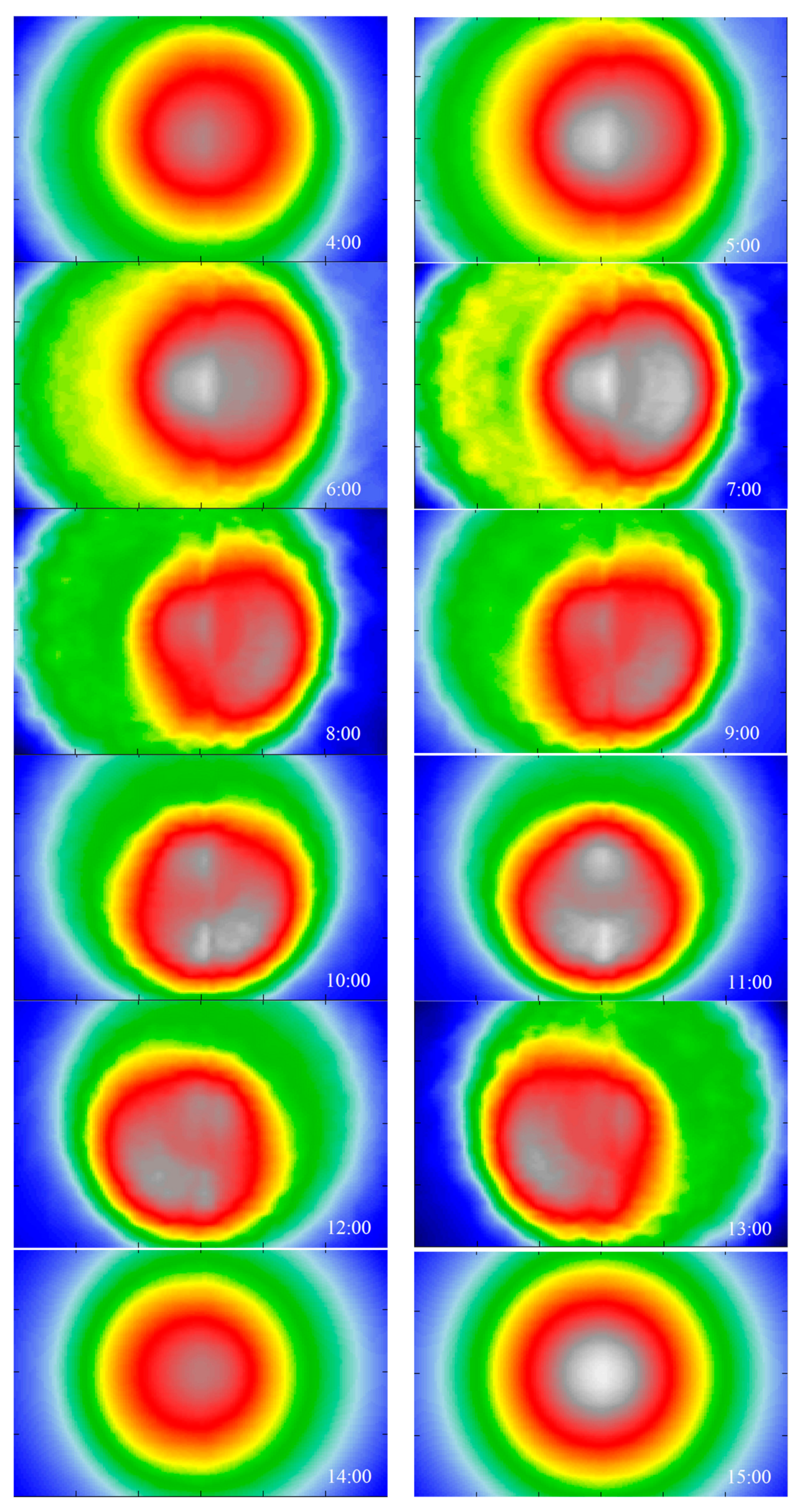
The cloud-initiated distortion and ripple structure of sky luminance patterns can be decisive in shaping the illuminance distribution in room interiors. For this reason we have analyzed in detail the work plane illuminance computed for data collected in 14 June. We have considered room dimensions of 6 m × 4 m, while the axis of the tubular light guide crosses the work plane in its center. The separation distance between the plane of the projection and room ceiling is 3 m. The illuminance distributions computed from the UMRP can show the azimuthal asymmetry because clouds can change the <cos> steeply through amplification of the luminous flux from some part of the sky, so the luminance appears intensified in specific directions. The irregularities observed in Figure 13 disappear when the work plane illuminance is simulated using an all-weather model (see Figure 14). The asymmetry with some plots is only due to the sun position, but no effects from the random cloud arrangement are identified in Figure 14. We can conclude that the use of the homogeneous skies in modeling the light field below the light guide can result in inaccurate estimates of daylight availability in interiors, while having impacts on visual comfort and lighting quality (especially in the core of the buildings).

5. Conclusions

Daylight/sunlight modeling is needed in diverse renewable energy applications from PV, through solar concentrators to daylight harvesting, including the illumination of interior spaces. The latter is important to evaluate the potential of using natural daylight for electric lighting energy savings in buildings. The system of the hollow light pipes is a useful concept to deliver a considerable portion of daylight to interiors. Correct predictions of daylight illuminance levels under different meteorological conditions can be decisive in designing electric illumination systems for various building zones. However, most of the models currently in use are based on a simple concept of the homogeneous skies that on one hand allow for rapid numerical modeling, but on the other hand cannot mimic the real sky states that occur in nature, especially under partly cloudy conditions. Isolated clouds reflect sunlight and also diffuse light in a complex manner, while making the sky luminance a non-monotonic function of the zenith and azimuth angles. Computers are now efficient enough to be used to model sky luminance under unstable broken cloud arrays, so there is no real reason for relying on oversimplified empirical tools.

We have developed a new solution that encapsulates the functionality of the UniSky simulator for computing the sky luminance distribution under the arbitrary cloud coverage and the HOLIGILM tool for obtaining the light field below a hollow tubular light guide. In synergy, these tools represent a unique concept for a fast and accurate prediction of daylight illuminance conditions in building interiors. This new solution allows not only for random cloud sizes and distributions in the sky, but also for modeling cloud arrays drifting from or to a specific direction as observed in many situations. This way the availability of luminous energy can be computed in any site, under any exterior conditions and for any modeling domain. The demonstration is made for a hollow light pipe in order to avoid unwanted (parasitic) effects from pipe bends. However, the computational concept proposed in this paper is not limited to only straight pipes, but is applicable to arbitrary geometries. The UniSky simulator is able to generate the light field that is the input to any light-guide integrator. UniSky Simulator also allows to separate the contribution from the clouds, haze, or air pollution by performing the computations for clean atmosphere first, then for a turbid atmosphere, and then for a specific cloud arrangement, while holding all other parameters constant. Since the configurations differ only in the properties we have added, the relative contribution of the clouds can be obtained from a comparison of the illuminance distributions for the respective cloud model and cloud-free model. This way we can distinguish the effects from the air pollution, haze, or the purely cloudy day.

We have shown that the models of homogeneous skies are successful in the prediction of the light guide efficiency even under partly cloudy conditions, but fail in reproducing the angular distribution of luminous energy in the room interiors. This is because the luminous efficiency is derived from the luminous fluxes at the top and bottom interfaces of a light guide. However, the peak luminance values that appear due to isolated bright clouds or any other imperfections are efficiently suppressed in the process of integration, so there is no reason to suppose that the light-guide efficiency derived from the homogeneous models will deviate much from that computed from an exact sky-luminance model. On the other hand, the cloud arrangement can have a large impact on the directionality of light beams below a light-pipe, and thus on the illuminance patterns as well. Although determined within an acceptable error tolerance the light-pipe efficiency derived from an idealized model is not a guarantee of correct assessment of daylighting quality in the interiors. This is a challenge for engineers who model daylighting and design renewable energy systems to incorporate this concept using large computational tools, while taking advantage of highly accurate numerical predictions. Our tool allows for a systematic assessment of different designs of illumination systems respecting the typical instability of sky states. The targeted computations can also help to propose optimum energy savings solutions depending on room orientations.