A Stratigraphic Prediction Method Based on Machine Learning

Abstract

Simulation of a geostratigraphic unit is of vital importance for the study of geoinformatics, as well as geoengineering planning and design. A traditional method depends on the guidance of expert experience, which is subjective and limited, thereby making the effective evaluation of a stratum simulation quite impossible. To solve this problem, this study proposes a machine learning method for a geostratigraphic series simulation. On the basis of a recurrent neural network, a sequence model of the stratum type and a sequence model of the stratum thickness is successively established. The performance of the model is improved in combination with expert-driven learning. Finally, a machine learning model is established for a geostratigraphic series simulation, and a three-dimensional (3D) geological modeling evaluation method is proposed which considers the stratum type and thickness. The results show that we can use machine learning in the simulation of a series. The series model based on machine learning can describe the real situation at wells, and it is a complimentary tool to the traditional 3D geological model. The prediction ability of the model is improved to a certain extent by including expert-driven learning. This study provides a novel approach for the simulation and prediction of a series by 3D geological modeling.

1. Introduction

A geostratigraphic structure is the result of multiple factors in the course of the evolution of Earth’s history, forming a complex morphology and irregular distribution. Geological bodies have spatially successive relationships, thus forming a series of strata with different lateral extensions and thicknesses. A geostratigraphic series is spatially uncertain due to the variations in sequence and the number and thickness of the stratum layers. Within the rock-soil mass extending from the top of the bedrock (referring to lithified rock that underlies unconsolidated surface sediments, conglomerates or regolith) to the surface, only one layer or dozens of layers can be present. There can be a few layers, and each can be different. At the same time, the thickness of the strata also varies considerably, from tens of centimeters to hundreds of meters. Different geotechnical bodies have different physical, chemical, and mechanical properties, and weak stratum conditions directly threaten the safety of engineering construction and operation. A geostratigraphic series model with high reliability is helpful to understand the geological conditions of a construction area, providing far-reaching practical guidance for site planning and selection, engineering construction, environmental assessment, cost savings, and operational risk reduction. Therefore, building a series model and accurately describing the spatial distribution of strata have become important topics in the field of geology and engineering geology.

To understand the geological structure, many techniques and methods have been developed to describe, simulate, and model strata [1,2,3,4,5,6]. With the introduction of the Glass Earth [7] concept and geological data, interdisciplinary theoretical integration and application research is being carried out. The most representative traditional method of simulating the stratum structure is three-dimensional (3D) geological modeling, such as that with the B-rep model [8], octree model [9], tri-prism model [10] and geochron concepts [11,12,13,14]. However, the traditional method relies on the guidance of expert knowledge and experience in the selection of assumptions, parameters, and data interpolation methods, which are subjective and limited [15]. Assumptions about the borehole data distribution must be made, and it is difficult to effectively evaluate the stratum simulation results.

Machine learning [16,17,18] has been widely used in various fields of geology. The machine learning method does not make too many assumptions about the data but selects a model according to the data characteristics. Then, the machine learning method divides the data into a training set and a test set and constantly adjusts the parameters to obtain better accuracy. Machine learning is more concerned with the predictive power of models [19]. In the fields of geology and engineering, there have been numerous research and application examples in different fields [20,21,22,23,24,25]. Rodriguez-Galiano et al. conducted a study on mineral exploration based on a decision tree [26]. Porwal et al. used radial function and neural network to evaluate potential maps in mineral exploration [27]. Zhang studied the relationships between chemical elements and magmatite and between the sedimentary rock lithology and sedimentary rock minerals by using a multilayer perceptron and back propagation (BP) neural network [28]. Zhang et al. predicted karst collapse based on the Gaussian process [29]. Chaki et al. carried out an inversion of reservoir parameters by combining well logging and seismic data [30]. Gaurav combined machine learning, pattern recognition, and multivariate geostatistics to estimate the final recoverable shale gas volume [31]. Sha et al. used a convolutional neural network to characterize unfavorable geological bodies and surface issues, etc. [32]. Generally, machine learning research on stratum distributions based on drilling data is in its infancy.

To solve the above problems, this study explores the feasibility and reliability of machine learning through the simulation of a geostratigraphic series and proposes a machine learning geostratigraphic series simulation method. This method does not rely on subjective factors, and it is based on the principle of a recurrent neural network [33,34] to establish a stratum simulation model. This method can determine the stratum information accurately. The predictive power of machine learning models is examined with expert-driven mechanism based on supervisory learning [35]. Compared with the traditional 3D geological modeling method, this study shows that the proposed method can better describe the real situation. This study provides a novel approach for the simulation and prediction of a geostratigraphic series. This work has far-reaching practical significance for the accurate description of the spatial distribution of lithologic features and guidance of site selection, engineering construction, and environmental assessment.

2. Geostratigraphic Series Simulation Method Based on Machine Learning

2.1. Geostratigraphic Series

A sequence refers to a series of data of a system at a specific sampling interval. In reality, sequences are a very common form of data. For example, strata have a certain thickness, and a certain stratum may be distributed throughout the whole field or only locally (namely, the stratum division). Stratum information can be interpreted as a sequence. Therefore, the strata can be regarded as a vertically oriented spatial sequence, as shown in Figure 1. The simulation of a geostratigraphic series is based on the learning results of borehole data to predict the geostratigraphic series at any point in the study area, including the stratum type and thickness of each layer in the sequence.

2.2. Stratum Data Reconstruction Schemes Based on Machine Learning

Drilling data reconstruction schemes based on machine learning include data normalization, data segmentation, data filling, and data coding.

2.2.1. Stratum Data Normalization

Data normalization refers to the process of compressing data into a small interval, and the interval is usually taken as [0,1] or [−1,1]. Data normalization is essentially a linear transformation. Data normalization does not change the variation suppress and sequence of the data. There are many common means of data normalization, such as linear normalization, and inverse cotangent normalization. In this study, the most common method of linear normalization is adopted. For any data point, the program determines the spatial coordinates and the maximum and minimum values (X_max and X_min, respectively) of the stratum thickness after traversing all the borehole data. The above linear normalization is applied by using Equation (1):

X = (X − X_min)/(X_max − X_min)

(1)

where X is the result of normalization.

2.2.2. Drilling Data Segmentation and Equalization

Machine learning is used to ensure that the designed model achieves good prediction results in both the training set and the test set. Therefore, before machine learning, the original drilling data must be divided into training data and test data. This process is called data segmentation. To ensure the effectiveness of machine learning, randomness and uniformity of the data distribution should be ensured during sampling of the training data and test data.

To ensure the effectiveness of the training data, we adopt a random replication strategy for small samples. We randomly select data from boreholes with different numbers of geological layers to improve the replication effect. This method is used to comprehensively study data with different characteristics, improve the prediction ability of a model for different numbers of geological layers, increase the number of different layers represented by nearby drilling data, and artificially upgrade the training sample data at the equilibrium level. This approach of artificially replicating small data types is known as over sampling [36].

2.2.3. Geostratigraphic Series Filling

When a recurrent neural network (RNN) is used to process sequential problems, input data are received at every moment, and output is produced after the hidden layer has finished processing the data. Therefore, the input and output of an RNN are equal in length, and it is difficult to process input data of different lengths at the same time. In drilling data, the number of layers in each borehole varies, and the geostratigraphic series is nonuniform. Therefore, the use of an RNN for batch training using stratum data requires filling at the tail of the geostratigraphic series without changing the original sequence of the geostratigraphic series and extending all geostratigraphic series to the same length [37]. Before training, in addition to adding a start of sequence (SOS) to the geostratigraphic series, an end of sequence (EOS) must be added to the geostratigraphic series. For each training set, the sampling process stops when the termination marker appears in the equal length geostratigraphic series output of the RNN. As two virtual stratum types, the initiation and termination markers participate in the RNN training process via the input and output. The initiation markers represent the beginning of geostratigraphic series prediction, while the termination markers represent the end of the series prediction. The introduction of termination markers teaches the RNN model to predict when a sequence will end and overcomes the shortcomings of processing unequally long sequences by the RNN. In addition, the RNN model can conduct geostratigraphic series simulations with different numbers of layers at any location in the research area.

2.2.4. Stratum Coding Based on One-Hot Encoding

In machine learning tasks, data characteristics are not always continuous values, such as coordinates. One-hot encoding is a data processing method used to address discrete features. In geology, stratum types are finite and countable, regardless of the criteria used to divide the strata. Therefore, the set of geostratigraphic series elements is determined after crossing all the borehole data, in addition to obtaining the maximum value of each feature and the number of layers. To facilitate the search and mathematical representation, in this study, each stratum is represented by a unique digital identification [38].

2.3. Geostratigraphic Series Simulation Based on a Recurrent Neural Network

2.3.1. Establishment of the Sequence Model of the Stratum Type

The model in geostratigraphic series prediction uses the RNN as the core of the neural network. The structure is shown in Figure 2. In the machine learning tasks, the input data are coordinated in a stratum, while the output result is the simulation result of the stratum type model corresponding to the given coordinates. Since the RNN does not have a state hidden from the previous moment at the current moment, it is necessary to assign the initial state of the hidden layer neurons in the RNN before each training run. The input coordinates are the common attributes of all the strata in a geostratigraphic series, and it guides the whole process of RNN simulation of the geostratigraphic series. Therefore, the assignment process establishes the correlation between the input coordinates and RNN, guiding the geostratigraphic series simulation from the beginning. The content of the assignment is determined by the input information. After the input layer receives the coordinates of the borehole and the basic elevation information, the coordinate input information is increased from the original three dimensions to the number of dimensions equal to the number of neurons. It serves as the initial state of the hidden layer neurons in the RNN.

At each moment, the RNN receives input of the neuron state and stratum information from the previous moment, and outputs the judgement of the stratum type through hidden layer calculations. By introducing an n-dimensional correct value vector, each item in the weight vector represents the possibility of a certain stratum. The larger the value is, the higher the probability of a certain stratum. Thus, the most likely stratum is the predicted value at that moment. Repeating the above process and removing the termination marker in the output, we can obtain the model’s simulation results for the input coordinate information of the geostratigraphic series.

2.3.2. Establishment of the Series Model of the Stratum Thickness

Sequence-to-sequence (or seq2seq) learning has been widely used in the processing of machine translation and speech recognition, also known as the encoder-decoder network. It maps sequences as input to output sequences through deep neural networks. The seq2seq model is shown in Figure 3. This process includes two steps, input encoding and output decoding and these two links are handled by the encoder and decoder, respectively. The encoder is responsible for converting a variable-length input series into a fixed-length vector. This fixed-length vector contains information about the input series. The encoder is responsible for decoding this fixed-length vector and generating a variable-length output series according to the information content the vector represents.

In contrast to the traditional RNN, the seq2seq architecture does not require input and generates output at every moment. Instead, the algorithm converts the input series of the stratum types into a vector with the help of the encoder, and then outputs the results through the decoder. In other words, seq2seq carries more information when making predictions than the traditional RNN and infers the output content based on the input series as a whole.

In this study, two RNNs are used as the encoder and decoder which are connected to each other. Seq2seq is now widely used to process machine translation and speech recognition problems, thus, we apply it to the layer thickness recognition problem, that is to say, given the geostratigraphic series x = [x1, x2, x3, …,xn], an equal-length thickness sequence d = [d1, d2, d3, …,dn] is generated. N is the length of the sequence (i.e., the total number of strata at that point). The encoder receives the type information of the current stratum at each moment, n times in total. After the input has been completely received, the hidden state, at the last moment of the encoder, is taken as the initial state to guide the decoder. Then, the decoder outputs the thickness of each layer step-by-step. The above process and model structure are shown in Figure 4.

2.3.3. Establishment of the Geostratigraphic Series Modeling

The stratum thickness model uses real stratum type data in the training process. In practice, the real stratum type is unknown, and the output sequence of the stratum type model should be used as the judgement basis. The output of the stratum type model is connected with the encoder of the layer thickness model. We can obtain a complete geostratigraphic series model. The simulation sequence of the layer thickness is shown in Figure 5 and Figure 6.

2.4. Evaluation Method of Stratum Type Series Simulation

The stratum accuracy, the series edit distance, and the geostratigraphic series similarity based on the edit distance are used to evaluate the simulation performance of the series models of the stratum type.

The stratum accuracy is the simplest evaluation index. By comparing elements at corresponding positions of the simulated sequence and the real geostratigraphic series, the proportion of the same number of strata in the total number of strata was calculated by Equation (2):

$$\frac{\mathrm{Correct}\mathrm{stratum}\mathrm{number}}{\mathrm{Total}\mathrm{formation}\mathrm{number}\mathrm{of}\mathrm{test}\mathrm{data}}$$

(2)

The edit distance is a standard that is used to measure the similarity of series. The edit distance represents the minimum number of edit operations required for one series to be converted into another series after insertion, deletion, and replacement. The smaller the edit distance between the two series, the more similar the two series are. Since the length of the series for edit distance alignment is different, the longer series has a notably higher similarity when editing two series with the same distance. To better describe the closeness of series, the following Equation (3) is used in the calculation of the similarity of series:

$$\mathrm{L}\left(\mathrm{S},\mathrm{T}\right)=1-\frac{\mathrm{D}\left(\mathrm{S},\mathrm{T}\right)}{\max \left(\left|S\right|, \left|T\right|\right)}$$

(3)

where D(S, T) represents the edit distance between series S and T.

There is no exact equation for calculating D(S, T). Its calculation examples are as follows:

Suppose there are two geostratigraphic series, t1 = [silt, fine sand, silt, clay, silt, clay] and t2 = [miscellaneous fill, sand, fine sand, silt, clay]. In order to convert t1 to t2, the implementation process of the minimum operation times is as follows:

• Replace the first “silt” with “sand”;
• Insert “miscellaneous fill” at the beginning of t1;
• Remove the last “clay”;
• Delete the final “silt”.

Throughout the above four steps to replace, delete, and insert operations, the geostratigraphic series t1 changed to series t2. Thus, the two geostratigraphic series of edit distance D(S, T) is 4.

Although the transition from one series to another through several insertions, deletions, and substitutions has many possibilities, the editing distance D(S, T) between the two series is always unique.

3. Results and Discussions

3.1. Study of the Regional Geology and Data Reconstruction Schemes

The research area is located in a city in eastern China with a plain topography. The soil in the study area is mainly composed of sandy soil, cohesive soil, and silty soil. The local strata are silt and silty soil. The research data come from the city’s geological survey work. There is a total of 1386 borehole datasets, and all the boreholes terminate on the bedrock surface. A total of 13 stratum types were determined. These boreholes are nonuniformly distributed in an area of 3882 square kilometers, as shown in Figure 7.

Using the reconstruction scheme of the stratum data proposed in this study, the drilling data are reconstructed. The specific operation process is as follows:

1. Data normalization: In this study, the borehole data are used and the x coordinates, y coordinates, hole elevation, and stratum thickness are continuous values. After reviewing all the borehole data, it is found that the coordinates of the borehole data used the Xi’an 80 coordinate system, and their value reaches the millions, while the elevation of the orifice and the thickness of the strata are only within 100 m. The difference between each characteristic is large and can be up to tens of thousands. To ensuring the same dimension, the above borehole data characteristics are compressed into the interval of [0,1] by linear normalization processing.

2. Drilling data segmentation and equalization: In this study, the training data and test data are selected randomly according to the ratio of 4:1 among all drilling points, and the data are balanced according to the number of layers. The spatial positions of the training data and test data are shown in Figure 8.

Figure 8 shows the location distributions of the training data and test data in the study area after the original drilling data are segmented into training data and test data, where the red symbols represent the training data, and the green symbols represent the test data. The positions, plotting scale, and geographic coordinates in Figure 8 are the same as in Figure 7.

3. Stratum coding: According to the statistics, the borehole stratum data used, in this study, contain a total of 13 types of strata and 15 types of initiation and termination markers artificially introduced in the subsequent geostratigraphic series. The numbers zero to 14 were assigned, and vectorization was carried out by one-hot encoding. The number and coding vectors of the stratum types are shown in

Table 1. Strata numbers and one-hot vectors.

Stratum Types	Number	Coding Vector
clay	0	(1, 0, 0, 0, 0, 0, 0, 0, 0, 0, 0, 0, 0, 0, 0)
silt	1	(0, 1, 0, 0, 0, 0, 0, 0, 0, 0, 0, 0, 0, 0, 0)
plain fill	2	(0, 0, 1, 0, 0, 0, 0, 0, 0, 0, 0, 0, 0, 0, 0)
miscellaneous fill	3	(0, 0, 0, 1, 0, 0, 0, 0, 0, 0, 0, 0, 0, 0, 0)
silty sand	4	(0, 0, 0, 0, 1, 0, 0, 0, 0, 0, 0, 0, 0, 0, 0)
silty clay	5	(0, 0, 0, 0, 0, 1, 0, 0, 0, 0, 0, 0, 0, 0, 0)
mucky soil	6	(0, 0, 0, 0, 0, 0, 1, 0, 0, 0, 0, 0, 0, 0, 0)
mucky clay	7	(0, 0, 0, 0, 0, 0, 0, 1, 0, 0, 0, 0, 0, 0, 0)
old city fill	8	(0, 0, 0, 0, 0, 0, 0, 0, 1, 0, 0, 0, 0, 0, 0)
clay sand inclusion	9	(0, 0, 0, 0, 0, 0, 0, 0, 0, 1, 0, 0, 0, 0, 0)
mud	10	(0, 0, 0, 0, 0, 0, 0, 0, 0, 0, 1, 0, 0, 0, 0)
medium sand	11	(0, 0, 0, 0, 0, 0, 0, 0, 0, 0, 0, 1, 0, 0, 0)
intermediate fine sand	12	(0, 0, 0, 0, 0, 0, 0, 0, 0, 0, 0, 0, 1, 0, 0)
start mark	13	(0, 0, 0, 0, 0, 0, 0, 0, 0, 0, 0, 0, 0, 1, 0)
end mark	14	(0, 0, 0, 0, 0, 0, 0, 0, 0, 0, 0, 0, 0, 0, 1)

.

4. Geostratigraphic series filling: According to the statistics, the maximum number of strata in the study data is 10. Therefore, the filling length of the geostratigraphic series should be larger than 10 layers. For simplicity, the termination marker is used here to fill all geostratigraphic series to the 11th layer. Suppose that all stratum types of a borehole are clay, silt, silt sand, clay, and mucky clay, and the corresponding number vector is expressed as (0,1,4,0,7). The termination marker denoted by the number 14 is repeatedly added at the end of the vector until the length of the numbered vector is 11. Finally, the geostratigraphic series data input of the machine learning model is obtained by replacing each item in the numbered vector with the corresponding one-hot encoding vector.

3.2. Machine Learning Simulation Result Analysis

We have implemented the proposed algorithms written by Python software in the computer. Part of the algorithm code is as follows:

• class CrossLoss(nn.Module):
• def __init__(self,ignore_index = 0):
• super(CrossLoss, self).__init__()
• self.ignore_index = ignore_index
• self.criterion = nn.CrossEntropyLoss(ignore_index = 0)
• def forward(self, input, target):
• ind = (target ! = self.ignore_index).float()
• num_all = torch.sum(ind).data[0]
• #print(target)
• size0 = target.size(0)
• size1 = target.size(1)
• temp = target.cpu().data
• for i in range(size0):
• for j in range(size1):
• temp[i,j] = depthLabel(temp[i,j])
• pred = torch.mul(input,ind).long()
• temp = temp.long()
• loss = self.criterion(pred, temp)
• return loss, num_all

As the procedure may be further commercialized, it is not suitable to make it all public for the time being.

Information about the algorithm’s computer performance is as follows:

• CPU: Intel Core i7-4790k @ 4.00GHz quad-core;
• Memory: 32 GB;
• VGA card: Nvidia GeForce GTX 770(2GB).

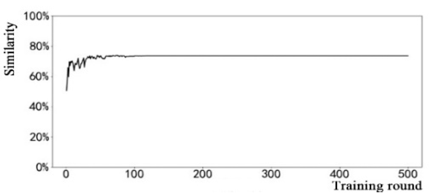
3.2.1. Training and Verification of the Stratum Type Series Model

(1) Model Training

The cross-entropy loss function is used to describe the performance of the model in the training process. Figure 9 shows that as the number of training rounds increases, the loss value decreases continuously. However, the gradient of the loss curve begins to decrease after several cycles, and the amplitude of change gradually decreases. The final loss value fluctuates in a small range and tends to be stable.

The model has completed most of its loss reduction after 50 training rounds, as shown in Figure 10. After 50 rounds, the loss function tends to be stable, and the model is slowly learning from the training data. The specific decline in the loss function is listed in

Table 2. Statistical table of the loss decline.

Round Number	50	500
Loss value	0.483226	0.374167
Cumulative decline	0.327009	0.436068
Cumulative decline	40.36%	53.82%

.

(2) Model Test

The trained and finally stable model was tested, and the coordinate information of the test borehole data was inputted successively. The position of the termination marker in the simulated stratum type sequence output by the model was searched and intercepted. All the elements before the first termination marker were taken as the stratum prediction series. By comparing the predicted value with the real value one-to-one, the single-layer accuracy of the geostratigraphic series is tested. Then the similarity between the prediction sequence and the real geostratigraphic series is evaluated by using the edit distance algorithm.

The accuracy of stratum type simulation varies with the training round, as shown in Figure 11. Figure 11 shows that as the number of training rounds increases, the overall prediction ability of the model continues to improve, and the accuracy of the stratum type and geostratigraphic series prediction is rapidly improved. The accuracy of the final stratum type prediction was stable at 59.86%. As the loss function curve changes, the accuracy curve increases gradually. The accuracy achieved in the first 50 rounds is almost the same as the final accuracy.

The prediction of a single stratum is the first step in establishing a spatial stratum distribution model. In addition to the accurate prediction of a single stratum, it is of greater concern whether the model can make an accurate overall prediction of the geostratigraphic series in the study area. Then, the edit distance algorithm is used to evaluate the similarity between the simulated sequence and the real geostratigraphic series. If the edit distance between the prediction sequence and the real geostratigraphic series is larger than one, the prediction failed and will not be considered. The edit distance changes are shown in Figure 12.

In Figure 12, the lower curve indicates that the edit distance is zero, i.e., the proportion of the number of boreholes in the predicted result in the test set is exactly equal to the real result. The above curve indicates the proportion of the number of boreholes within an edit distance of one, i.e., the model makes no more than one wrong prediction in the whole sequence prediction process. The predicted sequence can be converted into a real stratum sequence by a single insertion, replacement, or deletion operation. In the end, the former curve converges to 35.2%, while the latter curve converges to 74%.

Because the number of layers is different, it is difficult to accurately describe the similarity between the predicted series and the real result by applying the edit distance alone. Therefore, the similarity calculation equation based on the edit distance is adopted. The variation curve of the predicted series similarity with the number of training rounds is shown in Figure 13.

In Figure 13, with an increase in training rounds, the overall prediction ability of the model is continuously improved, and the average similarity curve between the predicted series and the actual geostratigraphic series also gradually increases and finally converges to 70.9%. This result shows that model accuracy continuously improves with increasing training rounds in the learning process and gradually establishes the correlation between the elevation information and the geostratigraphic series in the study area.

(3) Testing the Effect of Expert-Driven Learning

To improve the learning performance of the RNN and test the effect of expert-driven learning, this study conducted the training and testing of the expert-driven model based on supervisory learning in accordance with four ratios using the same dataset. The four expert ratios are 1/3, 1/2, 2/3 and 1, i.e., expert-driven learning is carried out once every three rounds, once every two rounds, and twice every three rounds, and the entire training process is conducted in the form of expert-driven learning.

Figure 14, Figure 15, Figure 16 and Figure 17 show the loss function curves of expert-driven learning using different factors. Since the model is based on the prediction results of both expert-driven learning and non-expert-driven learning, the loss function is banded in the first three figures. The model obtained a higher descent gradient under the guidance of correct monitoring signals as compared with the ordinary RNN model. The larger the proportion of expert-driven learning in the learning process is, the higher the rate of loss reduction. When expert-driven learning is completely adopted, the model loss function curve decreases the fastest. Almost all of the gradient descent is completed within the first 50 training rounds.

The single-stratum accuracy rate curve in each test round is shown in Figure 18, Figure 19, Figure 20 and Figure 21.

The accuracy of the model simulation results under different tutor ratios is shown in

Table 3. Stratum type accuracy under different expert ratios.

Expert Ratio	0	1/3	1/2	2/3	1
Maximum value	61.42%	63.83%	64.82%	63.40%	64.82%
Steady value	59.86%	60.00%	62.41%	61.13%	60.42%

below.

Figure 22, Figure 23, Figure 24 and Figure 25 show the proportion of the drilling data with edit distances of zero and one in the total test data between the prediction series of the model and the real geostratigraphic series. Detailed statistics are shown in

Table 4. Statistical results of the edit distance under the different expert ratios.

Expert Ratio		0	1/3	1/2	2/3	1
Edit Distance = 0	Maximum value	37.2%	39.6%	39.2%	39.6%	36.4%
	Steady value	35.2%	38%	38.4%	38.4%	35.6%
Edit Distance <= 1	Maximum value	76%	77.2%	76.4%	77.2%	76.4%
	Steady value	74%	75.6%	75.6%	75.6%	73.6%

.

The similarity curves between the prediction series of the model and the real geostratigraphic series under different expert ratios is shown in Figure 26, Figure 27, Figure 28 and Figure 29.

The statistics of series similarity under different expert ratios are shown in

Table 5. Statistical results of the series similarity.

Expert Ratio	0	1/3	1/2	2/3	1
Maximum value	71.85%	73.60%	73.95%	73.98%	72.51%
Steady value	70.91%	72.64%	73.57%	73.09%	71.68%

.

It can be seen that adopting the expert-driven learning mechanism is helpful to improve the performance of test models for stratum type series simulation based on machine learning, as shown in Table 5. However, the amplitude of the improvement effect is not significant. The expert-driven model can accelerate the convergence of the learning curve, and the higher the expert ratio is, the faster the model will reach stability. From the highest and stable values of the various indicators in the different models, it is not the rule that the higher the expert ratio is, the better the effect will be. The ultimate performance of full expert-driven learning was only slightly better than that of the RNN model. The best results were obtained by using a partial expert-driven learning strategy model.

3.2.2. Training and Verification of the Stratum Thickness Series Model

(1) Layer Thickness Simulation Based on Multi-Category Classification

The layer thickness of the study area is divided into six stratum thickness intervals as follows: within 3 m, 3 m to 5 m, 5 m to 10 m, 10 m to 20 m, 20 m to 30 m, and above 30 m. Stratum thickness series simulation based on multi-category classification also needs to be numbered and coded for the different stratum thicknesses, as shown in

Table 6. Code of the layer thickness type.

Stratum Thickness Interval	Layer Thickness Type Coding Number	Coded Vector
<3 m	0	[1, 0, 0, 0, 0, 0, 0]
3–5 m	1	[0, 1, 0, 0, 0, 0, 0]
5–10 m	2	[0, 0, 1, 0, 0, 0, 0]
10–20 m	3	[0, 0, 0, 1, 0, 0, 0]
20–30 m	4	[0, 0, 0, 0, 1, 0, 0]
>30 m	5	[0, 0, 0, 0, 0, 1, 0]
initiation mark	6	[0, 0, 0, 0, 0, 0, 1]

.

Before the output of the model is generated, the encoder has received a complete series of stratum types, that is, the total number of stratum layers at the prediction point is known. Therefore, there is no need to add a termination marker for the layer thickness interval. Only an initiation mark is introduced as the starting point of the decoder’s simulated layer thickness sequence. After all outputs of the model are completed, a series equal to the number of layers is intercepted as the prediction sequence of the layer thickness.

(2) Model Training and Testing

The stratum thickness series model adopts the seq2seq architecture and uses the drilling data in the training set for training. To accurately reflect the actual performance of the model, the highest accuracy and average accuracy of the model in the test set were compared. After each round of training, the model was tested, and the test results were recorded. After training 500 rounds, the loss curve of the model is shown in Figure 30, and the changes in prediction accuracy are shown in Figure 31. As the number of training rounds increases, the prediction performance of the model increases slowly and finally converges to 63.53%.

(3) Testing the Effect of Expert-Driven Learning

To further improve the accuracy of the model and improve the prediction ability of the model for the stratum thickness category, this section conducts expert-driven model based on supervisory learning in different proportions and compares the learning effect to determine the model with the highest accuracy and the greatest prediction ability. In this section, the expert ratios adopted by the seq2seq model in the learning process are 1/3, 1/2, 2/3, and 1. The accuracy performance of the different models in test data is provided in

Table 7. Prediction accuracy of the layer thickness.

Expert Ratio	0	1/3	1/2	2/3	1
Maximum value	65.07%	73.05%	80.08%	75.60%	70.07%
Steady value	63.53%	70.07%	75.05%	72.62%	67.94%

.

Table 7 shows the highest value of the results achieved in the test data and the final stable value after convergence, based on the different expert ratios. As we can see from the test results, with the increase in the proportion of expert-driven learning, the accuracy of the model in terms of the test data first increases and then decreases. In addition, the models that do not adopt expert-driven learning and completely adopt expert-driven learning do not achieve the highest accuracy. Clearly, the relationship between the expert ratio and the prediction accuracy rate is not simply a positive correlation. The loss function of 50% expert-driven learning and the training process is shown in Figure 32. When 50% expert-driven learning is applied, the stable value of the layer thickness prediction accuracy is 75.05%, and the highest value is 80.08%, which is the best model performance in the test set, as shown in Figure 33. At this point, the prediction ability of the model for unknown data is the greatest, which is consistent with the experience with the stratum type identification model. Therefore, expert-driven learning can improve the prediction ability of the model and accelerate convergence, but it is not the rule that the higher the expert ratio is, the better the performance of the model.

The final results show that the maximum accuracy of the layer thickness model is 80.85% under the 50% expert ratio, which accurately predicts the layer thickness in the test data.

3.2.3. Verification of the Geostratigraphic Series Model

To verify the true prediction ability of the geostratigraphic series model, the stratum data in the test borehole data are used for practical testing, and the differences between the simulated series output by the model and the real geostratigraphic series are compared. Selected examples of the real borehole stratum conditions and prediction results of machine learning are shown in

Table 8. Comparison of the real borehole stratum and machine learning prediction results.

Number	The Real Borehole Strata		Prediction Results of Machine Learning
	Stratum Type Sequence	Stratum Thickness Sequence (m)	Stratum Type Sequence	Stratum Thickness Sequence (m)
1	silt, clay	0.3, 3.9	floury soil, clay, plain fill	within 3 m, within 3 m, 3–5 m
2	clay	2	clay	within 3 m
3	miscellaneous fill	0.6	plain fill	5–10 m
4	plain fill, clay	3.1, 9.8	plain fill, clay	within 3 m, 5–10 m
5	miscellaneous fill, clay, mucky soil, plain fill, clay	1.2, 1.3, 1.5, 2.4, 13.3	miscellaneous fill, plain fill, mucky soil, plain fill, clay	within 3 m, within 3 m, within 3 m, within 3 m, 10–20 m
6	floury soil, silty clay, plain fill, clay, plain fill, clay	1.0, 0.5, 2.5, 1.2, 0.3, 3.6	floury soil, plain fill, clay, plain fill, clay	within 3 m, within 3 m, within 3 m, within 3 m 5–10 m
7	miscellaneous fill, plain fill, clay	0.7, 3.0, 4.5	miscellaneous fill, plain fill, clay	within 3 m, within 3 m, 3–5 m
8	miscellaneous fill, clay	0.6, 4.0	miscellaneous fill	within 3 m
9	miscellaneous fill, plain fill, clay	0.5, 1.0, 11.9	miscellaneous fill, plain fill, clay	within 3 m, within 3 m, 10–20 m
10	miscellaneous fill, clay	1.0, 9.8	miscellaneous fill, clay	within 3 m, 5–10 m
11	miscellaneous fill, silt, plain fill, clay	4.1, 11.2, 7.0, 10.0	miscellaneous fill, plain fill, clay	within 3 m, 10–20 m, 5–10 m
12	floury soil, plain fill, mucky soil, clay	0.5, 6.7, 1.2, 8.6	floury soil, plain fill, plain fill, clay	within 3 m, within 3 m, within 3 m, 5–10 m
13	silt, clay	0.4, 6.6	floury soil, clay	within 3 m, 5–10 m
14	silt, clay	0.4, 10.4	floury soil, clay	within 3 m, 5–10 m
15	miscellaneous fill, silt, plain fill, clay	0.7, 1.9, 3.4, 24.0	miscellaneous fill, floury soil, plain fill, clay	within 3 m, within 3 m, within 3 m, 20–30 m
16	miscellaneous fill soil, plain fill soil, old city miscellaneous fill soil, clay	1.2, 2.6, 6.5, 13.0	miscellaneous fill, floury soil, plain fill, old town fill, clay	within 3 m, within 3 m, within 3 m, 5–10 m, 10–20 m
17	miscellaneous fill soil, plain fill soil, clay	0.5, 2.8, 10.2	miscellaneous fill, plain fill, clay	within 3 m, within 3 m, 10–20 m
18	miscellaneous fill soil, plain fill soil, clay	2.1, 0.8, 12.9	miscellaneous fill, plain fill, clay	within 3 m, within 3 m, 10–20 m,

.

Table 8 shows that by comparing the prediction results of the model with the real borehole data, the machine learning model based on the seq2seq architecture has a high accuracy in stratum type prediction. According to the statistics, in all data of the test set, the machine learning model accurately simulates 62.98% of the stratum types, and the similarity between the simulated sequence and the real stratum sequence is 72.16%. In addition, the accuracy rate of the stratum thickness prediction is 74.04%, which basically realizes the determination of the stratum thickness in the study area, as shown in

Table 9. Statistical results of the geostratigraphic series model simulations.

Stratum Type Accuracy	Average Sequence Similarity	Stratum Thickness Accuracy
62.98%	72.16%	74.04%

.

In conclusion, the machine learning model based on a recurrent neural network can accurately simulate the real stratum situation in the study area, and its feasibility is verified.

3.3. Three-Dimensional Geological Modeling and Testing

3.3.1. Three-Dimensional Geological Modeling

To further test the geostratigraphic series simulation effect based on machine learning, this section compares the geostratigraphic series simulation method based on machine learning with the traditional method based on 3D geological modeling. On the basis of the training data, a 3D geological model of the research area is constructed by using the triangulated irregular network (TIN) 3D geological modeling method [39]. The 3D geological model is consistent with the real strata at the borehole locations, and it can directly show the complex geological structure and the spatial distributions of the rock and soil masses comprehensively.

The main steps for the construction the 3D geological model in this study are as follows:

1. Drilling treatment: According to the geological conditions and drilling stratification data, the strata are classified and integrated, and the strata are preliminarily sorted from top to bottom.

2. Interpolation mesh generation: Using Delaunay’s triangulation and subdivision algorithms, a TIN mesh is generated, as shown in Figure 34.

3. Network refinement: The generated irregular triangular interpolation network is adjusted until the accuracy meets the requirements.

4. Uniform drilling series: All drilling holes are traversed and a uniform geostratigraphic series is established by considering special stratum conditions such as missing data and reversals. Then, according to the unified geostratigraphic series, the original stratification of all borehole data is transformed into a unified stratification of the borehole series, as shown in Figure 35. If a stratum is not included in the original data of the borehole, its layer thickness is set to zero.

5. Spatial interpolation: For each layer of the uniform drilling series, the Kriging method is used to calculate the elevation at the top and bottom of the layer in the interpolation grid. If the elevation of the top layer is the same as that of the bottom layer, this layer does not exist.

6. Stratum construction: If the elevation of the top and bottom of the stratum are different, the top and bottom can be connected with adjacent points to the interpolation point to form a stratum of the 3D model, as shown in Figure 36.

7. Inspection: The generated 3D model is inspected, and the model is adjusted according to experience and geological characteristics.

8. Model generation: A 3D stratum model is rendered, and the redundant parts are removed, while only the research area is maintained.

The method to determine the boundary conditions of the model is as follows: According to boundary on the map of the study area, boundary points are selected at appropriate distances. The boundary points are used as the control points of the estimated stratigraphic boundaries. Then, these control points are connected successively to form a closed polygon. The closed polygon is used as the boundary of the estimated stratum. After determining the estimated stratigraphic boundary, we extended the area of the borehole to the boundary of the estimated stratum and eventually established the entire 3D geological model.

The whole process of 3D geological model modeling, from borehole data processing to the final generation of the model, is shown in Figure 37 below.

Finally, a 3D geological model of the research area is constructed (as shown in Figure 38) and sectioned. The stratum types and series after sectioning are shown in Figure 39, Figure 40 and Figure 41.

3.3.2. Three-Dimensional Geological Model Verification

At the same positions as the data in Section 3.2.3, the borehole coordinate information is input into the 3D geological model. Then the comparison prediction results between the 3D geological model and the real borehole stratum are obtained, as shown in

Table 10. Comparison of the real borehole stratum conditions and 3D geological modeling prediction results.

Number	The Real Borehole Strata		Prediction Results of 3D Geological Modeling
	Stratum Type Sequence	Stratum Thickness Sequence (m)	Stratum Type Sequence	Stratum Thickness Sequence (m)
1	silt, clay	0.3, 3.9	clay, silt	0.3, 3.9
2	clay	2	miscellaneous fill	2.0
3	miscellaneous fill	0.6	miscellaneous fill	0.6
4	plain fill, clay	3.1, 9.8	miscellaneous fill	13.5
5	miscellaneous fill, clay, mucky soil, plain fill, clay	1.2, 1.3, 1.5, 2.4, 13.3	miscellaneous fill, clay, mucky soil, silt	1.2, 1.3, 3.9, 13.3
6	floury soil, silty clay, plain fill, clay, plain fill, clay	1.0, 0.5, 2.5, 1.2, 0.3, 3.6	plain fill, silt clay, silt, clay, silt	1, 0.5, 2.5, 1.2, 3.9
7	miscellaneous fill, plain fill, clay	0.7, 3.0, 4.5	miscellaneous fill, silt	0.7, 8.5
8	miscellaneous fill, clay	0.6, 4.0	miscellaneous fill	4.6
9	miscellaneous fill, plain fill, clay	0.5, 1.0, 11.9	miscellaneous fill, silt	0.5, 0.5
10	miscellaneous fill, clay	1.0, 9.8	miscellaneous fill	12.2
11	miscellaneous fill, silt, plain fill, clay	4.1, 11.2, 7.0, 10.0	miscellaneous fill, silt	2.8, 25.2
12	floury soil, plain fill, mucky soil, clay	0.5, 6.7, 1.2, 8.6	plain fill, silt	0.5, 16.5
13	silt, clay	0.4, 6.6	plain fill	7
14	silt, clay	0.4, 10.4	plain fill	10.9
15	miscellaneous fill, silt, plain fill, clay	0.7, 1.9, 3.4, 24.0	miscellaneous fill, plain fill, silt, silt	0.7, 1.9, 3.4, 24
16	miscellaneous fill soil, plain fill soil, old city miscellaneous fill soil, clay	1.2, 2.6, 6.5, 13.0	miscellaneous fill, plain fill, old city miscellaneous fill soil	1.2, 2.6, 22.5
17	miscellaneous fill soil, plain fill soil, clay	0.5, 2.8, 10.2	miscellaneous fill, plain fill	0.5, 13
18	miscellaneous fill soil, plain fill soil, clay	2.1, 0.8, 12.9	miscellaneous fill, silt, clay	2.1, 0.8, 12.9

.

From Table 10, the 3D geological model performs poorly in terms of the number of layers, stratum type, and sequence similarity, but it can better predict the stratum thickness. When the prediction of the stratum type is accurate, the corresponding thickness prediction is close to the real value.

Some borehole data are randomly selected in the training set, and the borehole coordinate information is input into the 3D geological model to obtain the stratum sequence prediction results of the borehole points. According to the statistics, in all the data of the test set, the 3D geological model accurately simulates 30.78% of the stratum types, and the similarity between the simulated series and the real geostratigraphic series is 32.27%. In addition, the accuracy rate of the stratum thickness is 64.52%, as shown in

Table 11. Statistics of 3D geological model prediction results.

Stratum Type Accuracy	Average Sequence Similarity	Stratum Thickness Accuracy
30.78%	32.27%	64.52%

.

Comparing Table 9 and Table 11, the prediction results histogram of machine learning and 3D geological modeling is obtained in terms of the stratum type, average series similarity, and stratum thickness accuracy, as shown in Figure 42.

Figure 42 shows that there is a certain difference in accuracy between the geostratigraphic series models based on 3D geological modeling and machine learning. Generally, these two methods can describe the real stratum situation well. The model based on machine learning has a good simulation effect in terms of the stratum type, and all its corresponding indexes are superior to those of the traditional 3D geological model. The machine learning model provides stratum information by predicting the layer thicknesses within the strata and it is slightly more accurate than the 3D geological model.

3.4. Evaluation of 3D Geological Modeling Based on the Geostratigraphic Series Model

Considering the actual performance of the machine learning model in the prediction of the stratum type and stratum thickness, this study proposes an evaluation algorithm for a 3D geological model. In the absence of real data guidance, the learning results based on the machine learning model represent the accuracy of geological modeling. For any geostratigraphic series, the reliability evaluation process is described below.

The evaluation objects are divided into a stratum type series and stratum thickness series. The geostratigraphic series model generates output in the same position, including stratum type and stratum thickness series.

The similarity of the stratum type series calculated by the edit distance algorithm is used as the evaluation index.

Comparing the layer thickness series, if the 3D layer thickness is the same as the most likely thickness, the score is one; if the 3D layer thickness is the same as the second most likely thickness, the score is 0.5; otherwise, the score is zero.

The scores are added, and the score sum is divided by the 3D series length, which is then used as the layer thickness evaluation index. The average values of the type evaluation index and thickness evaluation index are calculated, and the reliability score of this point in the 3D geological model is obtained. If the reliability score is higher than 0.5, the simulation of the real stratum is considered to be reliable.

The calculation process of this algorithm consists of two parts, the type evaluation index and the layer thickness evaluation index. The reliability score is the average of these two indexes. The range of reliability scores calculated by this algorithm is [0,1], representing the matching degree between the evaluation object and the empirical cognition of the machine learning model. The higher the reliability score is, the closer the evaluation object and the model are in predicting the stratum distribution of this point.

The test borehole provides the real stratum data, and its evaluation result should be higher than that of the 3D model. Moreover, if the stratum distribution of a point in the 3D model is similar to the real situation, the scoring result will be similar to the result of the real stratum. To test the feasibility of the evaluation algorithm based on the 3D geological model, this study uses the algorithm to calculate the reliability score of the test borehole data and the 3D geological model. The calculation and statistical results show that the average reliability score of the test borehole data is 0.6293, which is higher than that of the 3D geological model, as shown in

Table 12. Average reliability of the test borehole data and 3D geological model.

	Test Borehole Data	Three-Dimensional Geological Model
Average reliability	0.6293	0.3205

. In addition, the reliability scores of the test boreholes are mostly higher than 0.5, while those of the 3D geological model are mainly below 0.5, as shown in the Figure 43 and Figure 44.

In conclusion, the evaluation method of 3D geological modeling based on the geostratigraphic series model is feasible in this study.

4. Conclusions

(1) In view of the disadvantages of the traditional simulation method of the structure of a geostratigraphic series, this study proposes a method based on the principle of a recurrent neural network. This method has the advantage of not relying on subjective factors such as assumptions and expert experience. Moreover, this approach can effectively evaluate geostratigraphic series simulation results in terms of characteristics such as the stratum thickness, stratum type, and stratum sequence. In the process of stratum simulation, utilizing expert-driven learning can improve both the learning efficiency and the predictive ability of the model.

(2) A complete machine learning model for geostratigraphic series simulation is established, and a model-based 3D geological modeling evaluation method is designed. This study provides a novel approach for the simulation and prediction of geostratigraphic series with 3D geological modeling. This work has far-reaching practical significance for the accurate description of the spatial distributions of geological features and guidance of site selection, engineering construction, and environmental assessment.

(3) The series model based on machine learning can describe the real situation at wells, and is a complimentary tool to the traditional 3D geological model. This study directly shows that machine learning is feasible and reliable in geostratigraphic series simulation. Additionally, our research provides new ideas and references for the popularization of machine learning in other fields of geology and engineering, especially 3D geological modeling.

References

1. Bertoncello, A.; Sun, T.; Li, H.; Mariethoz, G.; Caers, J. Conditioning surface-based geological models to well and thickness data. Math. Geosci. 2013, 45, 873–893. [Google Scholar] [CrossRef]
2. Zhu, L.; Zhang, C.; Li, M.; Pan, X.; Sun, J. Building 3D solid models of sedimentary stratum systems from borehole data: An automatic method and case studies. Eng. Geol. 2012, 127, 1–13. [Google Scholar] [CrossRef]
3. Jones, N.L.; Walker, J.R.; Carle, S.F. Hydrogeologic unit flow characterization using transition probability geostatistics. Groundwater 2005, 43, 285–289. [Google Scholar] [CrossRef]
4. Qiao, J.; Pan, M.; Li, Z.; Jin, Y. 3D Geological modeling from DEM, boreholes, cross-sections and geological maps. In Proceedings of the 2011 19th International Conference on Geoinformatics, Shanghai, China, 24–26 June 2011; pp. 1–5. [Google Scholar]
5. Lallier, F.; Caumon, G.; Borgomano, J.; Viseur, S.; Royer, J.J.; Antoine, C. Uncertainty assessment in the stratigraphic well correlation of a carbonate ramp: Method and application to the Beausset Basin, SE France. Comptes Rendus Geosci. 2016, 348, 499–509. [Google Scholar] [CrossRef] [Green Version]
6. Edwards, J.; Lallier, F.; Caumon, G.; Carpentier, C. Uncertainty management in stratigraphic well correlation and stratigraphic architectures: A training-based method. Comput. Geosci. 2017, 111, 11–17. [Google Scholar] [CrossRef]
7. Carr, G.R.; Andrew, A.S.; Denton, G.; Giblin, A.; Korsch, M.; Whitford, D. The “Glass Earth”—Geochemical frontiers in exploration through cover. Aust. Inst. Geosci. Bull. 1999, 28, 33–40. [Google Scholar]
8. Molennar, M. A topology for 3D vector maps. ITC J. 1992, 1, 25–33. [Google Scholar]
9. Chen, H.; Huang, T. A survey of construction and manipulation of octrees. Comput. Vis. Graph. Image Process. 1988, 43, 409–431. [Google Scholar] [CrossRef]
10. Houlding, S.W. 3D Geoscience Modeling—Computer Techniques for Geological Characterization; Springer: New York, NY, USA, 1994; p. 303. [Google Scholar]
11. Caumon, G.; Mallet, J.L. 3D Stratigraphic models: Representation and stochastic modelling. In Proceedings of the IAMG 2006, Liège, Belgium, 3–8 September 2006. [Google Scholar]
12. Mallet, J.L. Discrete Smooth Interpolation. ACM Trans. Graph. 1989, 8, 121–144. [Google Scholar] [CrossRef]
13. Mallet, J.L. Geomodeling; Oxford University Press: New York, NY, USA, 2002; p. 612. [Google Scholar]
14. Mallet, J.L. Elements of Mathematical Sedimentary Geology: The GeoChron Model; EAGE: Houten, The Netherlands, 2014. [Google Scholar]
15. Randle, C.H.; Bond, C.E.; Lark, R.M.; Monaghan, A.A. Uncertainty in geological interpretations: Effectiveness of expert elicitations. Geosphere 2019, 15, 108–118. [Google Scholar] [CrossRef]
16. Carbonell, J. Machine Learning: A Maturing Field. Mach. Learn. 1992, 9, 5–7. [Google Scholar] [CrossRef]
17. Langley, P. Machine learning as an experimental science. Mach. Learn. 1988, 3, 5–8. [Google Scholar] [CrossRef] [Green Version]
18. Quinlan, J.R. Induction of Decision Trees. Mach. Learn. 1986, 1, 81–106. [Google Scholar] [CrossRef]
19. Breiman, L. Statistical modeling: The two cultures (with comments and a rejoinder by the author). Stat. Sci. 2001, 16, 199–231. [Google Scholar] [CrossRef]
20. Bachri, I.; Hakdaoui, M.; Raji, M.; Teodoro, A.C.; Benbouziane, A. Machine Learning Algorithms for Automatic Lithological Mapping Using Remote Sensing Data: A Case Study from Souk Arbaa Sahel, Sidi Ifni Inlier, Western Anti-Atlas, Morocco. ISPRS Int. J. Geo-Inf. 2019, 8, 248. [Google Scholar] [CrossRef]
21. Chen, L.; Ren, C.; Li, L.; Wang, Y.; Zhang, B.; Wang, Z.; Li, L. A Comparative Assessment of Geostatistical, Machine Learning, and Hybrid Approaches for Mapping Topsoil Organic Carbon Content. ISPRS Int. J. Geo-Inf. 2019, 8, 174. [Google Scholar] [CrossRef]
22. Mueller, E.; Sandoval, J.; Mudigonda, S.; Elliott, M. A Cluster-Based Machine Learning Ensemble Approach for Geospatial Data: Estimation of Health Insurance Status in Missouri. ISPRS Int. J. Geo-Inf. 2019, 8, 13. [Google Scholar] [CrossRef]
23. Burl, M.C.; Asker, L.; Smyth, P.; Fayyad, U.; Perona, P.; Crumpler, L.; Aubele, J. Learning to Recognize Volcanoes on Venus. Mach. Learn. 1998, 30, 165–194. [Google Scholar] [CrossRef] [Green Version]
24. Gonçalves, Í.G.; Kumaira, S.; Guadagnin, F. A machine learning approach to the potential-field method for implicit modeling of geological structures. Comput. Geosci. 2017, 103, 173–182. [Google Scholar] [CrossRef]
25. Klump, J.F.; Huber, R.; Robertson, J.; Cox, S.J.; Woodcock, R. Linking descriptive geology and quantitative machine learning through an ontology of lithological concepts. In Proceedings of the AGU Fall Meeting Abstracts 2014, San Francisco, CA, USA, 15–19 December 2004. [Google Scholar]
26. Rodriguez-Galiano, V.; Sanchez-Castillo, M.; Chica-Olmo, M.; Chica-Rivas, M. Machine learning predictive models for mineral prospectivity: An evaluation of neural networks, random forest, regression trees and support vector machines. Ore Geol. Rev. 2015, 71, 804–818. [Google Scholar] [CrossRef]
27. Porwal, A.; Carranza, E.J.M.; Hale, M. Artificial Neural Networks for Mineral-Potential Mapping: A Case Study from Aravalli Province, Western India. Nat. Resour. Res. 2003, 12, 155–171. [Google Scholar] [CrossRef]
28. Zhang, T. The Relationships between Rock Elements and the Igneous Rocks, the Lithologic Discrimination and Mineral Identification of Sedimentary Rocks: A Study Based on the Method of Artificial Neural Network. Ph.D. Thesis, Northwest University, Xi’an, China, 2016. [Google Scholar]
29. Zhang, Y.; Su, G.; Yan, L. Gaussian Process Machine Learning Model for Forecasting of Karstic Collapse. In International Conference on Applied Informatics and Communication; Springer: Berlin/Heidelberg, Germany, 2011; pp. 365–372. [Google Scholar]
30. Chaki, S.; Routray, A.; Mohanty, W.K. Well-Log and Seismic Data Integration for Reservoir Characterization: A Signal Processing and Machine-Learning Perspective. IEEE Signal Process. Mag. 2018, 35, 72–81. [Google Scholar] [CrossRef]
31. Gaurav, A. Horizontal shale well eur determination integrating geology, machine learning, pattern recognition and multivariate statistics focused on the permian basin. In SPE Liquids-Rich Basins Conference-North America; Society of Petroleum Engineers: Richardson, TX, USA, 2017. [Google Scholar]
32. Sha, A.; Tong, Z.; Gao, J. Recognition and Measurement of Pavement Disasters Based on Convolutional Neural Networks. China J. Highw. Transp. 2017, 31, 1–10. [Google Scholar]
33. Connor, J.T.; Martin, R.D.; Atlas, L.E. Recurrent Neural Networks and Robust Time Series Prediction; IEEE Press: Piscataway Township, NJ, USA, 1994. [Google Scholar]
34. Graves, A. Supervised Sequence Labelling with Recurrent Neural Networks; Springer: Berlin/Heidelberg, Germany, 2012. [Google Scholar]
35. Lamb, A.M.; Goyal, A.G.; Zhang, Y.; Zhang, S.; Courville, A.C.; Bengio, Y. Professor Forcing: A New Algorithm for Training Recurrent Networks. In Advances in Neural Information Processing Systems, Proceedings of the 30th Annual Conference on Neural Information Processing Systems 2016, Barcelona, Spain, 5–10 December 2016; Curran Associates, Inc.: Red Hook, NY, USA, 2016. [Google Scholar]
36. Lin, C.; Hsieh, T.; Liu, Y.; Lin, Y.; Fang, C.; Wang, Y.; Chuang, C. Minority oversampling in kernel adaptive subspaces for class imbalanced datasets. IEEE Trans. Knowl. Data Eng. 2018, 30, 950–962. [Google Scholar] [CrossRef]
37. LÞcke, J.; Sahani, M. Maximal causes for non-linear component extraction. J. Mach. Learn. Res. 2008, 9, 1227–1267. [Google Scholar]
38. Liu, X. Application of BP neural network in insider rock identification of Taiguyu in Liaohe. Pet. Geol. Eng. 2010, 24, 40–42. [Google Scholar]
39. Royer, J.J.; Mejia, P.; Caumon, G.; Collon, P. 3D and 4D Geomodelling Applied to Mineral Resources Exploration—An Introduction. 3D, 4D and Predictive Modelling of Major Mineral Belts in Europe; Springer: Cham, Switzerland, 2015. [Google Scholar]
Figure 1. Geostratigraphic series diagram.
Applsci 09 03553 g001
Figure 2. Schematic diagram of the stratum type model.
Applsci 09 03553 g002
Figure 3. The sequence-to-sequence (seq2seq) model.
Applsci 09 03553 g003
Figure 4. Structure diagram of the two-layer prediction network.
Applsci 09 03553 g004
Figure 5. Diagram of the neural network structure for stratum prediction.
Applsci 09 03553 g005
Figure 6. Simulation process of the stratum thickness sequence.
Applsci 09 03553 g006
Figure 7. Distribution of the boreholes in the study area.
Applsci 09 03553 g007
Figure 8. Schematic diagram of the training data and test data distributions.
Applsci 09 03553 g008
Figure 9. Loss curve of the first 50 training rounds.
Applsci 09 03553 g009
Figure 10. Loss curve after 500 training rounds.
Applsci 09 03553 g010
Figure 11. Variation diagram of the simulation accuracy of the RNN model.
Applsci 09 03553 g011
Figure 12. Variation curve of the geostratigraphic series edit distance with time.
Applsci 09 03553 g012
Figure 13. Similarity curve of the geostratigraphic series.
Applsci 09 03553 g013
Figure 14. Expert-driven learning with a factor of 1/3.
Applsci 09 03553 g014
Figure 15. Expert-driven learning with a factor of ½.
Applsci 09 03553 g015
Figure 16. Expert-driven learning with a factor of 2/3.
Applsci 09 03553 g016
Figure 17. Full expert-driven learning.
Applsci 09 03553 g017
Figure 18. Expert-driven learning with a factor of 1/3.
Applsci 09 03553 g018
Figure 19. Expert-driven learning with a factor of ½.
Applsci 09 03553 g019
Figure 20. Expert-driven learning with a factor of 2/3.
Applsci 09 03553 g020
Figure 21. Full expert-driven learning.
Applsci 09 03553 g021
Figure 22. Expert-driven learning with a factor of 1/3.
Applsci 09 03553 g022
Figure 23. Expert-driven learning with a factor of 2/3.
Applsci 09 03553 g023
Figure 24. Expert-driven learning with a factor of ½.
Applsci 09 03553 g024
Figure 25. Full expert-driven learning.
Applsci 09 03553 g025
Figure 26. Expert-driven learning with a factor of 1/3.
Applsci 09 03553 g026
Figure 27. Expert-driven learning with a factor of 2/3.
Applsci 09 03553 g027
Figure 28. Expert-driven learning with a factor of ½.
Applsci 09 03553 g028
Figure 29. Full expert-driven learning.
Applsci 09 03553 g029
Figure 30. Loss function curve.
Applsci 09 03553 g030
Figure 31. Prediction accuracy curve of the layer thickness.
Applsci 09 03553 g031
Figure 32. Loss curve of 50% expert-driven learning.
Applsci 09 03553 g032
Figure 33. Accuracy of 50% expert-driven learning.
Applsci 09 03553 g033
Figure 34. Interpolation network diagram.
Applsci 09 03553 g034
Figure 35. Unified geostratigraphic series diagram.
Applsci 09 03553 g035
Figure 36. Schematic diagram of stratum construction.
Applsci 09 03553 g036
Figure 37. Workflow of 3D geological modeling.
Applsci 09 03553 g037
Figure 38. Three-dimensional geological model. The 3D geological model software was developed by our own team.
Applsci 09 03553 g038
Figure 39. Three-dimensional boreholes.
Applsci 09 03553 g039
Figure 40. Borehole and stratum distributions.
Applsci 09 03553 g040
Figure 41. Geological section.
Applsci 09 03553 g041
Figure 42. Comparison histogram of the prediction results of machine learning and 3D geological modeling.
Applsci 09 03553 g042
Figure 43. Histogram of the reliability index frequency of the 3D geological model.
Applsci 09 03553 g043
Figure 44. Histogram of the borehole data reliability index frequency.
Applsci 09 03553 g044