1. Introduction
Driver drowsiness is one of the major factors causing traffic accidents. Dependent on the source, between 10%–20% of all accidents are claimed to be caused by driver drowsiness [
1,
2]. Besides, the majority of this kind of accidents occur during the night or right after noon [
3]. This is not surprising since our physiological clock is programmed to facilitate sleep onset at these moments [
4]. Furthermore, drowsiness and sleep are by definition very closely related. For instance, Johns defines drowsiness as “the intermediate state between wakefulness and being asleep” [
5]. More so, experiencing drowsiness is used as a synonym for fighting against falling asleep.
In the literature, different methods for monitoring the driver’s state have been presented and are based on features extracted from physiological, behavioral, or vehicular signals [
6,
7]. Physiological signals are measured directly or indirectly on the driver self. The relation between signals such as an electroencephalogram (EEG), electrocardiogram (ECG), electrooculogram (EoG), electromyogram (EMG), and sleep have been described in many studies [
8]. Moreover, in polysomnography (PSG), these electrophysiological signals are interpreted according to the guidelines of the American Academy of Sleep Medicine (AASM) [
9] for a gold standard reference measure of sleep and sleep quality [
8]. Especially brain activity (EEG) shows the most distinct changes according to the state of the driver. Although, EEG technology has significantly evolved over the past years, setting up the devices still requires a lot of know-how and caution to obtain accurate measurements [
10]. In addition, artifacts due to movement and other disturbing signals completely deteriorate the quality of the signal in less controlled setups. Alternatively, the driver’s behavior is also monitored for drowsiness detection. Features such as eye closure, blinking frequency, yawning, and head-nodding can be extracted by applying camera vision and face recognition techniques (e.g., [
11,
12]). The advantage of using cameras is that the measurements are completely unobtrusive. When the camera is placed near the sun visor or the rear mirror, the driver’s field of view is not obstructed at all. However, issues with lighting conditions have been associated with these techniques [
7]. Thirdly, features extracted from the vehicle itself are also widely used to monitor driver drowsiness. The angle of the steering wheel, the pressure applied to the acceleration and brake pedal, distance to the vehicle in front and a lot of other vehicular features have been used in recent studies [
13,
14,
15]. Currently, commercial applications built into cars, busses, and trucks are already available on the market. These so-called advanced driver assistance systems (ADAS) are designed to automate, adapt, and enhance vehicles for safer and better driving.
Along with these ADAS, there is an ongoing evolution towards autonomous driving. Apart from the technical aspects of self-driving vehicles, the component of human attention and control should not be neglected. For instance, commercial and transport airplanes fly autonomously for the majority of the time, yet the pilots still have to monitor the plane’s status continuously and must be ready for intervention to assure a smooth and safe flight. Similarly, low levels of autonomous driving also requires an attentive driver [
16]. Moreover, legal implications related to fully autonomous driving are expected to influence integration on the market more than the technical challenges [
17].
In this paper, we focus on a new set of features to monitor driver drowsiness based on physiological changes related to thermoregulation. The functional link between temperature regulation and sleep onset has been studied for a long time. In regulating temperature, the body is typically considered in terms of a core and an outer shell [
18]. The core body temperature (T
C) is maintained within a specific narrow range (around 37 °C), whereas the outer shell can vary over multiple degrees. To illustrate, in thermo-neutral conditions, distal skin temperature is reported to be 7–8 °C below the core [
19]. However, at a room temperature of 35 °C, the hands and feet are only 3–4 °C cooler. Furthermore, it is a well-known phenomenon that T
C varies periodically in a circadian way. Throughout the day, the temperature peaks in the evening around 21:00, followed by a gradual decrease overnight with a minimum around 05:00 [
20]. To facilitate these temperature changes, heat production and dissipation are closely regulated. In thermo-neutral, sedentary conditions, this heat balance is mainly regulated by autonomous control of vasodilation and vasoconstriction of the arterioles in the skin. Accordingly, controlling blood flow to the skin is crucial for managing the human heat balance. Moreover, Rowel [
21] states that skin blood flow takes up between 5% and 60% of our cardiac output depending on the environmental conditions. With respect to sleep and sleep onset, Gilbert et al. [
19] presented the hypothesis that heat loss via the extremities is linked in feedback with activation of the sleep-promoting areas in the brain. More specifically, efferent warm sensitive neurons (WSN) in the preoptic anterior hypothalamus (PoAH) innervate and stimulate somnogenic brain structures, while other thermo-sensitive neurons innervating wake-promoting brain areas are inhibited. Quanten et al. [
22] experimentally tested this hypothesis and showed that in conditions of unwanted sleepiness in active subjects there is a negative feedback connection between the distal-to-proximal temperature gradient and sleep onset.
In this work, we aim to investigate the use of features extracted from peripheral skin temperatures of the nose and wrist (heat dissipation) as well as the heart rate (heat production) to distinguish between subjects experiencing drowsiness while driving and subjects that remain alert.
2. Materials and Methods
2.1. Study Design and Participants
The data of 19 healthy subjects between 20 years old and 27 years old who volunteered to perform a driving test were used in this study. Each participant was asked to drive in a driving simulator while physiological variables related to thermoregulation were monitored. To simulate a monotonous driving experience, a PlayStation 3 and racing game (Gran Tourismo 5) were used together with a compatible steering wheel as well as acceleration and brake pedals (Logitech Driving Force EX). The race track named “Special Stage 7” was selected because it represents an empty highway at night. Additionally, a speed limit of 80 km/h was imposed. This setup was installed in a climate-controlled room of 2.3 by 3.6 m, where the temperature was held constant at 23 °C and the relative humidity kept at 50%. The constant thermal environment was deemed realistic since similar conditions have been reported in experimental measurements performed on the road [
23].
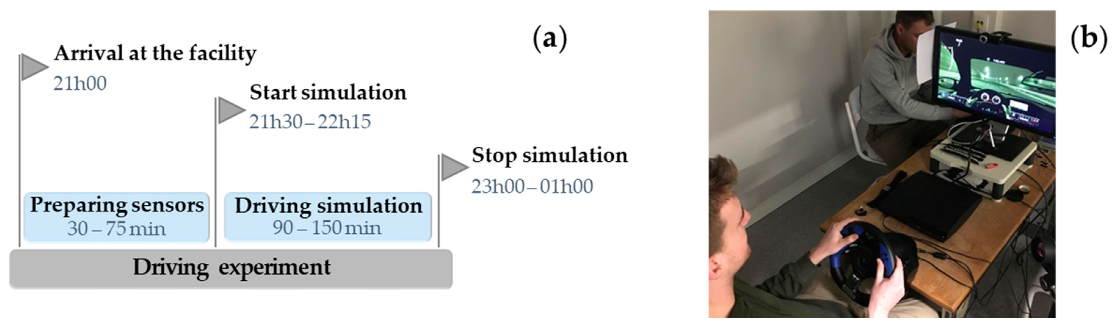
Every participant arrived at the test facility at around 21:00. After an introduction to the setup and the purpose of this study, the volunteer was equipped with the different sensors (see
Section 2.2. Data Collection). Subsequently, the driving simulation started between 21:30 and 22:15. The subjects performed the driving test in either one of the following conditions. In a first series of experiments, the lights inside the climate-controlled room were dimmed and there was no communication between the subject and the researcher present to follow up the measurements and the driver’s state. The driving simulation was stopped after a maximum duration of 2.5 h or until the driver was too sleepy to continue driving in a normal way. In a second set of experiments, the lights inside the room were left on and communication between the researcher and the participant was allowed. It has been shown that exposure to light elicits acute physiological effects in humans such as an increase in alertness, suppression of melatonin, and an increase in T
C [
24]. In line with the hypothesis by Gilbert et al. [
19], the thermoregulatory changes are thought to be related to the alerting effects instead of a direct relation between light exposure and thermoregulation. Evidently, the purpose of this second protocol was to increase the chances of staying alert during the simulation. However, the participants were not forced to stay alert. For these measurements, a maximum duration of 1.5 h was set in advance. The maximum duration was set to 1.5 h because this was the average in the first set of experiments. In other words, the first group of participants became-on average-too sleepy to drive after 1.5 h under the first conditions.
Figure 1 visualizes the timing of the experiments and shows the driving simulator that was set up in the climate-controlled room.
In total, 26 people completed the driving simulation. However, the data of 7 participants were excluded due to missing sensor data (i.e., in 3 simulation data collection were not stored correctly) and/or limited duration of the driving simulation (i.e., 5 participants were falling asleep within 40 min to 60 min after the start). In case a participant became too drowsy to drive within 1 hour, it was assumed that the process of sleep onset started before entering the simulator. As a result, the analysis was applied to a dataset of 10 participants who performed the first protocol and 9 subjects who performed the second version. Afterwards, we checked whether this first group actually experienced drowsiness during the test and the second group did not (see
Section 2.2. Data Collection).
The study was approved by the Social and Societal Ethics Committee (SMEC) of the KU Leuven (case number G-2019 04 1632) and all participants provided written informed consent before starting the driving test.
2.2. Data Collection
During the driving simulation, a number of different physiological variables were monitored. First, information about the state of the driver was obtained by means of a self-assessment of the mental state. The Stanford Sleepiness Scale (Stanford Sleepiness Scale:
https://web.stanford.edu/~dement/sss.html) (SSS) was used for this purpose [
25]. The SSS is a validated method for determining sleepiness and has been used in other studies on driver drowsiness [
26,
27]. The scale consists of 7 scores/levels to indicate the degree of sleepiness with ‘1’ being the most alert and ‘7’ being almost asleep. The driver was asked to score his/her mental state every 5 min based on this scale. The timing of these moments was indicated by the controlling researcher present in the room by a small hand gesture (i.e., slowly raising their right hand). This way, distraction from the driving task was minimal and the driver did not experience any abrupt changes in his/her mental state. When the highest score of 7 was given 2 times in a row, the experiment was terminated prematurely because we assumed the driver to be too drowsy to continue driving in a normal way. In the SSS, a score of 7 corresponds to the following state: “No longer fighting sleep, sleep onset soon; having dream-like thoughts”. Secondly, the skin temperature of the tip of the nose (T
nose) was measured using a VarioCAM infrared thermal camera with a resolution of 640 by 480 pixels (InfraTec GmbH, Dresden, Germany). The camera pas pointed towards the face and from the thermal images, the position of the nose was manually determined. The frame rate of the camera was set to 1 frame per minute. Thirdly, the skin temperature at the wrist (T
wrist) was measured continuously with an Empatica E4 wristband at a sampling rate of 4 Hz (Empatica Inc., Cambridge, MA, USA). Fourth, the heart rate (HR) was monitored using a Zephyr HxM chest strap (MedTronic, Annapolis, MD, USA). The HR, expressed in beats per minute (bpm), was sampled every second with a smartphone and app for logging the data (Samsung Galaxy J1). In this research, we did not consider raw ECG measurements because it was decided beforehand that only the HR would be used in the analyses (see
Section 2.4. Data Analysis). Lastly, the ratings of the SSS were used to check whether participants who performed the first protocol actually became drowsy during the driving test and the second group of subjects remained alert. This decision was based on the sleepiness scores. If a score of 5 was given at any point during the test, the participant was labeled as “drowsy”. If this was not the case, the subject was labeled as “non-drowsy”.
During one simulation, the data of Twrist were not stored correctly. Hence, only 18 measurements are available. In addition, the data of the heart rate were missing for 2 simulations.
2.3. Data Pre-Processing
Since there was a difference in the length of the driving simulations and sampling frequency of the different variables, the first step in pre-processing was resampling the data to a fixed number of observations for each participant. To do so, all measurements (T
nose, T
wrist, HR, and SSS) were subdivided in a fixed number of 9 windows. This specific number was chosen based on the average duration of the driving test (90 min) and the average number of SSS ratings (18 per simulation). Below,
Figure 2 visualizes this first pre-processing step schematically.
Afterwards, the mean value for the data inside each window was calculated. Subsequently, the data for each person were scaled by subtracting the average temperature or heart rate. This step was performed to account for inter-individual variability in the baseline of the variables. For instance, the heart rate of one participant fluctuated around 50 bpm, whereas this was 70 bpm for someone else. Furthermore, the slope of the data inside each window was also determined by means of least squares linear regression. These slopes will be used as the main features to distinguish between drowsy and non-drowsy drivers. A positive value corresponds to an increase in the variable in a certain window. Conversely, a negative value indicates a decrease. All operations described above were executed using MATLAB® software (The Math works Inc., Natick, MA, USA).
2.4. Data Analysis and Classification
The first step in analyzing the data was looking for significant changes of Tnose, Twrist, and HR for drowsy and non-drowsy subjects. The average trend over time was calculated for each variable as well as the distribution for each window. In addition, a Welch’s ANOVA test was performed to check whether the data of the 9 windows were significantly different in their mean. The significance level (α) was set to 5%, meaning that a p-value smaller than 0.05 indicated a significant difference. The Welch’s test was chosen because it does not assume an equal variance in both distributions.
Secondly, in our attempt to distinguish between drowsy and non-drowsy subjects, we applied a decision tree approach based on changes in skin temperature and heart rate. This methodology aims to start from biological knowledge for building our classifier, which is in contrast to traditional data-based approaches. The latter type of methods focused mainly on accuracy or performance but did not lead to physiological insights per se. In essence, this approach was inspired by the methodology described in patent EP 2 842 490 B1 published in 2016 [
28] as well as the observed trends in the data. More specifically for the skin temperatures, we expected an initial increase to facilitate heat loss for lowering the core body temperature (T
C). Afterwards, a gradual decrease in skin temperature was anticipated. On the other hand, a decrease in the heart rate was expected because energy and heat production in the body was supposed to go down. Based on this background, 3 univariate classifiers were built, which made their decisions based on the increases and decreases in the data. Hence, the classifications were performed based on T
nose, T
wrist, and HR. For the classification based on one of the temperature variables, a decision tree with 2 nodes was designed. The first nodes check whether an initial increase in the temperature occurred by evaluating the slope in the selected initial window (number 1, 2 or 3). Subsequently, the second node evaluated whether there was a decrease in temperature by looking at the slope in windows 4 to 9. Accordingly, the thresholds for both decision nodes were set to zero. Positive values for the slope corresponded to an increase in temperature and negative values to a decrease. On the other hand, for classification based on the heart rate, a decision tree with only one node assessed if HR was significantly decreasing over time.
Figure 3 shows a schematic overview of both structures for the decision tree. For the decision tree based on the temperature variables, every combination of each 2 windows was tested. For the decision tree based on HR, all windows were tested separately. Information extracted from specific windows was used for classification to indicate the position of the most valuable information present in the data. The choice for a (combination of) window(s) was based on the performance of the corresponding decision tree. For this purpose, the sensitivity, specificity, and accuracy for each combination were determined. Here a “positive” test referred to a participant being labeled as “drowsy” by the classification algorithm. The windows that were used in the decision tree with the highest accuracy were selected in the end. The receiver operating characteristic (ROC) curves and corresponding area under the curve (AUC) values were calculated as well by changing the threshold from zero. The advantage of this method is that the results allow for a meaningful interpretation since the approach is based on physiological knowledge.
In the final part of the analysis, classification was performed based on all 3 variables. For this, no predetermined structure was imposed. The only constraints were that the features (the sign of the slope inside a certain window) from the univariate classifications were used. Similarly, the sensitivity, specificity, and accuracy were used to evaluate the performance. However, it was not possible to determine ROC curves for this multivariate approach.
4. Discussion
4.1. Data Trends
From the first results presented in this study, it is clear that there are significant trends in the physiological variables of participants who became drowsy during the driving simulation. Moreover, these trends were not observed in participants that did not experience drowsiness. As expected, we observe an increase in both temperature variables in the first period of the driving simulation. This is in accordance with the fact that prior to sleep onset, the body dissipates heat via the extremities to lower the temperature of the core [
29]. During this process, blood flow to the extremities is increased (vasodilation), which in turn increases the skin temperature. The result is an increased thermal gradient with the surrounding air to facilitate heat transfer to the environment. The subsequent decrease in skin temperature is also in line with the expectations. To avoid losing too much body heat, blood flow to the skin decreases again (vasoconstriction). Besides, the heart rate of drowsy drivers decreased on average more than that of non-drowsy drivers. We hypothesize that the decreasing trend rate can be interpreted as a secondary mechanism to control T
C, which is in accordance to the statements by Kräuchi and Wirz-Justice [
20]. The human energy balance namely consists of energy producing and energy consuming (or reducing) components. Hence, the heart rate can be seen as a measure for providing energy to the body. Accordingly, lowering the heart rate means lowering the input to the energy balance. Nevertheless, we keep in mind that other physiological processes (e.g., stress) affect the heart rate and its dynamics as well. With respect to the SSS, we can infer that the test subjects evolved to a high sleepiness score in the first protocol, whereas this score did not increase significantly in the second protocol and fluctuated on average between two and three.
4.2. Decision Tree Classification
The first univariate classification based on information about the skin temperature of distal body parts (nose and wrist) shows promising results. The rather straightforward, predetermined structure of the decision trees, results in an accuracy between 68.4% and 88.9%. Moreover, AUC-values between 0.833 and 0.975 were observed. For both temperature variables, the specificity is higher than the sensitivity. This can be explained because two constraints have to be met for labeling the driver as “drowsy”, whereas he/she can be labelled as “non-drowsy” after only one decision in the decision tree (see
Figure 3). Moreover, we note that the performance for the classification based on T
wrist are better than the performance of T
nose. When analyzing the raw data of both variables, we observed smaller changes in T
wrist from sample to sample. Obviously, this was related to the much higher sampling frequency of T
wrist (see
Section 2.2. Data Collection). On the other hand, it has been shown that the temperature of the nose is also more variable. For example, it has been shown that the nose temperature changes periodically due to respiration [
30]. Alternatively, an increased sensitivity and accuracy is observed when we only consider the information of window 6 for T
nose. From this, we conclude that the decrease in temperature is a more prominent feature for distinguishing between drowsy and non-drowsy drivers. Nevertheless, only considering this feature leads to more incorrect “drowsy” classifications, which is not surprising since the physiology behind temperature changes in relation to sleep onset suggests that both an increase and decrease occur. When considering the heart rate, a negative slope in window 6 is observed for 8 out 9 drivers who reached the SSS threshold and were labelled as “drowsy”. In addition, such a decrease was also observed in half of the “non-drowsy” participants. Given the simplicity of the decision criterion, an overall accuracy of 70.6% stresses the significance of the decreasing trend in HR in our test population.
In the last section of the results, two classifications based on Tnose, Twrist and HR are presented. When the constraints for all three variables have to be met in order to label a driver as “drowsy”, only four out of eight drivers who actually experienced drowsiness were labeled correctly. In contrast, no drivers were falsely labelled as being drowsy. Accordingly, the use of such stringent constraints can be applied to situations where false positive classifications are unacceptable. In other words, this methodology can be used when it is important to be certain that a driver labelled as drowsy, is actually drowsy. Nevertheless, a sensitivity of only 50.0% is not sufficient to distinguish between drowsy and non-drowsy drivers consistently. Evidently, using less stringent constraints results in a larger number of “drowsy” labels. Hence, all 10 drowsy drivers were labeled correctly. While the specificity is now decreased, we note that still 7 out of 9 non-drowsy drivers are correctly identified. This last classification resulted in an accuracy of 89.5%.
When comparing the different classification approaches, we note that the univariate classification for Twrist and the second multivariate classification resulted in similar accuracies (88.9% and 89.5%). Moreover, both results cannot be compared directly because the number of samples differs. The fact that a single temperature variable performs equally well as the multivariate classification indicates that including the heart rate for classifying the data does not add significant value to the current analysis.
4.3. Comparison to State-of-the-Art Methods for Drowsiness Detection
When comparing the performance of these classifications to related work on detecting driver drowsiness, we first note that, to our knowledge, no other studies make use of distal skin temperatures in their classification. Furthermore, only the patent by Berckmans et al. [
28] presents a method based on similar signals, namely distal ear temperature and heart rate. Here, different conceptual approaches are described as well as the performance of one such method for a training and validation set; respective accuracies of 87.5% and 72.7% were obtained. On the other hand, multiple studies present methodologies to detect or monitor drowsiness based on information about the heart rate. More specifically, features related to heart rate variability (HRV) are most often used. For instance, Li and Chung [
31] present a detection algorithm with an accuracy, sensitivity, and specificity of 95% each. In this study, two-minute-long drowsy and alert events were classified based on the ratio of low (0.04–0.15 Hz) to high frequency (0.15–0.40 Hz) variability in the heart rate obtained from photoplethysmography. In another study, ECG measurements were used to detect drowsiness based on HRV as well as respiratory frequency [
32]. Here, a positive predictive value (PPV), sensitivity, and specificity of 96%, 59%, and 98%, respectively, was reported. In addition, an accuracy of around 78% corresponds to these results. In contrast to the two prior studies which used behavioral signs as a reference for the state of the driver, Fujiwara et al. validated their HRV-based drowsiness detection with EEG measurements [
33]. Here, the algorithm was successful if drowsiness was indicated in a period of 15 min before sleep onset (NREM sleep stage 1). In 12 out of 13 subjects, sleep onset was detected in this timeframe. In comparison to these studies, our classification based on only the heart rate performs less well (an accuracy of 70.6%). However, HRV is interpreted as a measure for the dynamic control of the heart by different parts of the nervous system. In this study, the heart rate was interpreted as a part of the heat balance inside the human body. More specifically, HR represents the rate of aerobic heat production inside the body. Therefore, we also consider HR in combination with other components of the heat balance. Nonetheless, using ECG measurements in future research could make it possible to combine or compare these different approaches.
To put our own results further into perspective to the state-of-the-art, a couple of recent studies that used completely different variables and features are discussed hereafter. Firstly, Li et al. [
34] present a smartwatch-based wearable EEG system for driver drowsiness detection. They designed a headband with three dry electrodes, instead of 21 electrodes used in the standard 10–20 system. In their analysis, they distinguished between “alert” and “drowsy” epochs that were labelled based on the percentage of eye closure (PERCLOS) and the number of adjustments on the steering wheel. The authors reported an average accuracy of 91.25% and 91.92% for detecting the alert and drowsy epochs, respectively. Secondly, Mandal et al. [
12] developed a method to determine PERCLOS from images of a dome camera in a bus. Their results showed a matching rate between their method and a ground truth measure for PERCLOS of 85.02% and 95.18% for normal and fatigued drivers, respectively. Since their method was based on commercial technology that is already implemented in busses, monitoring bus drivers can be done unobtrusively. Thirdly, the work by Li et al. [
13] presents yet a completely different approach. The fatigue level, scored by experts, was linked with data about the steering wheel angles (SWA) recorded under real driving conditions. The system was able to run on-line and performed with an accuracy of 78.01% in distinguishing drowsy from non-drowsy participants. In this research, we obtained accuracies between 70% and 90%, which is below the performances of the related state-of-the-art. Nevertheless, the results show potential for future research.
Lastly, it should be noted that each study applies different protocols and builds their classifier on different events or epochs. This makes it even more difficult to compare all results directly.
4.4. Current Limitations and Future Perspectives
Given the preliminary nature of this pilot study, several limitations and suggestions for future work are listed in this section. Firstly, more advanced methodologies and equipment will improve the quality of the obtained measurements. For instance, now a simple driving simulator is used as a basis for the experiments. Nowadays, there are simulators available with a driving experience very close to driving a real car. Nevertheless, when working with a simulator, lacking the danger of causing an accident is thought to affect the driver in his behavior [
35]. On the other hand, purposely sending out drowsy drivers on the road would be unethical and illegal. Using wearable technology for ambulatory monitoring of the driver in real-life conditions might be a good alternative for this issue. Furthermore, applying a crossover study design in which each participant performs the driving test in drowsy and non-drowsy conditions would allow for a pairwise comparison of the individual direction and magnitude of the changes in thermoregulation. This is not possible with the current data since each driver only performed the test one time. Another way to improve the experimental work is by working with more advanced measures for determining the state of the driver. Now, each driver evaluates his/her state of alertness based on the SSS. Presumably, individual differences in the interpretation of each level of the SSS causes variability in the data. The use of EEG measurements (brain activity) could provide a solution to this issue. As mentioned, EEG is used as a gold standard in sleep research. Alternatively, scoring the driver’s state based on an expert’s opinion is also done in the literature. An expert can be trained in scoring the driver based on behavioral expressions. Although such a score is also the result of human interpretation, the variability due to a difference in the scorer is eliminated. A final remark on the applied methodology is the timing of the simulations. Currently, one fixed moment throughout the day is selected to perform the driving simulation. By executing the measurements at different moments, a generalization of the results is possible. For instance, Fujiwara et al. [
33] used data collected at 11:00 and after lunch. However, we have to keep in mind that the theory behind this method is related to actual sleep onset and does not relate directly to short drops in attention throughout the day. Accordingly, future research on the proposed methodology will focus on this specific type of event. Related to the timing of these events, we expect that the observed physiological changes do not only occur at night. For instance, night shift workers have an altered sleep-wake cycle. In general, diurnal changes in body temperature and heart rate follow the daily activity-rest cycle [
36].
Secondly, we discuss a number of limitations related to data analysis. At the moment, we applied a very straightforward method to determine significant differences in drowsy and non-drowsy drivers. Subdividing the measurements in a fixed amount of time windows was an inevitable part of the analysis. As mentioned, this is due to a difference in the length of the experiments. By applying the windows to the data and extracting the average value and the slope, a lot of detail, as well as information about the timing is lost. Nevertheless, this did not prevent us from identifying significant trends in the data and successfully distinguishing between drowsy and non-drowsy drivers. A follow-up study could either perform experiments of the same length or apply a time series approach to detect drowsiness over time and pinpoint key moments in the transition from an alert state to a drowsy one. Additionally, to allow for such a methodology to be applied in real-time and real-world situations, future research has to focus on using techniques such as recursive estimation and online time-series analysis to determine the increases and decreases in the variables in real-time. Overall, the current methodology for distinguishing between drowsy and non-drowsy drivers is elegant in its simplicity, allowing for a physiological interpretation of the results and indicates the potential of using thermoregulatory features for drowsiness detection. A final remark on the analysis is related to the lack of data for validation. Due to the limited number of measurements, no proper validation technique could be applied to the current dataset. Leave-one-out cross validation was briefly considered, however, this resulted in the same results for the training and test set. More specifically, only the selected window number could vary when using the decision tree classification. The selection for a (combination of) certain window(s), did not vary when only leaving out one observation at a time. Naturally, the lack of validation is identified as one of the most important limitations of the current communication.
5. Conclusions
In this work, the use of features extracted from distal skin temperatures and heart rate is tested for detecting drowsiness in driving simulations. In the first part of the analysis, we demonstrated that Tnose, Twrist, and HR vary throughout the measurement in a specific pattern in participants who became drowsy. Initially, the temperature measured at the nose and the wrist increased to a maximal value. Subsequently, a gradual decrease in these temperature variables was observed. When studying the heart rate of the driver throughout each simulation, a significant decrease was observed in both drowsy and non-drowsy participants. However, the decreasing trend was more distinct in the group of drowsy drivers. Secondly, we showed that both populations of drivers (drowsy and non-drowsy) could be classified based on these observed trends in the data of Tnose, Twrist, and HR. Despite the simplicity of these classifications, their performance indicates the potential for future research. The main advantage of the applied methodology is that it is based on knowledge about physiological processes related to sleep onset. Specifically, heat loss via the extremities and controlling of the heart rate regulates the decrease in core body temperature before and during sleep. A secondary classification approach was tested by using the information of all three different variables at the same time. From this analysis, we conclude that including the heart rate in our classification approach does not improve the performance significantly. Lastly, the current results were compared to the state-of-the-art in drowsiness monitoring and several limitations and suggestions for future research have been discussed.


