Article

GA Optimization Method for a Multi-Vector Energy System Incorporating Wind, Hydrogen, and Fuel Cells for Rural Village Applications

1
Electrical Engineering School, Guizhou University, Guiyang 550025, China
2
School of Engineering & Applied Science, Aston University, Birmingham B4 7ET, UK
3
Department of Engineering Science, University of Oxford, Oxford OX1 3PJ, UK
*
Authors to whom correspondence should be addressed.
Appl. Sci. 2019, 9(17), 3554; https://doi.org/10.3390/app9173554
Submission received: 20 July 2019 / Revised: 20 August 2019 / Accepted: 21 August 2019 / Published: 30 August 2019
(This article belongs to the Special Issue Advancing Grid-Connected Renewable Generation Systems 2019)

Abstract

:
Utilization of renewable energy (e.g., wind, solar, bio-energy) is high on international and governmental agendas. In order to address energy poverty and increase energy efficiency for rural villages, a hybrid distribution generation (DG) system including wind, hydrogen and fuel cells is proposed to supplement to the main grid. Wind energy is first converted into electrical energy while part of the generated electricity is used for water electrolysis to generate hydrogen for energy storage. Hydrogen is used by fuel cells to convert back to electricity when electrical energy demand peaks. An analytical model has been developed to coordinate the operation of the system involving energy conversion between mechanical, electrical and chemical forms. The proposed system is primarily designed to meet the electrical demand of a rural village in the UK where the energy storage system can balance out the discrepancy between intermittent renewable energy supplies and fluctuating energy demands so as to improve the system efficiency. Genetic Algorithm (GA) is used as an optimization strategy to determine the operational scheme for the multi-vector energy system. In the work, four case studies are carried out based on real-world measurement data. The novelty of this study lies in the GA-based optimization and operational methods for maximized wind energy utilization. This provides an alternative to battery energy storage and can be widely applied to wind-rich rural areas.

1. Introduction

The technologies of integrating renewable energy into smart grids are booming where renewables, including wind, solar and bio-energy, have become promising resources around the globe [1,2]. Taking the UK for example, renewables from wind, solar, hydro, and biofuel take up 26.6% of the total electricity generation [3]. Remarkably, wind energy is a major contributor to renewable power generation, which accounts for 45% of the total renewables. For villages with grid connections, electrical power generated from renewables can be fed into the main grid. For off-grid villages, the generated electricity needs to be stored (e.g., in batteries) to balance load and demand. Presently, wind–hydrogen–fuel cell-based power systems are researched only in laboratories while their industrial applications are hampered by low system efficiency and high costs [4]. In order to address these issues, an effective and optimized operational scheme is needed to schedule the operational events and to manage power flow between the different components. Therefore, energy storage is necessary to store a certain amount of electricity during the off-peak hours and then output it during peak hours [5,6,7,8,9,10].

2. State-of-the-Art Technologies

In the literature, a hybrid system incorporating photovoltaics (PV), fuel cells (FC), and ultra-capacitors (UC) is reported for stand-alone applications. In this system, the FC provides additional power when PV cannot meet load demand. If the demand further exceeds the FC capability, the UC bank starts and joins the supply. Reference [11] reports an experimental study based on a hybrid system including PV panels, wind turbines, biomass gasification plants, and a battery bank for energy storage. The feasibility of the hybrid system was verified, and the control strategy was set up according to battery charging status. If the state of charge (SOC) goes down to 50% of its nominal value, the biomass gasification plant starts to work to provide power. In reference [12], a hybrid syngas/solar PV/battery power system was developed for off-grid applications. During the running tests, the solar PV/battery system with a standby syngas genset ran reliably to meet the changing power demand. Similar to [11], the batteries aid in the power supply if the demand exceeds the intermittent solar power. The operational strategy of the genset was based on the batteries’ SOC. The genset automatically started to operate and supply power to both of the load and the batteries when their SOC dropped to 40% and stopped charging the batteries when their SOC reached 80%. Reference [13] developed a hybrid PV–engine system and an optimization strategy for SOC control combined with minimum costs. Another study presented in [14] showed a hybrid system combining PV, wind, and bio-gas genset to power a sewage plant. In general, these systems are effective in providing required power to meet the demand but suffer from the lack of systemic optimization in coordinating the different power generators to achieve the best system performance (e.g., utilization of renewables, energy efficiency, and operating cost).
Moreover, the genset as a backup supply is bulky and expensive. In this regard, fuel cells based on proton exchange membrane (PEM) provide much promise. These are more efficient and environment friendly. They can conveniently convert the chemical energy stored in hydrogen and oxygen into electricity [15,16,17,18,19] and be interfaced with an AC or DC distribution system using different power electronic converters [20]. In reference [21], the authors studied energy efficiency when the FC supplied electricity to the load and/or the AC grid in residential environments. Their operational strategy was based on the phase angle and voltage variation of the output so as to control a FC-based power system [22]. Steady state behavior and the dynamic voltage variation of the FC were predicted based on empirical and test results. In [23], an energy management optimization strategy for a hybrid wind–batteries–FC system was designed to realize cost-effective operation of the hybrid system. It was found that the FC system can meet the excessive power demand for a reasonable time if the wind power cannot satisfy the load demand whilst the ultra-capacitor can only supply power for a shorter duration. In this work, the system can tolerate the rapid changes in wind speeds and suppress the effects of these fluctuations. The optimization and integration of hybrid renewable energy hydrogen fuel cell energy systems are critically reviewed in reference [24]. The effect of the fluctuation range of the power output on the hydrogen production devices, in terms of equipment lifespan and hydrogen purity, in a wind–hydrogen system cannot be omitted [25]. The data analysis in reference [26] indicated that the hydrogen content was stabilized between 1.04% to 1.10% in the load range of 20% to 100% in the water electrolysis system, which meets the safety standards. The current status and development trend of wind power generation-based hydrogen production technology have been recently reviewed in reference [27]. Overall, the existing systems are capable of operating with stable distributed systems and large loads for long durations (in hours) [4,28,29,30]. However, these studies have not fully optimized power distribution in the multi-vector energy (mechanical, electrical, and chemical forms). Furthermore, it is more challenging to operate a micro distributed power system for village loads where the load can change from hundreds of watts to over tens of kilowatts rapidly.
This paper is focused on a wind–hydrogen–FC powered multi-vector energy system for household applications. The novelty of this study lies in a new operational method which was developed to maximize the local usage of wind energy. The power flow among different components were analyzed and optimized for the whole system, based on a genetic algorithm (GA) optimization method. System state variables, operational variables, and the objective functions were defined under the state space model (SSM). A GA was developed to solve the optimization problem so as to control power flow between different components in the system. By doing so, the majority of wind power is used to supply the load and generate hydrogen/oxygen while there is only limited wind energy over a certain period which is fed into the grid.
The rest of the paper is arranged as follows: Section 2 presents the system configuration, the energy flow within the system, and the analytical models with a set of equivalent functions. Section 3 provides the methodology for operational strategies in this investigation. Section 4 discusses and analyzes the test results using real-world data. Section 5 summarizes the key findings and suggests some future work.

3. Principles of Operation

The proposed system is shown in Figure 1. It consists of a wind turbine generator, a water electrolyzer, a fuel cell module, a DC/DC converter, and two DC/AC power converters and an AC/DC converter. In this system, wind energy is firstly converted into electricity, fed to the grid and used to electrolyze water to generate hydrogen and oxygen. Hydrogen and oxygen are stored in two separate storage tanks. The DC bus is a single phase rated at 230 V. The electrolyzer takes electricity from the DC bus to generate hydrogen and oxygen, which is later used for the FC module to reproduce electricity.

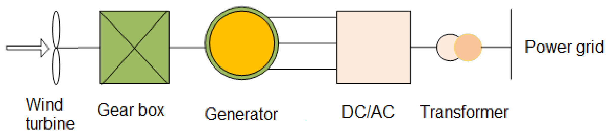
3.1. Wind Energy Conversion

Conventionally, a wind energy subsystem is illustrated in Figure 2. The physical subsystem consists of a wind turbine, a gear box, a generator, a DC/AC converter, and a transformer linking to the power grid. In this study, energy loss over the power conversion processes is ignored. Wind power can be expressed by Equations (1) and (2).
Equation (1) presents the relationship between the wind speed and the mechanical power.
p w t = { 0 ,     i f   v < v c u t _ i n   o r   v > v c u t _ o u t                 v v c u t _ i n v r v c u t _ i n · P r   ,       i f   v c u t _ i n v   v r     P r   ,       i f   v r < v v c u t o u t
where p w t , P r , v c u t _ i n , v c u t _ o u t , v r and v represent the output power, nominal power, input wind speed, output wind speed, nominal wind speed, wind speed at the turbine blade tip.
p w i n d = 1 2 · ρ · A · v 3
Equation (2) is another calculation method of electrical power output. p w i n d , ρ , A and v stand for the wind power, air density, equivalent area, and average wind speed, respectively.

3.2. Hydrogen and Oxygen Production

Equation (3) represents the percent   f w f of the wind power being used for water electrolysis where the power consumed is p e .
p e = p w i n d · f w f
In general, the volume ratio between hydrogen and oxygen by the water electrolytic process is around 2:1. Thus the flow rate of the production can be calculated by:
V H 2 = 2 · V O 2 = 418 · p e · η w e / U n
where V H 2 , V O 2 , η w e , U n refer to the hydrogen flow rate (liter/hour), oxygen flow rate (liter/hour), transformation efficiency, and the voltage of the electrolytic bath, respectively.
Hydrogen and oxygen production should be within the minimum and maximum capacity of the FC equipment. Moreover, the storage levels are limited by the device capacity. The constraints are expressed as
V H 2 m i n V H 2 V H 2 m a x
0 < η w e < 1
ω O 2 Ω O m a x
ω H 2 Ω H m a x
where V H 2 m i n , V H 2 m a x , ω O 2 , ω H 2 , Ω O m a x , and Ω H m a x refer to the minimum and maximum capacity of the hydrogen production, oxygen storage volume, hydrogen storage volume, maximum capacity of the oxygen storage, and the maximum capacity of the hydrogen storage, respectively.

3.3. Fuel Cells

The actual output voltage of the PEM fuel cell, E c e l l , is lower than its equilibrium potential due to irreversible losses. The losses include the polarization or overpotential originating primarily from activation loss, ohmic loss and concentration loss. E c e l l is a function of the output current density, temperature, partial pressure of reactant.
E c e l l = E 0 η a c t η o h m i c η c o n
where E 0 is the open-circuit potential or thermodynamic equilibrium potential, η a c t , η o h m i c and η c o n are over-potentials with respect to activation, ohmic and concentration losses, respectively.
The power density during the PEM fuel cell operation is given by
P = i · E c e l l
where i is the current density.

3.3.1. Open-Circuit Potential

The open circuit potential (OCP) is the theoretical or equilibrium potential of an electrode in the absence of an external current flowing to or from the electrode, which can be calculated based on the knowledge of thermodynamics. The portion of the reaction enthalpy that can be converted into electricity in a fuel cell corresponds to the Gibbs free energy.
Δ G = Δ H T · Δ S
In this equation, the Gibbs free energy Δ G is not equal to the total reaction enthalpy Δ H because there are some irreversible losses in energy conversion due to creation of entropy Δ S .
In general, the electrical work is a product of charge and potential:
W e l = q · E
where W e l is the electrical work, q is the charge and E is the potential.
The total electrical charge transferred in a fuel cell reaction per mole of H2 consumed is
q = n · N · q e l
where n is the number of electrons per molecule of hydrogen ( n = 2 ), N is the Avogadro’s number ( N = 6.022 × 10 23 molecules per mol), q e l is the charge per electron ( q e l = 1.602 × 10 19 C per electron). Because q e l N = 9.65 × 10 4 C mol−1 is the Faraday’s constant F , the electrical work is therefore:
W e l = n · F · E
Therefore:
W e l =   Δ G
The theoretical potential of a fuel cell is then given by
E = Δ G n · F
The temperature-dependent theoretical cell potential can be calculated by substituting Equation (11) into Equation (16).
E = Δ H T · Δ S n · F
The theoretical cell potential also varies with reactant pressure. Assuming the reactants and product behave as an ideal gas, the change in the Gibbs free energy in an isothermal condition is expressed by
d G = R · T · d p p
Carrying out an integration process:
G = G 0 + R · T · ln ( p p 0 )
where G 0 is the Gibbs free energy at the standard condition (25 °C and 1.0 atm), and p 0 (1.0 atm) is the reference or standard pressure.
This is known as the Nernst equation. Assuming the water is produced in the gas phase. The OCP can be calculated as
E 0 = ( Δ H T · Δ S ) n · F + R · T · ln ( p H 2 · p O 2 0.5 p H 2 O )
As shown in Figure 3, the OCP decreases with the temperature in a linear manner. In addition, the OCP for liquid water production is higher than that for water vapour.

3.3.2. Activation Loss

The major polarization is the activation loss, which is pronounced in the low and medium current density regions. In these regions, electronic barriers must be overcome before the advent of current and ionic flow. The activation loss is directly proportional to the current density, which can be expressed as follows:
η a c t = R · T α · n · F · ln ( i i 0 )
where R is the universal gas constant, T is the temperature, α is the charge transfer coefficient, n is the number of electrons involved, F is the Faraday constant, i is the current density and i 0 is the exchange current density. The activation loss is due to the sluggish electrochemical reactions at the electrode surface, at which the fuel is oxidized and the oxidant is reduced. The activation barrier must be overcome by the reaction species in successful fuel cell reactions.

3.3.3. Ohmic Loss

The power loss as a result of resistance to the electrons and ions flowing through the electrode is known as the ohmic loss. It varies over the entire range of the current density due to the nature of fuel cell resistance. The ohmic loss is represented by
η o h m = i · ( R e l e +   R i o n )
where R e l e and R i o n are the electronic and ionic resistances, respectively. It has been reported that the ionic resistance is predominant in most FC cases due to the very high electronic conductivity of the graphic-based current collector. The ionic resistance of the proton exchange membrane depends on its water content, which is in turn a function of the temperature and current density. The ionic resistance is given by
R i o n = I M · r M A
where l M is the membrane thickness, A is the active cell area, and r M is the membrane resistivity, expressed by
r M = 181.6 · [ 1 + 0.03 · ( i A ) + 0.062 · ( T 303 ) 2 · ( i A ) 2.5 ] [ λ 0.634 3 · ( i A ) ] · exp [ 4.18 · ( T 303 ) T ]
where λ is the water content of the membrane and T is the temperature.

3.3.4. Concentration Loss

The concentration of the bulk fluid drops as the reactant gases are consumed at the electrode through the electrochemical reaction. This leads to a concentration gradient within the electrode. The concentration loss occurs over the entire range of current density, and becomes prominent at high current density. Under this condition, the electrochemical reaction is much faster than that of species transport, making the gas reactant difficult to reach the reaction sites inside the porous electrode. The concentration loss can be represented by
η c o n = R · T n · F ln ( 1 i i L )
where i L is the limiting current density.
Figure 4 illustrates the cell potential as a function of the current density, with respect to activation loss, ohmic loss, and concentration loss.

3.3.5. Fuel Cell Efficiency

The efficiency of a fuel cell operated at different loads can be expressed in terms of the ratio of the actual output voltage to the ideal cell voltage. The actual output voltage is lower than the ideal cell voltage owning to the voltage drop.
c e l l   e f f i c i e n c y = E c e l l E 0 · 100 %
where the actual output voltage E c e l l at different current density levels can be obtained from Equation (26).

3.4. Energy Flow in the System

In order to optimise the power flow in the system, an energy flow chart is used to demonstrate the contribution of each component to the system. Based on the connection and conversion between them, the variables for the optimization process are derived and explained in the following section.

3.4.1. Equivalent State of the Charge of the Energy Storage System

A water electrolyzer, the hydrogen/oxygen tanks, and the fuel cells constitute the energy storage system in this study. Hydrogen and oxygen are generated by consuming electricity in the similar way as charging batteries. Then the fuel cell regenerates electricity by consuming hydrogen and oxygen while the amounts of hydrogen and oxygen decrease gradually. In order to evaluate the remaining hydrogen and oxygen levels in the storage tanks, an equivalent state of charge is introduced as shown in Equations (27)–(29).
E S O C H = P h P h 0
E S O C O = P o P o 0
E S O C S = E S O C H · V H + E S O C O · V O V H + V O
where E S O C H and E S O C O are the levels of the hydrogen and oxygen tanks, respectively; P h , P h 0 , P o and P o 0 are the current pressure of the hydrogen tank, the full pressure of the hydrogen tank, the current pressure of the oxygen tank and the full pressure of the oxygen tank, respectively. E S O C S , V H , and V O represent the equivalent state of the charge of the storage system, the volumes of the hydrogen tank and the oxygen tank, respectively. For the safe operation of the storage systems, the level of the E S O C S is controlled between 0.2 and 0.9.

3.4.2. Energy Flow Chart

An energy flow chart is shown in Figure 5. Wind energy is the only energy source for the whole system. Wind power is mainly used to supply electrical demand of the targeted household application. This portion of wind power denotes p d i r ( k ) . The rest of wind power is stored in the form of hydrogen and oxygen via water electrolysis while the power consumed is p H 2 O ( k ) . The extra energy generated by the wind turbine is fed to the smart grid. In case the demand exceeds the wind power, the fuel cell starts to generate electricity and act as the back-up power supply.

4. SSM-GA Optimization for Energy Management

In essence, GA is inspired by natural selection and genetic mechanisms in biological evolution. It is a stochastic optimization method that was introduced and developed by Professor Holland in 1975. It uses crossover and mutation to manipulate a genetic operator to search and find the best solution candidates while its fitness function reaches its optimal value (maximum or minimum) over the horizon. In this study, GA is used to find a set of E S O C S ( k ) allowing the maximum wind power be consumed locally over the optimization process. In order to derive the relationship between each energy component (an SSM expression), a conventional method to describe the complex multi-vector energy system is used. In addition to the constraints in the operation, the SSM is also the main constituent of the GA fitness function to derive the relationship between the variables.
A flow chart for the GA optimization is illustrated in Figure 6.
In the process, the best soluation is found untill the stopping criterion is met. There are 6 steps as follows:
  • An initial solution is randomly selected between 0.2 and 0.9. For instance, the state variable in the SSM could be { x ( i ) i = 1 24 | [ 0.213 , 0.334 , 0.257 0.720 ] } ;
  • A new generation of solution candidate is applied to the fitness function. The fitness function in this study consists of the SSM function and a series of constraints. An SSM function represents the correlation between the variables x ( i ) , x ( i 1 ) and y ( i ) while the constraints are defined;
  • If the solution candidate satisfies the stopping criterion and the objective function is met;
  • Crossover and mutation methods are used to generate a new solution candidate;
  • Under the operation of the GA function, a new generation is created;
  • A final solution is found when the GA optimization ends.
In this study, the GA optimization and the associated fitness function are programmed by MATLAB.

4.1. SSM and Fitness Function

In an SSM, each state which includes one or more components (state variables) is a timing sequence. The current state is coherent to the previous state. In essence, the target of GA is to find the best decision set over the optimal horizon while its optimal objective is included in its fitness function.
In the system, energy balance equation can be expressed as Equation (30).
p d i r ( k ) + p f c ( k ) = p l o a d ( k )
where p g r i d ( t ) , p l o a d , p f c refer to the power from the wind turbine, load, and fuel cell, respectively.
In order to structure a state-space representation, two state variables and one output variable are defined as follows.
x 1 ( k ) = E S O C S ( k )
x 2 ( k ) = y ( k ) = p d i r ( k )
The state space model can be presented as
x 1 ( k ) = x 1 ( k 1 ) + ξ 1 · x 2 ( k ) + ϕ 1
y ( k ) = x 2 ( k )
Besides, there is an energy balance equation for calculating the wind power fed into the grid.
p d i r ( k ) + p H 2 O ( k ) + p g r i d ( k ) = p w i n d ( k )
or
p g r i d ( k ) = p w i n d ( k ) p d i r ( k ) p H 2 O ( k )

4.2. GA Optimization Process

In the optimization, there are two constraints to define the searching boundary.
0.2 E S O C S ( k ) 0.9
0 p g r i d ( k ) p w i n d ( k )
The aim of the optimization is to minimize the power sending to the grid while most of the wind power is consumed locally. Therefore, the objective function can be defined by
f ( x ) = m i n k = 0 24 p g r i d ( k )
s. t.
p d i r ( k ) + p H 2 O ( k ) + p g r i d ( k ) = p w i n d ( k )
p d i r ( k ) + p f c ( k ) = p l o a d ( k )
0.2 E S O C S ( k ) 0.9
0 p g r i d ( k ) p w i n d ( k )

5. Results and Analysis

This section analyzes the features of energy demand in the targeted application and wind energy characteristics.

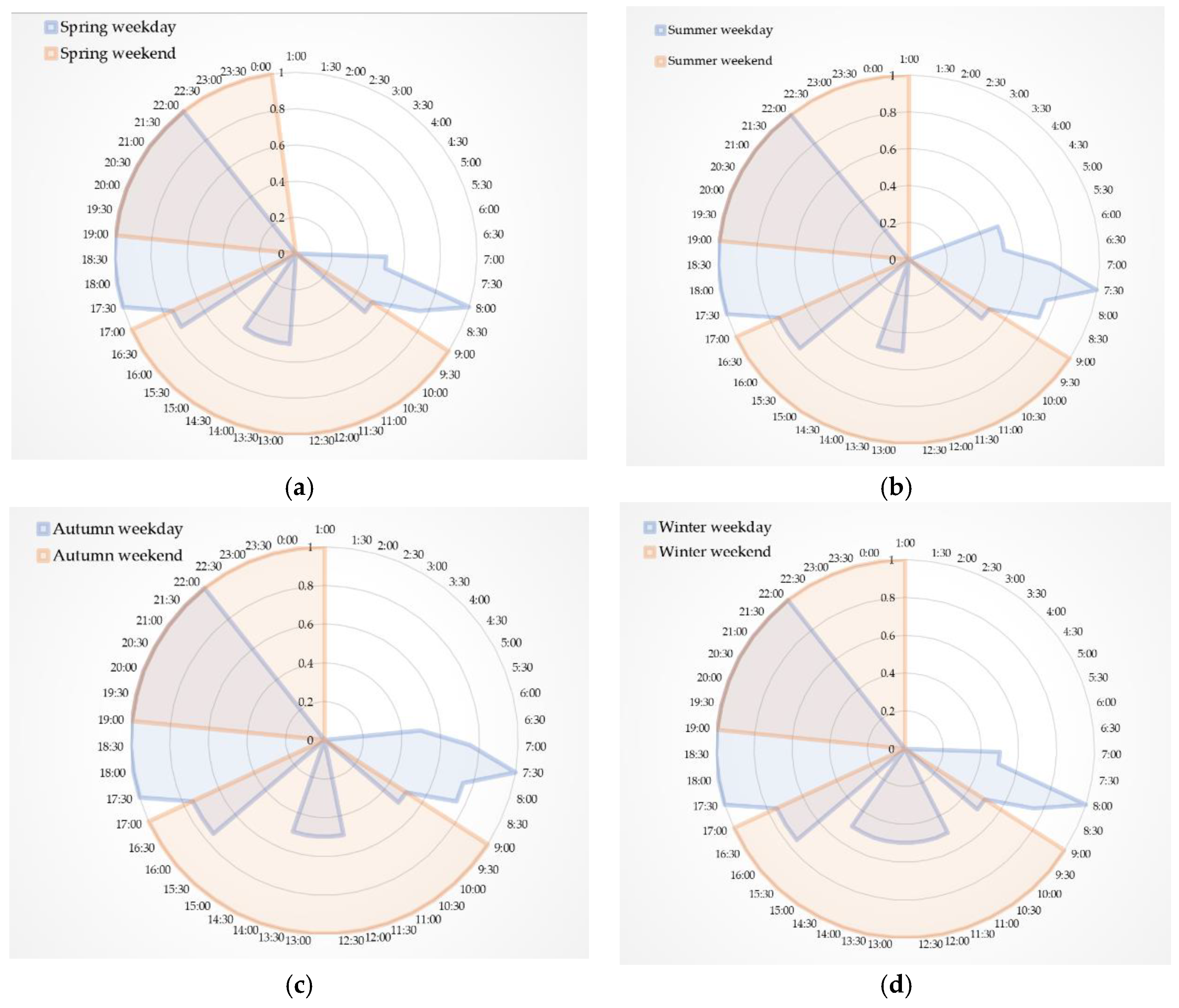
5.1. Consumption Characteristics of the Household Application

The investigated household was a two-bedroom domestic house which is a typical UK family home [31]. The activity schedules were recorded over one year as illustrated in Figure 7. Each diagram demonstrates both weekday and weekend scenarios in each season as Figure 7a–d shown.
Similar activity patterns are discovered according to the four diagrams. These weekday activities can be generally divided into three patterns, including a morning section, a mid-day section and an evening section. On a spring weekday, the three sections start from 7:00, 13:00 and 16:30 respectively as shown in Figure 7a. From 7:00, the occupants carry on different activities. The morning section starts at 5:30 on a summer weekday (Figure 7b) which is earlier than other seasons. The irregular polygon in morning section shows that the occupant number varies obviously in morning section because that family members have different daily schedules on the weekdays. The autumn day (Figure 7c) has a quite similar pattern to the spring day except that each section in autumn starts earlier than that of the spring day. For example, the morning section in autumn starts from 6.30 which is half hour earlier than spring. The midday section in winter (Figure 7d) starts slightly earlier than that in other seasons since occupants might come back home earlier in winter due to cold weather. Winter weekdays have the most occupancy hours (11:00 to 15:00). The weekends can be divided two sections, day and night sections. Weekend activities in four seasons are almost the same except that the spring night section ends earlier than other seasons. These discrepancies give rise to the variations of energy consumption.

5.2. Demand Profiles in Case Studies

In this work, four different daily electricity consumption patterns in four seasons were investigated to validate the proposed methods. The key features of power generation and demand in a village user are summarised in Table 1 while the waveforms in Figure 8 display the demand profiles in these days.
As given in Table 1, the load changes from 0 to 5.8 kW on the spring day. The power demand raises to 9.7 kW on the autumn day. The autumn day consumes the highest energy (16.1 kWh) over the next three days. The winter day also consumes significant energy as poor illuminance and cold weather increase lighting and heating requirements. In terms of the period and the percentage of the low demand, four season days display a similar trend while winter and autumn consume more power than spring and summer in general. In Figure 8, a similar trend is shown that the peak hours on four typical days were less than 1 h even on autumn and winter days. The three ranges, named the morning section, the midday section and the evening section, are found in Figure 8. Taking the spring day for example, the consumption increased from 6:30 in the morning and reached the peak at 8:15. Afterwards, the consumption fluctuated before decreasing to below 1 kW. From 13:00, the consumption increased again till 14:00. In this midday section, the energy consumption also fluctuated because different appliances were used over this period. 17:00 saw a consumption peak and the next peak occured around 19:00. The three sections were less distinctive on the selected winter day since this day was a weekend and the occupants had a different activity schedule to the weekday.

5.3. Wind Speed and Power Profiles

The average wind speed was measured and recorded on the test site, which ranged from 0 to 21 m/s to produce the power from 0 to 4 kW, as shown in Figure 9. Each season has strong wind speed, however, there is no fixed pattern available in any given season. The four diagrams in Figure 10 illustrate the wind power variations for each single day. The spring day in Figure 10a showed that the wind power gradually decreased from the peak of 1.4 kW at 1:00 to the lowest point at 11:00. It maintained this low value to 16:00. Afterwards, the wind power slowly increased to 0.5 kW around 21:00. The summer day in Figure 10b had a power output below 1 kW over most of the day except the peak power at 20:00. The wind power had relatively low variations in the autumn day with the maximum value 1.2 kW at 12:00, as seen from Figure 10c. The wind power in the winter day ranged from 0.2 to 0.9 kW with some variations, as shown in Figure 10d. The waveforms show the wind power. By comparison, more energy was generated in the autumn and the winter days than that in the spring and summer days. The summer day provided the least energy to the system among those chosen days.

5.4. Analysis and Discussion

In this study, both the domestic demand and wind energy were intermittent but their variations presented completely different features. The hydrogen-based energy storage system is therefore needed to bridge the gap between the two while a GA algorithm is used to maintain the optimal operation of the energy storage system.
These features can be summarized as follows:
  • The peak demand is over 4 kW but it only lasts for a couple of minutes. The demand is 4 kW in summer days and below 1 kW on winter days;
  • The energy demand has 3 peaks over selected days while the wind power is random on these days.
  • The peak demand and the peak supply do not occur in the same time on any selected days.
  • In general, the wind power is higher than the energy demand over the night time on any chosen days.

5.4.1. E S O C S Variations

Figure 11 demonstrates the test results of E S O C S for the selected four days. In the case of the spring day, E S O C S increased from 0:00 to 7:30. Over the period, the energy demand is low while the wind power maintains a relatively high output. Most of wind energy is used to charge the storage system (hydrogen generation via electrolysis). Afterwards, the wind power and E S O C S decrease while the energy demand is met by both the wind power and the fuel cell, as shown in Figure 11a.
In Figure 11b, E S O C S presents a continuous growth from 0:00 to 5:00 until reaching its upper limit (0.9). From 6:30 onwards, it dramatically decreases until 14:00. E S O C S reached its upper limit at 20:00 again after some fluctuations. In the summer day, a fast and continuous growth is seen as the wind is strong while a decrease is seen due to the demand over the wind energy supply.
The autumn day in Figure 11c also presented some fluctuations. E S O C S kept growing over the night until 6:30 when the energy demand was higher than the wind energy. From 9:30 onward, E S O C S recovered and grew to its upper limit from 12:00 to 17:00 before meeting a peak demand in the afternoon. Afterwards, E S O C S declined until reaching its low limit (0.2).
E S O C S on the winter day maintained higher than 0.5, as shown in Figure 11d. The main decline occured at 9:00 and 17:00 when both morning and evening peak demands start. After peak demands, E S O C S started to rise as more power from wind turbines was used to charge the storage system.

5.4.2. Fed-in Power to the Grid

Four diagrams in Figure 12 illustrates the power fed into the grid. It can be seen from Figure 12a that the spring day hardly provided any wind energy to the grid while the wind power was totally used to supply the domestic demand or charge the energy storage system. The winter day fed the most wind energy to the grid, as shown in Figure 12d. This is because that the wind power generated was more than the local need on that day. There are two periods on the summer day that the wind power was fed into the grid, as given in Figure 12b. One period is from 4:00 to 6:00 prior to the morning peak demand. Another one started at the peak wind power at 20:00. Most of the fed-in wind power occurred between 12:30 and 16:30 where E S O C S was fully charged. As can be seen in Figure 12c, the extra power from the wind turbine was fed into the grid between 12:00 to 17:00 while E S O C S kept the upper limit with no need for charging or discharging the storage system.

5.5. Key Performance Indicators

Power, energy and equivalent level of storage are discussed in this section. Table 2 summarizes the main indicators of the system components.

5.5.1. Energy Indicator

The household demands on the four chosen days were 9.86 kWh, 10.40 kWh, 14.65 kWh, and 11.75 kWh, respectively. The late autumn had the highest electricity need. In the study, the demand was met by the wind energy and the fuel cells. Taking the spring day for example, the wind energy was 9.99 kWh. The energy from fuel cells was 6.25 kWh and that for electrolysis was 6.36kWh. The total energy required for the load was 9.99 + 6.25 − 6.36 = 9.88 kWh. However, the load consumed 9.86 kWh and the rest was a power loss in the process (0.02 kWh). The losses in the rest days were 0.99 kWh, 0.94 kWh, and 0.04 kWh, respectively.
It can be seen that autumn and winter days consumed more energy than spring and summer. Electricity from fuel cells was used to make up the difference on these selected days. In addition to supplying the load, the wind power is partially used to generate hydrogen so as to store energy for later consumption. Extra wind power is fed into the grid when the winter day has more wind power than local need.

5.5.2. Power Indicator

The peak demands on the days in four seasons were 5.81 kW, 6.10 kW, 9.63 kW and 8.91 kW, respectively. The fuel cell module performed as an energy buff by providing the peak power of 5.71 kW, 5.82 kW, 8.68 kW, and 8.29 kW on the corresponding days while the maximum wind power was only 4 kW. The fed-in power to the grid reached the highest value on the summer day (3.75 kW). In this study, the peak demand and peak wind power had quite different characteristics while the fuel cells could balance the discrepancy. The fuel cells therefore reduced a need for any frequent and significant power exchange between the load and the grid. Therefore, the proposed system improves the resilience of power grids whilst maximizing the utilization of local renewables.

5.5.3. Time Indicator

Only in a limited time, the load reached 4 kW on the four chosen days. The peak demand lasted 0.09, 0.03, 0.05, and 0.25 h on these days in the spring day, the summer day, the autumn day, and the winter day, respectively. The rest of time in these days saw a low demand. The fuel cell module provided electricity to the load for 14.6, 10.3, 9.2, and 7.3 h, respectively. The wind turbine continuously exported electricity to the system while the electrolysis period was 9.4, 12.5, 13.6 and 16.7 h, respectively. The operating time of both the fuel cells and hydrogen generation reached 24 h in each single day. The discrepancy between the generation and the supply was met by the energy storage system so as to improve the dynamic response of the whole system.

5.5.4. Other Indicators

E S O C S most of time ranges from 0.2 to 0.9. However, a potential risk occurs when E S O C S goes lower than 20%. This is the case when wind power is weak and the demand is high for a lengthy period. By using the proposed GA optimization, the wind energy is mostly consumed locally except that in the winter case where the wind power feeds the grid. The best and the worst cases are the spring and winter days when 100% and 51.7% of wind energy is consumed locally. The operational schemes with GA optimization maintain the storage system levels to a safe range. Thereby, the security of the storage system is guaranteed while maximum renewables are utilized.

6. Conclusions

This paper has presented a GA-based optimization method for a multi-vector power generation system with hydrogen storage. The analytical model was developed based on actual experimental tests. By the GA algorithm, the energy vectors were regulated to achieve high renewable consumption and better use of energy storage components. The findings can be summarized as follows:
(1)
In this study, actual demands fluctuated over the four days and the wind power was also intermittent. By using the energy storage system with hydrogen fuel cells, the demand was balanced.
(2)
During the operating period, the loads were levelled by the energy storage system to consume wind power locally.
(3)
By the GA optimization scheme, the wind energy is converted into either chemical (in hydrogen) or electrical forms with relatively high conversion efficiency.
(4)
The developed technologies provide a new methods to operate a grid-tied power network where intermittent renewables can be effectively used. This will encourage the uptake of wind, hydrogen, and fuel cells in power generation.
This study has also proved that the proposed GA method is an effective way to search for the best solution when multi-objectives or variables are applied in the optimization problem. Moreover, it is superior to conventional methods in non-linear optimization problems. However, similar to the swarm optimization, the GA may also be trapped in local optimums while a global optimum may not be found.

Author Contributions

X.C. applied the GA as the optimization strategy on the determination of the operational scheme for the multi-vector energy system. W.C. proposed the integrated energy system consisting of wind turbine generator, water electrolyzer, PEM fuel cell module, DC/DC, DC/AC and AC/DC power converters. L.X. calculated the energy output and efficiency of the PEM fuel cell module and the energy flow of the system.

Funding

This work is supported by National Natural Science Foundation of China under the grants NSFC 51867007 and 51867005.

Conflicts of Interest

The authors declare no conflict of interest.

References

  1. Loh, P.C.; Li, D.; Chai, Y.K.; Blaabjerg, F. Autonomous control of interlinking converter with energy storage in hybrid AC–DC microgrid. IEEE Trans. Ind. Appl. 2013, 49, 1374–1382. [Google Scholar] [CrossRef]
  2. Mojtahedzadeh, S.; Ravadanegh, S.N.; Haghifam, M.R. Optimal multiple microgrids based forming of greenfield distribution network under uncertainty. IET Renew. Power Gener. 2017, 11, 1059–1068. [Google Scholar] [CrossRef]
  3. Department for Business, Energy & Industrial Strategy. Energy Trends: Renewables. 2017. Available online: https://www.gov.uk/government/uploads/system/uploads/attachment_data/file/604105/Renewables.pdf (accessed on 4 May 2017).
  4. Tan, Y.; Meegahapola, L.; Muttaqi, K.M. A review of technical challenges in planning and operation of remote area power supply systems. Renew. Sustain. Energy Rev. 2014, 38, 876–889. [Google Scholar] [CrossRef] [Green Version]
  5. Kharlamova, G.; Nate, S.; Chernyak, O. Renewable energy and security for Ukraine: Challenge or smart way. J. Int. Stud. 2016, 9, 88–115. [Google Scholar] [CrossRef] [PubMed]
  6. Kasperowicz, R.; Pinczynski, M.; Khabdullin, A. Modeling the power of renewable energy sources in the context of classical electricity system transformation. J. Int. Stud. 2017, 10, 264–272. [Google Scholar] [CrossRef]
  7. Tvaronaviciene, M.; Prakapiene, D.; Garskaite-Milvydiene, K.; Prakapas, R.; Nawrot, L. Energy efficiency in the long run in the selected European countries. Econ. Sociol. 2018, 11, 245–254. [Google Scholar] [CrossRef]
  8. Shindina, T.; Streimikis, J.; Sukhareva, Y.; Nawrot, L. Social and economic properties of the energy markets. Econ. Sociol. 2018, 11, 334–344. [Google Scholar] [CrossRef]
  9. Stavytskyy, A.; Kharlamova, G.; Giedraitis, V.; Sumskis, V. Estimating the interrelation between energy security and macroeconomic factors in European countries. J. Int. Stud. 2018, 11, 217–238. [Google Scholar] [CrossRef]
  10. Simionescu, M.; Bilan, Y.; Krajnakova, E.; Streimikiene, D.; Gedek, S. Renewable energy in the electricity sector and GDP per capita in the European Union. Energies 2019, 12, 2520. [Google Scholar] [CrossRef]
  11. Pérez-Navarro, A.; Alfonso, D.; Ariza, H.E.; Cárcel, J.; Correcher, A.; Escrivá-Escrivá, G.; Roldán, C. Experimental verification of hybrid renewable systems as feasible energy sources. Renew. Energy 2016, 86, 384–391. [Google Scholar] [CrossRef]
  12. Kohsri, S.; Meechai, A.; Prapainainar, C.; Narataruksa, P.; Hunpinyo, P.; Sin, G. Design and preliminary operation of a hybrid syngas/solar PV/battery power system for off-grid applications: A case study in Thailand. Chem. Eng. Res. Des. 2018, 131, 346–361. [Google Scholar] [CrossRef] [Green Version]
  13. Seeling-Hochmuth, G.C. A combined optimisation concet for the design and operation strategy of hybrid-PV energy systems. Sol. Energy 1997, 61, 77–87. [Google Scholar] [CrossRef]
  14. Krausen, E.; Mertig, D. Sewage plant powered by combination of photovoltaic, wind and biogas on the Island of Fehmarn, Germany. Renew. Energy 1991, 1, 745–748. [Google Scholar] [CrossRef]
  15. Xing, L.; Liu, X.; Alaje, T.; Kumar, R.; Mamlouk, M.; Scott, K. A two-phase flow and non-isothermal agglomerate model for a proton exchange membrane (PEM) fuel cell. Energy 2014, 73, 618–634. [Google Scholar] [CrossRef]
  16. Xing, L.; Das, P.K.; Song, X.; Mamlouk, M.; Scott, K. Numerical analysis of the optimum membrane/ionomer water content of PEMFCs: The interaction of Nafion? ionomer content and cathode relative humidity. Appl. Energy 2015, 138, 242–257. [Google Scholar] [CrossRef]
  17. Xing, L.; Du, S.; Chen, R.; Mamlouk, M.; Scott, K. Anode partial flooding modelling of proton exchange membrane fuel cells: Optimisation of electrode properties and channel geometries. Chem. Eng. Sci. 2016, 146, 88–103. [Google Scholar] [CrossRef] [Green Version]
  18. Xing, L. An agglomerate model for PEM fuel cells operated with non-precious carbon-based ORR catalysts. Chem. Eng. Sci. 2018, 179, 198–213. [Google Scholar] [CrossRef]
  19. Xing, L.; Shi, W.; Su, H.; Xu, Q.; Das, P.K.; Mao, B.; Scott, K. Membrane electrode assemblies for PEM fuel cells: A review of functional graded design and optimization. Energy 2019, 177, 445–464. [Google Scholar] [CrossRef]
  20. Noroozian, R. On-grid and Off-grid Operation of Multi-Input Single-Output DC/DC Converter based Fuel Cell Generation System. In Proceedings of the 2010 18th Iranian Conference on Electrical Engineering (ICEE), Isfahan, Iran, 11–13 May 2010. [Google Scholar]
  21. Carla, B. Hydrogen fuel cell scooter with plug-out features for combined transport and residential power generation. Int. J. Hydrog. Energy 2019. [Google Scholar] [CrossRef]
  22. Sathyaprabakaran, B.; Paul, S. Modeling and Simulation of PEM Fuel Cell Based Power Supply and its Control. In Proceedings of the Institution of Engineering and Technology IET Chennai 3rd International Conference on Sustainable Energy and Intelligent Systems (SEISCON 2012), Tiruchengode, India, 27–29 December 2012; pp. 311–316. [Google Scholar]
  23. Bukar, A.; Tan, C. A review on stand-alone photovoltaic-wind energy system with fuel cell: System optimization and energy management strategy. Clean. Prod. 2019, 221, 73–88. [Google Scholar] [CrossRef]
  24. Eriksson, E.L.V.; Gray, E.M. Optimization and integration of hybrid renewable energy hydrogen fuel cell energy systems—A critical review. Appl. Energy 2017, 202, 348–364. [Google Scholar] [CrossRef]
  25. Dobo, Z.; Palotas, A.B. Impact of the voltage fluctuation of the power supply on the efficiency of alkaline water electrolysis. Int. J. Hydrog. Energy 2016, 41, 11849–11856. [Google Scholar] [CrossRef]
  26. Ning, N. Study on adaptability of wide power fluctuation in water electrolysis hydrogen production plant. Ship Sci. Technol. 2017, 39, 133–136. [Google Scholar]
  27. Li, Z.; Guo, P.; Han, R.; Sun, H. Current status and development trend of wind power generation-based hydrogen production technology. Energy Explor. Exploit. 2019, 37, 5–25. [Google Scholar] [CrossRef]
  28. Ma, W.; Xue, X.; Liu, G. Techno-economic evaluation for hybrid renewable energy system: Application and merits. Energy 2018, 159, 385–409. [Google Scholar] [CrossRef]
  29. Prakash, P.; Khatod, D.K. Optimal sizing and siting techniques for distributed generation in distribution systems: A review. Renew. Sustain. Energy Rev. 2016, 57, 111–130. [Google Scholar] [CrossRef]
  30. Theo, W.L.; Lim, J.S.; Ho, W.S.; Hashim, H.; Lee, C.T. Review of distributed generation (DG) system planning and optimisation techniques: Comparison of numerical and mathematical modelling methods. Renew. Sustain. Energy Rev. 2017, 67, 531–573. [Google Scholar] [CrossRef]
  31. Chen, X.; Wang, Y.; Wu, Q. A bio-fuel power generation system with hybrid energy storage under a dynamic programming operation strategy. IEEE Access 2019, 7, 64966–64977. [Google Scholar] [CrossRef]
Figure 1. Schematic diagram of the proposed system.
Applsci 09 03554 g001
Figure 2. Conversional transformation of a power system from wind energy.
Applsci 09 03554 g002
Figure 3. Temperature dependent open circuit potential for the PEM fuel cell.
Applsci 09 03554 g003
Figure 4. Cell potential as a function of the current density.
Applsci 09 03554 g004
Figure 5. Energy flow in the proposed system.
Applsci 09 03554 g005
Figure 6. Flowchart for the GA optimization.
Applsci 09 03554 g006
Figure 7. The household consumption on four seasonal days. (a) Spring; (b) Summer; (c) Autumn; (d) Winter.
Applsci 09 03554 g007
Figure 8. Typical days for domestic electricity consumption over the four seasonal days in a UK house [31]. (a) spring day; (b) summer day; (c) autumn day; (d) winter day.
Applsci 09 03554 g008
Figure 9. Annual wind speed on site.
Applsci 09 03554 g009
Figure 10. Wind power profiles in the four days. (a) spring day; (b) summer day; (c) autumn day; (d) winter day.
Applsci 09 03554 g010
Figure 11. ESOCS profiles of the storage system in the four days. (a) spring day; (b) summer day; (c) autumn day (d) winter day.
Applsci 09 03554 g011
Figure 12. Smart grid fed-in power in the four days. (a) spring day; (b) summer day; (c) autumn day; (d) winter day.
Applsci 09 03554 g012
Table 1. Electricity demand on the four days in a UK house.
Key IndicatorSpring DaySummer DayAutumn DayWinter Day
Power range of the demand (kW)0–5.80–6.10–9.70–8.9
Daily electrical consumption (kWh)12.011.116.112.5
Period of demand lower than 1 kW (h)22.422.221.421.4
Period of demand over 4 kW (h)0.120.120.230.23
Percentage of low demand (%)93.392.589.289.2
Percentage of high demand (%)0.50.50.960.96
Table 2. Key performance indicators of the proposed system.
Performance IndicatorSpring DaySummer DayAutumn DayWinter Day
Energy (kWh)Electricity from wind energy9.9913.614.413.2
Electricity from fuel cells6.255.666.655.11
Electricity for hydrogen generation6.367.875.586.60
Load consumption9.8610.4014.6511.75
Fed-in energy to the grid01.261.536.06
Power (kW)Load power0–5.810–6.10–9.630–8.91
Power from wind0–1.40–40–1.20–0.9
Power from fuel cells0–5.710–5.820–8.680–8.29
Fed-in power to the grid00–3.750–0.950.82
Duration (h)Fuel cell duty time14.610.39.27.3
Hydrogen production9.412.513.616.7
Peak hours0.090.030.050.25
Percentage (%) E S O C S 50–73.218.6–9016–9050–90
Local consumption of the wind energy10090.789.451.7
Fed-in energy to the grid09.310.648.3

