Design and Analysis of a Robust UAV Flight Guidance and Control System Based on a Modified Nonlinear Dynamic Inversion

Abstract

The work presented in this paper focuses on the design of a robust nonlinear flight control system for a small fixed-wing UAV against uncertainties and external disturbances. Toward this objective, an integrated UAV waypoints guidance scheme based on Carrot Chasing guidance law (CC) in comparison with the pure pursuit and line of sight-based path following (PLOS) guidance law is analyzed. For path following based on CC, a Virtual Track Point (VTP) is introduced on the path to let the UAV chase the path. For PLOS, the pure pursuit guidance law directs the UAV to the next waypoint, while the LOS guidance law steers the vehicle toward the line of sight (LOS). Nonlinear Dynamic Inversion (NLDI) awards the flight control system researchers a straight forward method of deriving control laws for nonlinear systems. The control inputs are used to eliminate unwanted terms in the equations of motion using negative feedback of these terms. The two-time scale assumption is adopted here to separate the fast dynamics—three angular rates of aircraft—from the slow dynamics—the angle of attack, sideslip, and bank angles. However, precise dynamic models may not be available, therefore a modification of NLDI is presented to compensate the model uncertainties. Simulation results show that the modified NLDI flight control system is robust against wind disturbances and model mismatch. PLOS path-following technique more accurately follows the desired path than CC and also requires the least control effort.

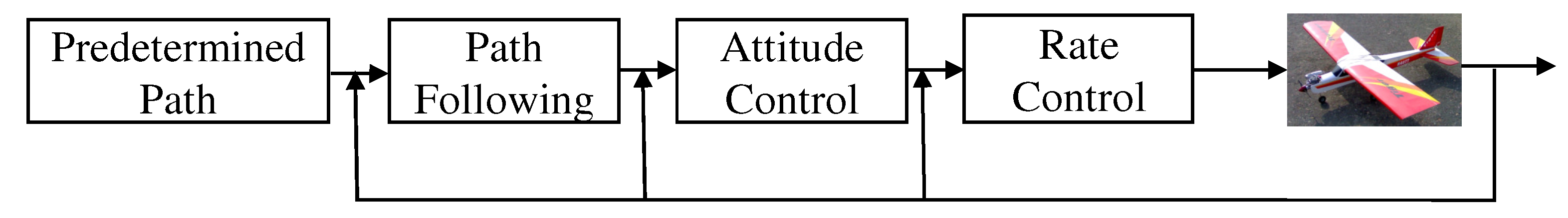
1. Introduction

Unmanned aerial vehicles (UAVs) are widely used by military and civilian industries in a huge number of applications such as aerial surveillance and photography and payload deployment [1]. However, with low-cost sensors and electronics, there is a significant interest in using low-cost UAVs among aircraft hobbyists, academic researchers, and industrials. To improve the usage of UAVs in all applications, the ability of the UAV to precisely follow a predetermined path must be considered. For small UAVs, the internal disturbances such as unmodeled dynamics, model uncertainties, and parameter perturbation in addition to external disturbances, such as gust and turbulence, make the design of the flight control system more difficult. Effective path tracking strategies must be accurate and robust to overcome these challenges.

The concept of the trajectory tracking problem is to force the vehicle to be in a certain location at a certain time. In a gusty environment or if the external disturbances are not controlled, the vehicle will oscillate around the desired location. Instead of trajectory tracking approach, many researchers adopt path following algorithms to force the vehicle to follow the path rather than going directly to the next waypoint at a specific time. In other words, the difference between the trajectory tracking approach and the path following algorithm is that the latter is time-independent [2,3].

Diverse path following algorithms have been successively implemented for real flight tests. There are two categories for path following algorithms, one is based on control theories while the other is based on a geometric interpretation [4,5]. Path following based on the geometric techniques generates guidance command based on the graphical derivation of the desired law. Geometric algorithms are easy for implementation and simple for understanding rather than the control techniques. It includes the pure pursuit guidance law [6], Line of Sight (LOS) guidance law [7], Nonlinear Guidance Law (NLGL) [8], Vector Field-based path following (VF) [1], and carrot chasing path following algorithm [9,10]. In most cases, as used in this paper, a combination of the pure pursuit guidance law and the LOS guidance law are considered. On the other hand, path following based on control techniques are common in applications because it guarantees system robustness to wind disturbances. A common control path following algorithm is based on proportional-integral-derivative (PID) control [11]. Rhee and Park [12] proposed a modified PID controller with feedforward ability to improve the performance of path following. Gain scheduling approach is also used for trajectory tracking by generating integrated guidance and control algorithms for autonomous vehicles [13]. Linear Quadratic Regulator based path following (LQR) [14] is also a well-known control technique used for UAV path following.

The path-following algorithms based on CC uses a virtual target point (VTP) on the path. The guidance laws directly guide the vehicle to chase the virtual point; meanwhile, the vehicle will ride the path. The distance between the VTP and the UAV position projected on the path is often called virtual distance. The selection criteria of the virtual track distance parameter is a trade-off in which the stability of the generated guidance laws is directly affected by its location [15].

The combination of pure pursuit and line of sight-based path following (PLOS) is a geometric technique for generating guidance law. The pure pursuit guidance law guides the UAV to the following waypoint, while the LOS guidance law directs the vehicle to ride the LOS. The weighting sum of both guidance laws forces the UAV to slide on the path to the consequent waypoint [16].

In this research, guidance commands for the UAV orientation are generated using carrot chasing and PLOS with a receding virtual waypoint. The UAV can alter its heading by changing the attitude. The nonlinear flight control system shown in Figure 1 highlights the sequence of generating physical control surface commands starting with a predefined path, followed by generating the desired guidance command. The control law is designed based on the two-timescale separation concept, which is discussed in the following [17].

For decades, automatic control occupies increasingly a significant place in aeronautics; many works discuss various aspects related to the control systems automation. The purpose of the controller is to ensure that the output closely tracks the input while optimizing the controller parameters for achieving the best performance, focusing on the responsibilities of the controller to calculate the control commands while keeping the system overshoot, settling time, and steady-state error within defined design margins based on the system requirements. In addition, to meet increasing demands on performance and reliability of UAVs, nonlinear control techniques are often utilized. These techniques are actively being studied to handle nonlinear aerodynamics and kinematic effects, actuator saturation, rate limitations, modeling uncertainty, and time-varying dynamics [6].

Typical linear flight control systems are designed based on linear design models that capture the approximate motion of the system under specific scenarios. Yamasaki [11] assumed the longitudinal dynamics are decoupled from the lateral-directional dynamics and utilized successive loop closure. However, a problem of this approach is that good performance and robustness properties cannot be guaranteed for a highly nonlinear fighter aircraft. Moreover, there are many hard nonlinearities such as saturation, dead-zones, and backlash whose discontinuous nature does not allow linear approximation, hence cannot be analyzed using linear analysis tools.

Nonlinear control methods have been developed to overcome the shortcomings of linear design approaches. NLDI approach is one of the best known and has been used successfully to address some practical control problems, as it is based on algebraically transforming a nonlinear system dynamic into a fully or partly linear one so that linear control techniques can be applied. It differs from the conventional linearization using Jacobian technique [18], which is achieved by exact state transformation and feedback under the assumption of a correct onboard dynamic model, instead of a linear approximation of the dynamics around trim points [17]. However, there are also a number of important shortcomings and limitations associated with NLDI approach as it is model-dependent flight controller [17,19]. In aircraft flight control, the aerodynamic forces and moments acting on the aircraft are important sources of nonlinearity to be dealt with. In practice, these cannot be modeled exactly and, hence, perfect cancellation is not possible. Consequently, it still has fatal limitations associated with the exact states feedback linearization especially in the case of unmodeled dynamics and parameter uncertainties. Unfortunately, the accurate knowledge of the nonlinear system dynamics is unavailable, which degrades the robustness of the designed controller using NLDI, as it is sensitive to any small perturbations in the system model. Consequently, a modification on the NLDI is required to degrade the model dependency of the flight controller.

Based on the literature, a robust UAV flight control methodology is still required to track a severe acute maneuver command with the existence of external disturbance and model uncertainties. For this objective, the main contribution of the current research is to design a fully autonomous guidance and control algorithm by combining simple geometric path following guidance law and a modified NLDI flight controller in one control algorithm. The key contributions of this paper are summarized as follows:

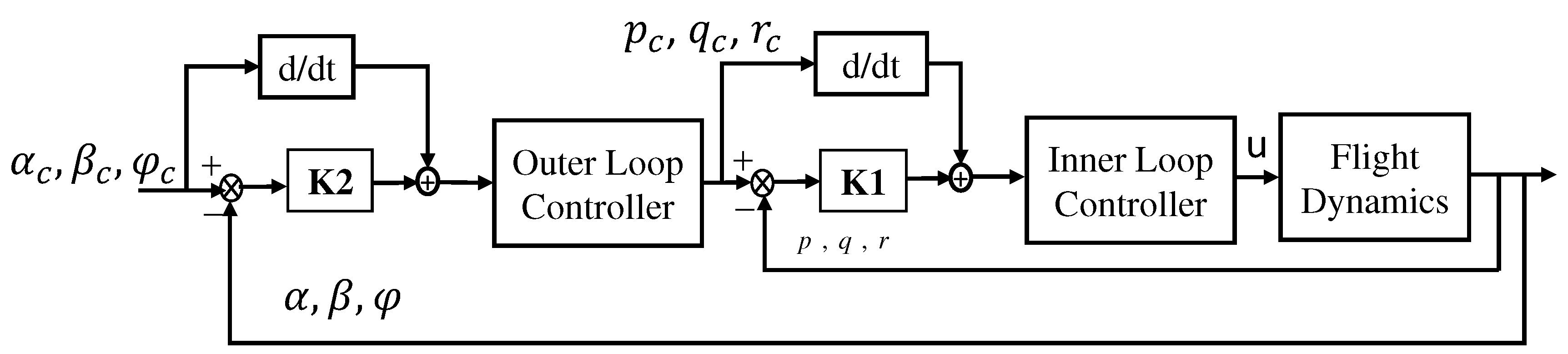
• Feedback linearization approach is employed to achieve the best UAV maneuvers. The most inner loop is the fastest dynamics corresponding to the angular rate states p, q, and r, which are controlled by three inputs: aileron, elevator, and rudder deflections. The consequent outer states $\alpha$, $\beta$, and $\mu$ are slower than the previous loop, which are controlled by angular rate states p, q, and r. The designed control law guarantees asymptotic stability of the error between the desired states and the current one. The premise of this approach is that there is a significant execution time between the inner fast states and the outer slow states in the open-loop plant.
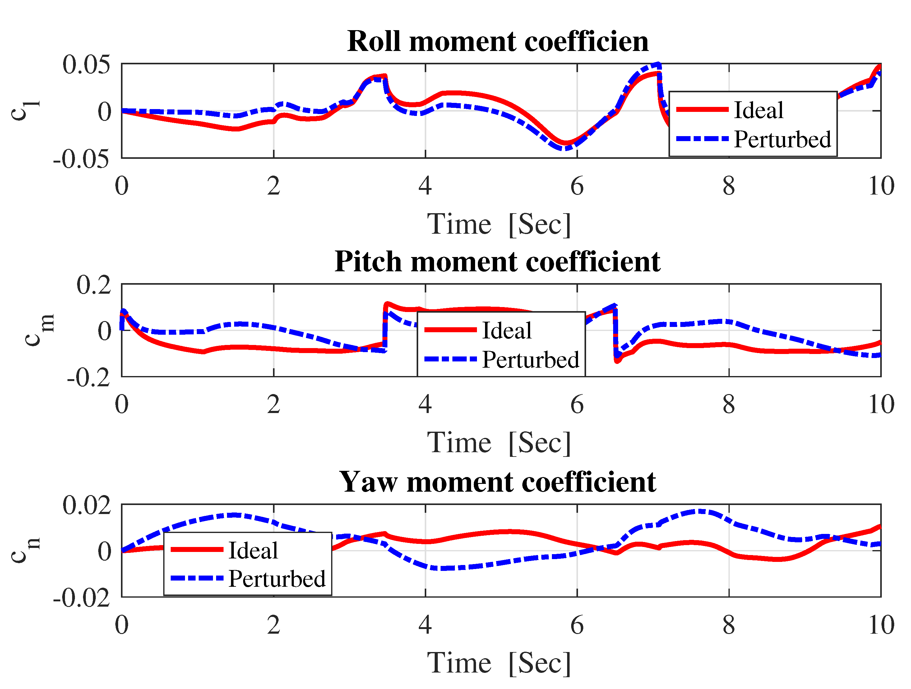
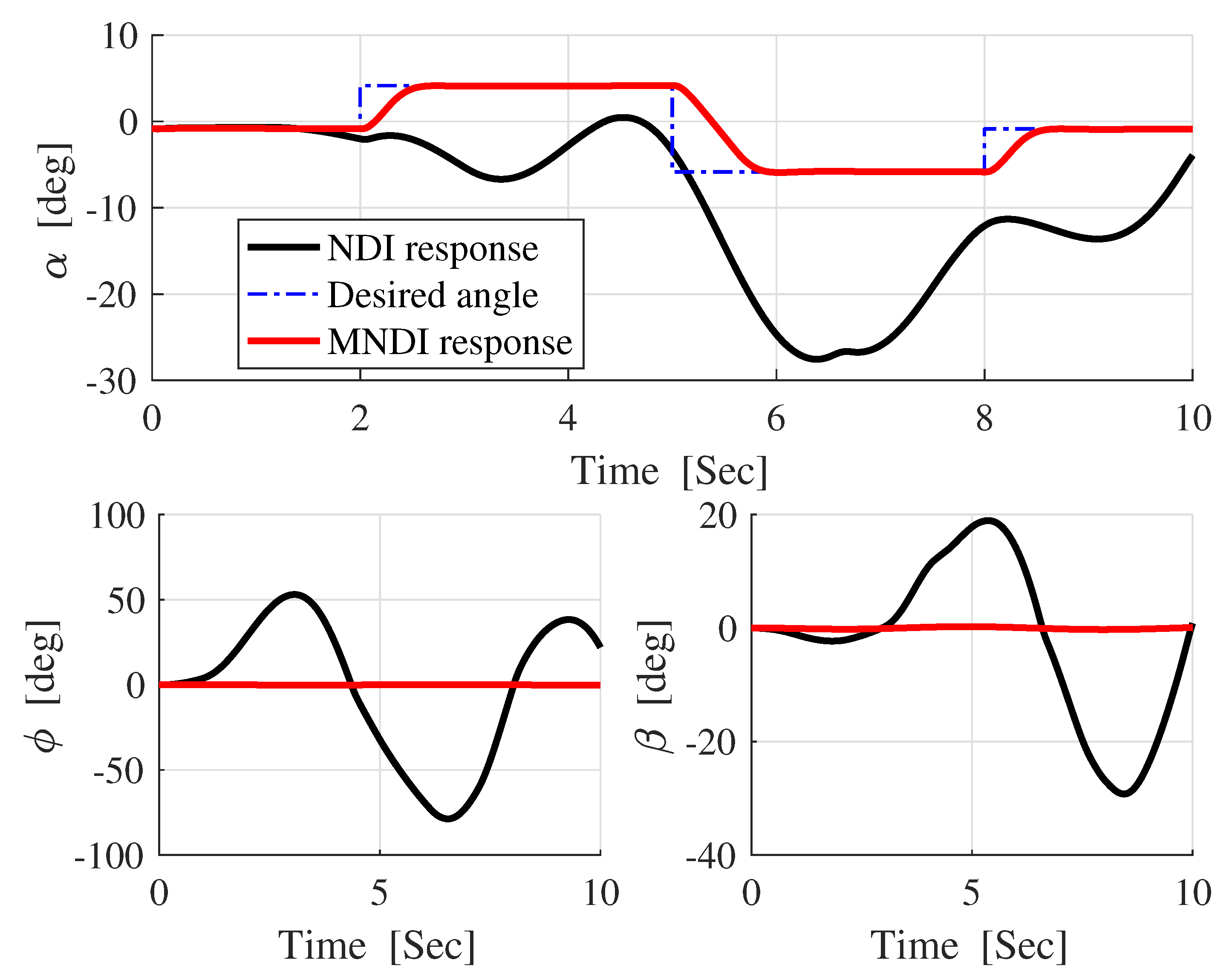
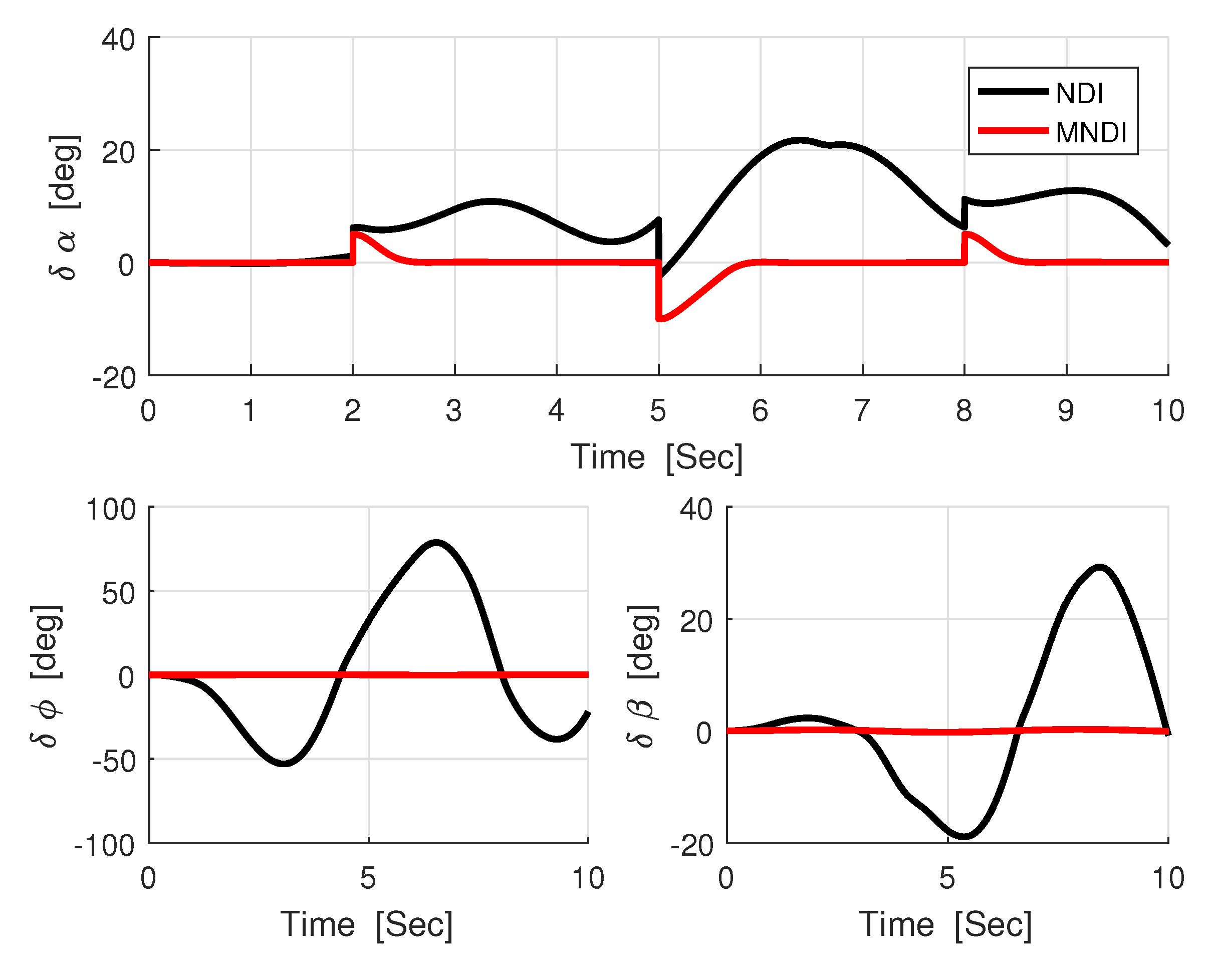
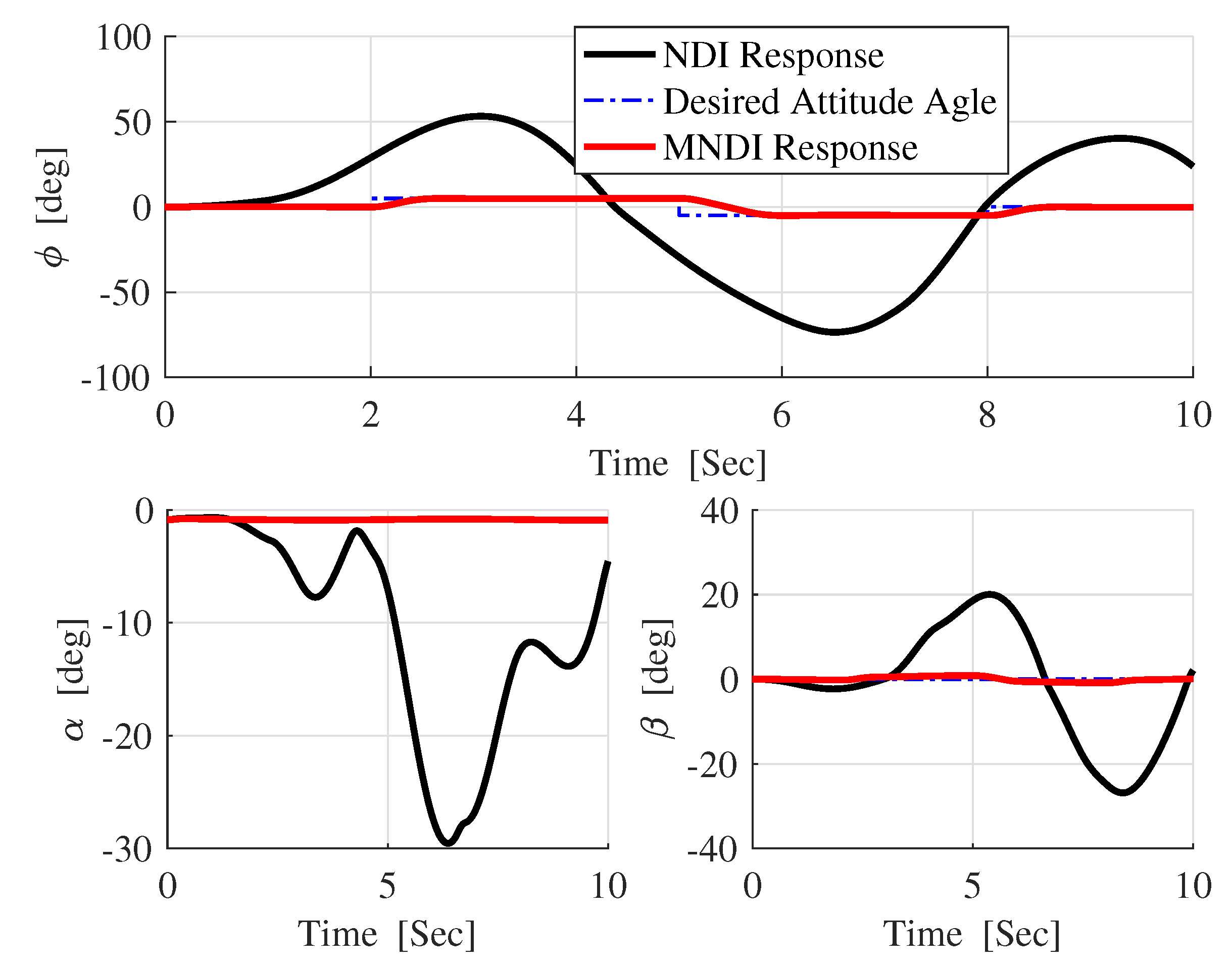
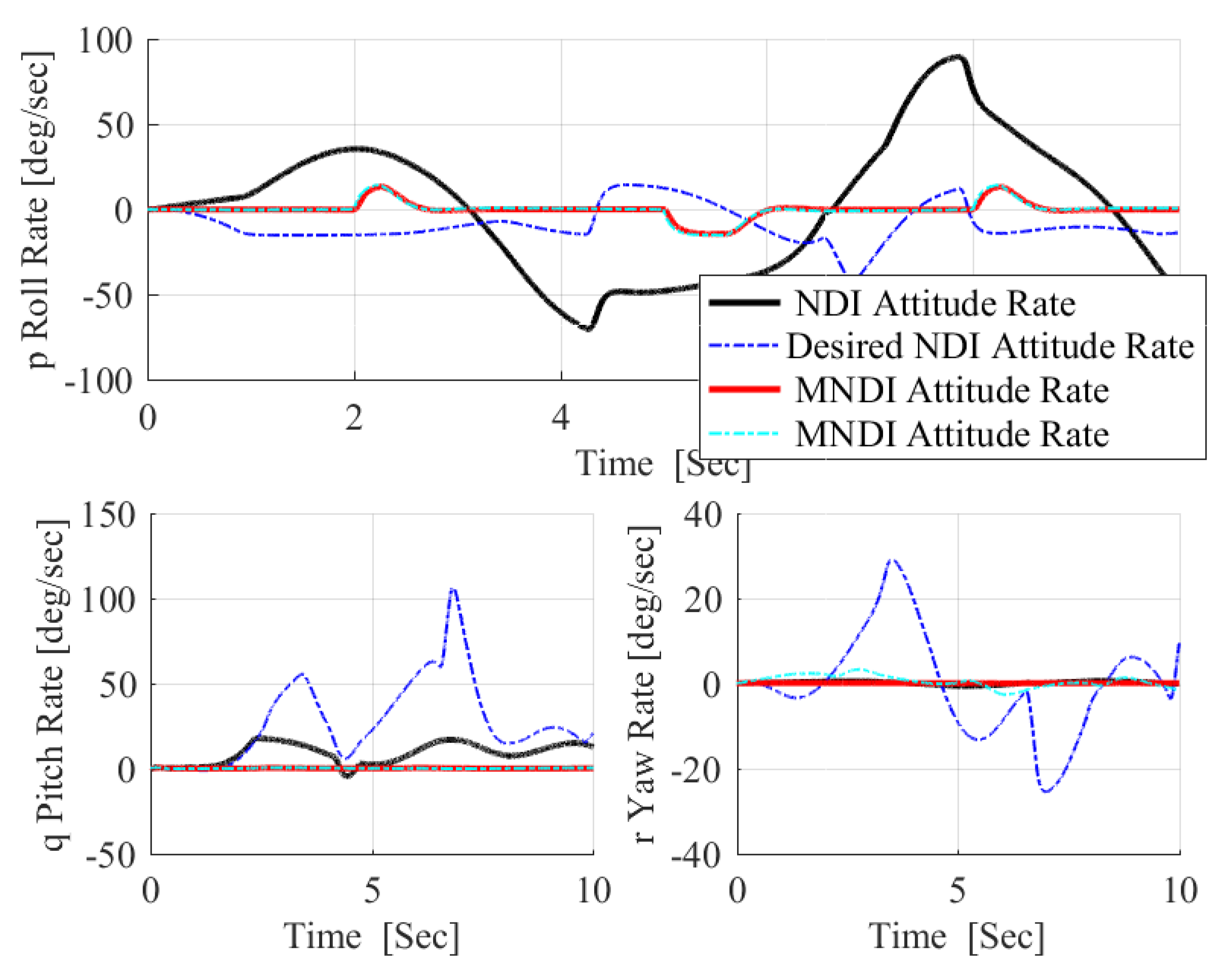
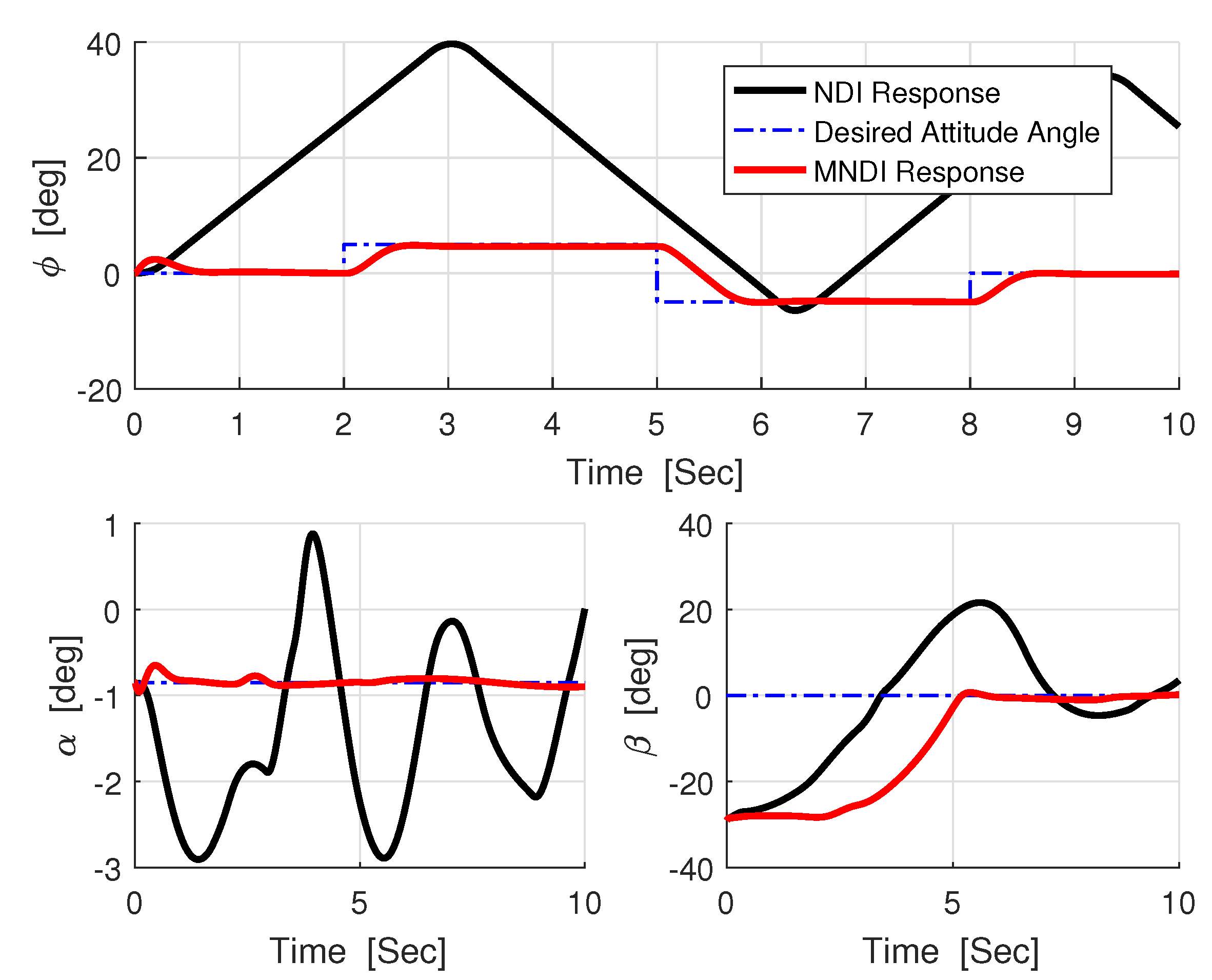
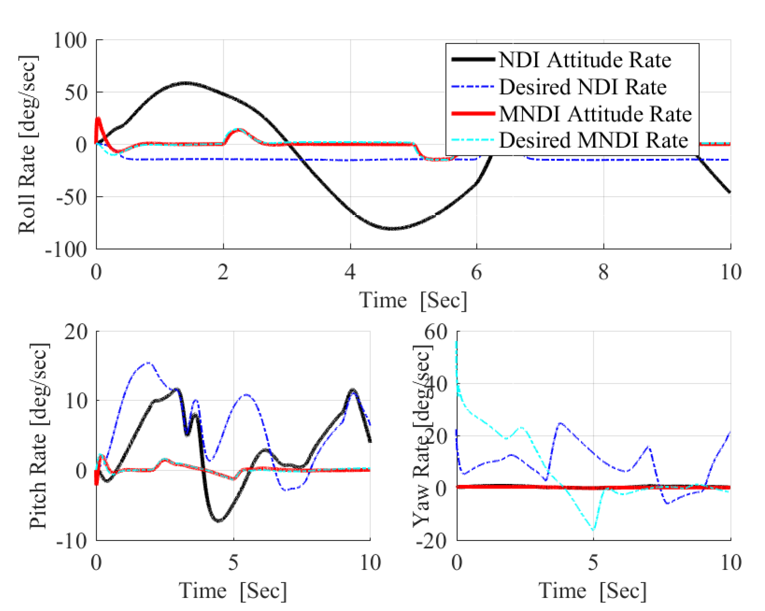
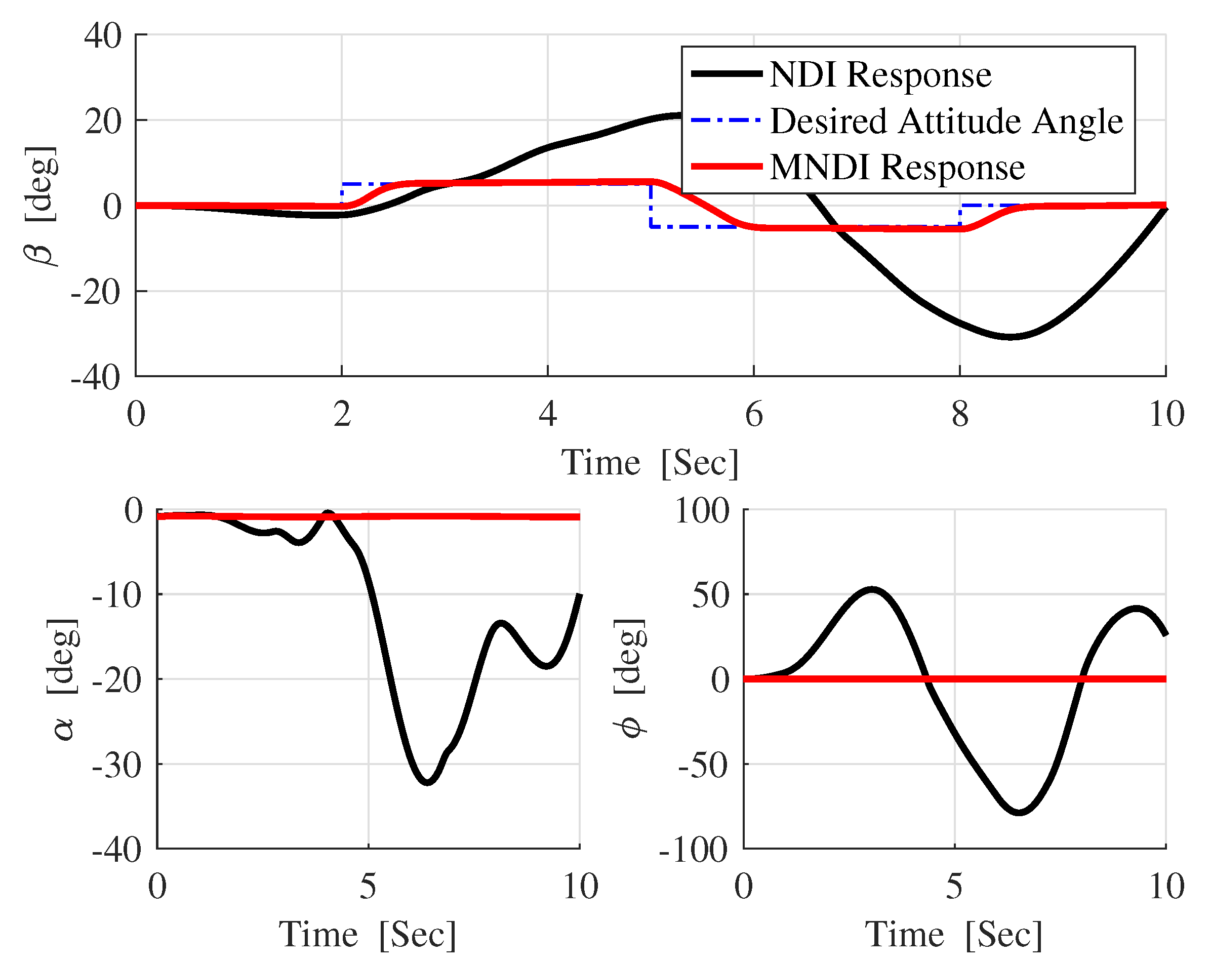
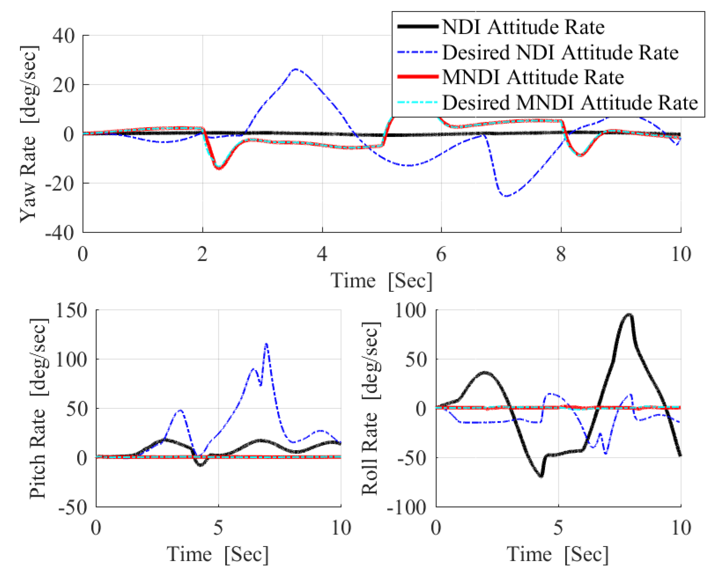
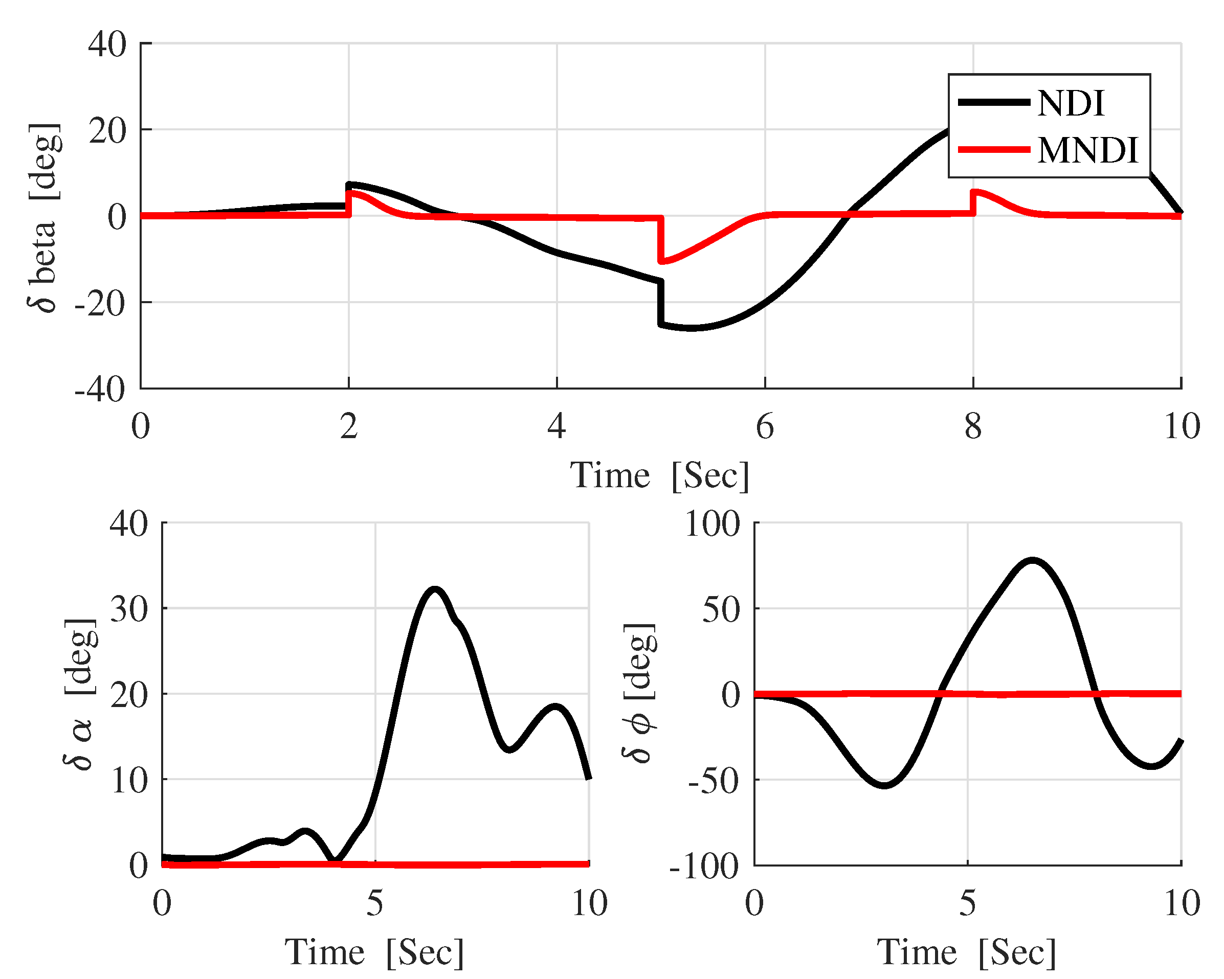
• The most critical task for the flight control system is to maintain flight stability under uncertainties and perturbed conditions. In fixed-wing UAV system, altitude and attitude angles $\varphi$, $\theta$, and $\psi$ are playing a vital role for flight stabilization. However, NLDI is a model-dependent flight controller, which means it is prone to any small system variations. In this paper, a new modification on NLDI incorporates all uncertainties that increases the system robustness against the model mismatch.
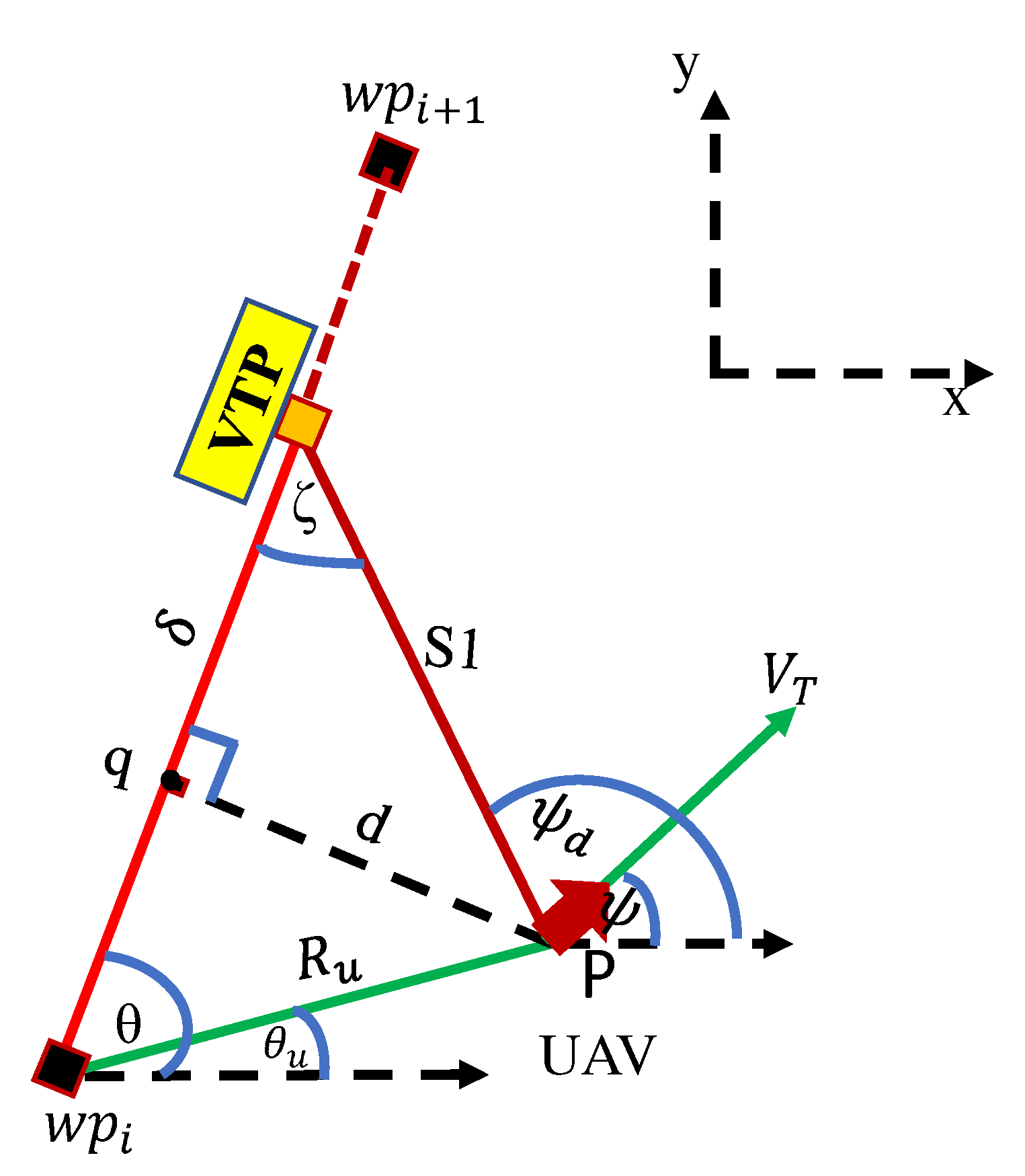
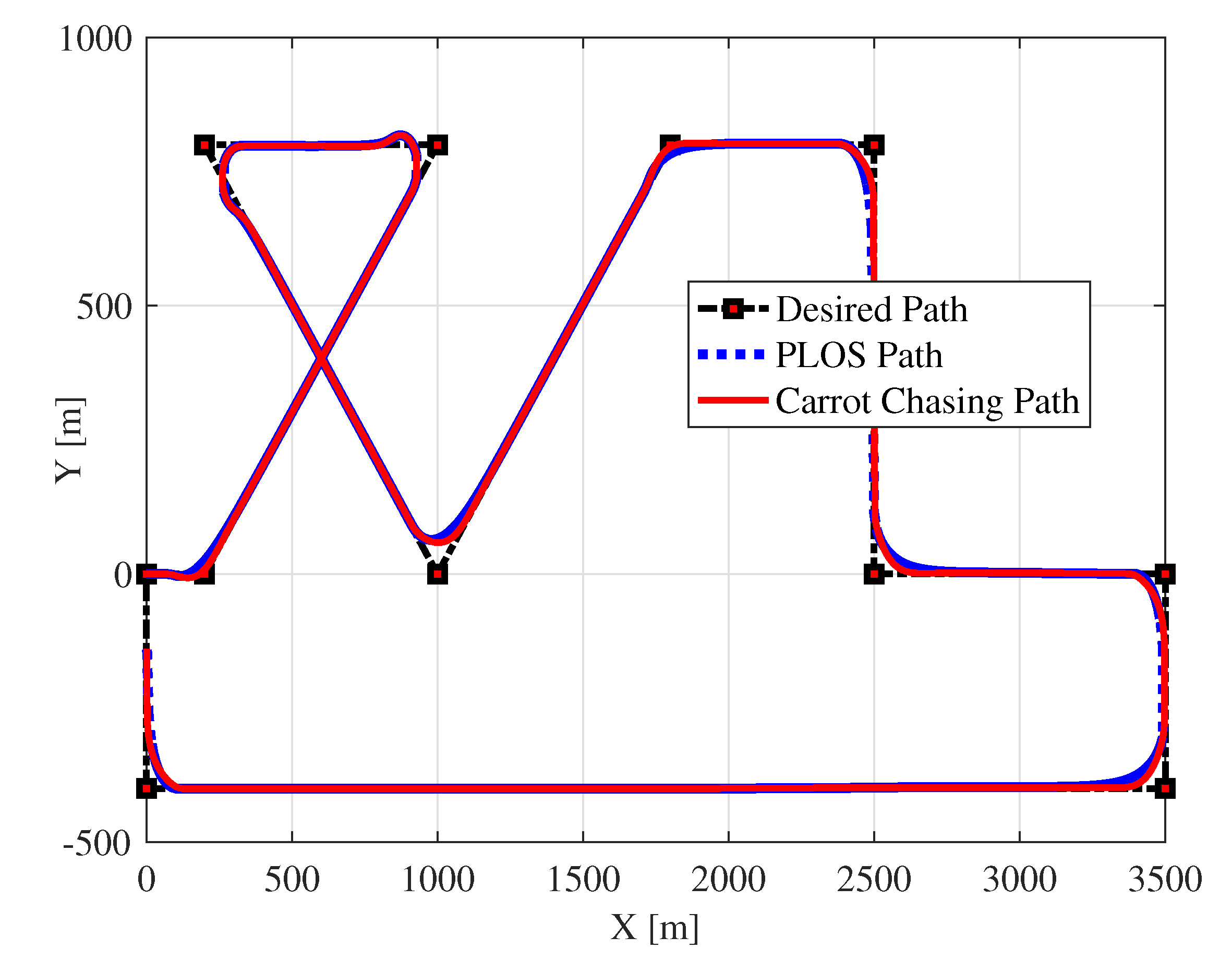
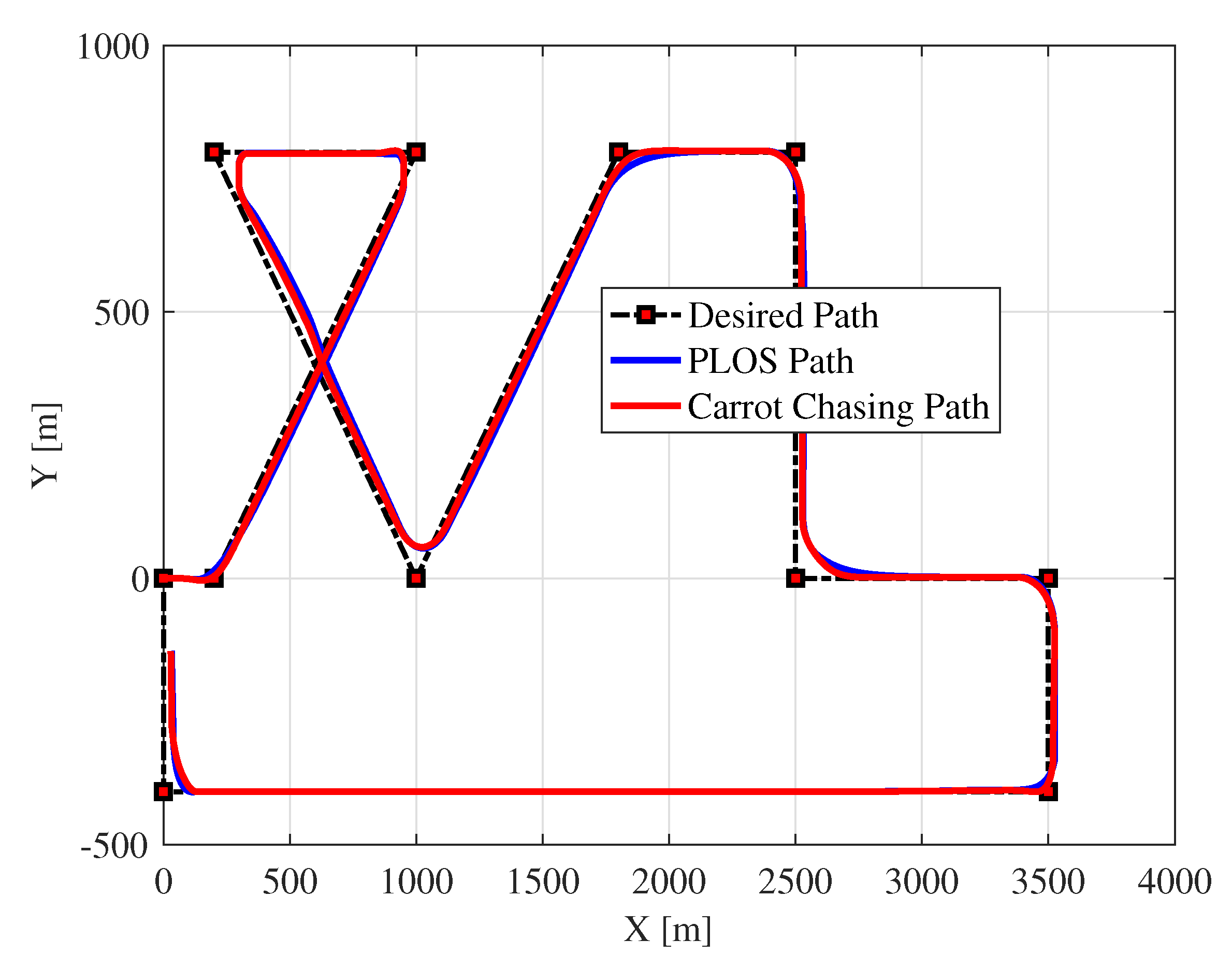
• The study presented in this research is to compare and analyze two common paths following algorithms for UAV. The concept of path following based on carrot chasing is to track a virtual target point sliding along the line of sight between two consequent waypoints. After each time updating, the UAV gets closer to the path and asymptotically follows the path. On the other hand, the concept of Pure pursuit and line-of-sight (PLOS) path following algorithm vanishes the cross-track error distance using LOS control law, in addition to eliminating the LOS angle error using pure pursuit guidance law.

The paper is structured as follows. Section 2 presents the path following formulation. The UAV is directed to its heading by altering its attitudes. Section 3 discusses the derivation of the control law using NLDI. The modified NLDI (MNLDI) control law is derived in Section 4. Simulation results are presented in Section 5. Finally, the conclusions of this paper are given in Section 6.

2. Guidance Law Formulation

The high rate of increasing of UAV industrial applications has resulted in highly complex missions. Consequently, adopting suitable path-following algorithms guarantees stable platforms that meet the desired performance criteria. Since the path following for most UAVs depends on the correction of the tracking error, these systems present the difficulty of following in large tracking-error situations, e.g., steep curved path following or tracking under wind turbulence. This might cause control saturation or divergence because the control command tends to increase as the tracking error becomes large [6]. Carrot chasing path following algorithm is easy to implement as it demands only one gain-tuning. It produces guidance commands that are not large, with no relation to tracking error quantities but relating to LOS angle. However, the simulation results show that it is not robust in the windy fields. The combination of pursuit and LOS guidance law is intuitive and easy for implementations. Although it is robust against wind disturbances, it is sensitive to variation to its gains.

2.1. Problem Description

The initial position of the UAV is $p(x_p,y_p,h_p)$ with the actual heading angle $\psi$. Since the objective is to be on the path, the demanded heading angle ${\psi }_d$ guides the UAV to follow the path. Figure 2 shows two waypoints $W{p}_i$ and $W{p}_{i+1}$, with LOS angle $\theta$. The cross-track error d is a measure of the normal distance from the path. The main task of the path following algorithm is to minimize ($d\to 0$ and $\psi -\theta \to 0$) as ($t\to \infty$), as given in the cost function (1).

$$\begin{array}{c}\hfill \underset{t\to \infty }{min}(d,\psi -\theta )\end{array}$$

(1)

2.2. Carrot Chasing Guidance Algorithm

In this algorithm, it is assumed there is a virtual point sliding along the path and the UAV is allowed to chase it. Gradually, the UAV is directed toward the path and asymptotically ride it. The VTP is called the carrot and the UAV chases the carrot. The designed algorithm has three steps: first, calculating the cross-track error d, then the location of the VTP is updated and, finally, producing the guidance command. Assume the UAV is at location p with the current heading angle $\psi$. The perpendicular distance from the actual position of the UAV to the path is the cross-track error d. To compensate for the LOS angle and cross-track error distance, the subsequent stepwise Pseudo code is followed [15]:

• Initialize the waypoints $\to W_i=(x_i,y_i,h_i)$, $W_{i+1}=(x_{i+1},y_{i+1},h_{i+1})$, UAV current position $p=(x_p,y_p,h_p)$, and the path parameter $\delta$.
• Calculate the LOS angle $\to \theta =atan2((y_{i+1}-y_i),(x_{i+1}-x_i))$.
• Calculate the angle between the current position p and the previous waypoint $W{p}_i$ $\to {\theta }_u=atan2((y_p-y_i),(x_p-x_i))$.
• Calculate the distance between the current position p and the next waypoint $W{p}_i$$\to R_u=\sqrt{{(x_p-x_i)}^2+{(y_p-y_i)}^2}$.
• Calculate the distance between the UAV current position p and the VTP $\to S_1=\sqrt{{\delta }^2+{(R_{u}sin(\theta -{\theta }_u))}^2}$.
• Calculate the cross-track error angle $\to \zeta =asin(R_{u}sin(\theta -{\theta }_u)/S_1)$.
• Calculate the desired heading angle $\to {\psi }_d=\zeta +\theta$.
• Calculate the current miss distance S according to desired waypoint radius r$\to S=\sqrt{{(y_{i+1}-y_i)}^2+{(x_{i+1}-x_i)}^2}\le r$.
• Calculate the desired guidance law $\to {\varphi }_c=k\left({\psi }_d-\psi \right)V_a$, which represents the desired bank angle for UAV with airspeed $V_a$.

The UAV location is updated based on the desired waypoint radius r and the current UAV miss distance S while the performance of following the path is directly depending on the assumed path parameter $\delta$. For low $\delta$, the UAV is directed toward the desired path, therefore an overshoot is carried out. Consequently, the UAV oscillates around the desired path, hence the settling time will be increased. By increasing the path parameter $\delta$, the UAV will settle on the path quickly.

2.3. Pure Pursuit and LOS Guidance Algorithm

The combination of pure pursuit and line of sight-based path following (PLOS) is a geometric technique for generating guidance law. The pure pursuit guidance law drives the UAV to the next waypoint, while the LOS guidance law steers the vehicle to toward the LOS. The guidance law of the pure pursuit is given in Equation (2), where $k_1$ is a positive constant gain empirically determined such that the UAV path is smoothly parallel to the LOS path.

$$\begin{array}{c}\hfill {\psi }_p=k_1\left(\theta -\psi \right)\end{array}$$

(2)

Another LOS guidance law is given in Equation (3), where $k_2$ is a constant selected to attract the UAV to be on the desired path.

$$\begin{array}{c}\hfill {\psi }_{LOS}=k_{2}d\end{array}$$

(3)

The PLOS guidance command for straight-line path following is a combination of both guidance laws in Equation (2), which is outlined in the following stepwise Pseudo code.

• Initialize the waypoints vector $\to W_i=(x_i,y_i,h_i)$, $W_{i+1}=(x_{i+1},y_{i+1},h_{i+1})$, UAV current position $p=(x_p,y_p,h_p)$, and the path parameter $\delta$.
• Calculate the LOS angle $\to \theta =atan2((y_{i+1}-y_i),(x_{i+1}-x_i))$.
• Calculate the distance between the current position p and the next waypoint $W{p}_i$$\to R_u=\sqrt{{(x_p-x_i)}^2+{(y_p-y_i)}^2}$.
• Calculate the cross-track error distance $\to d=R_{u}sin(\theta -{\theta }_u)$.
• Calculate the current miss distance S according to desired waypoint radius r$\to S=\sqrt{{(y_{i+1}-y_i)}^2+{(x_{i+1}-x_i)}^2}\le r$.
• Calculate the desired guidance law $\to {\varphi }_c=k_1\left(\theta -\psi \right)+k_{2}d$, which represents the desired bank angle.

3. Nonlinear Dynamic Inversion Control Law

NLDI is a control strategy that uses the model of a system to control it and through that eliminates the need for gain scheduling and improves performance. Consequently, NLDI controller is used for achieving high maneuverability associated with a high level of accuracy [6]. The attitude control is generally conducted using two loops: the first rotation control loop for fast-timescale state dynamics, and attitude control loop for slow-timescale state dynamics. The two-timescale NLDI approach used to achieve the desired angle of attack, side-slip angle and the desired bank angle $({\alpha }_c,{\beta }_c,{\varphi }_c)$ are shown in Figure 3, which reduces the controller order to simplify the design process [20].

The inner loop corresponds to the fast state dynamics roll, pitch and yaw angular rates ($p,q,r$), which are controlled by control surface commands aileron, elevator, and rudder ($u={[{\delta }_a,{\delta }_e,{\delta }_r]}^T$), respectively. The outer loop corresponds to the slow-state dynamics ($\alpha ,\beta ,\varphi$), which are controlled by angular rates ($p,q,r$). Regarding the outer loop, the transient dynamics of the fast states occur quickly so that they have a negligible effect on the slow states. In the inner loop process, slow-timescale variables are assumed to remain constant. The fast loop controller attempts to track the desired angular rates ($p_c,q_c,r_c$).

3.1. Inner Fast Loop

The most inner fast loop dynamic states ($p,q,r$) are controlled by the control surfaces commands (${\delta }_a,{\delta }_e,{\delta }_r$). The angular rate dynamic inversion is derived from the moment in Equation (4) of the Tiger-Trainer (a small commercial off-the-shelf Radio-Controlled) airplane model is given in [21] by solving for the control surface commands.

$$\begin{array}{cc}\hfill {\mathbf{I}}_B{\dot{\overrightarrow{\omega }}}_B& ={\overrightarrow{\omega }}_B\times {\mathbf{I}}_B{\overrightarrow{\omega }}_B+{\overrightarrow{M}}_B\hfill \end{array}$$

(4)

where the body fixed rotational rates ${\overrightarrow{\omega }}_B={[p,q,r]}^T$, and ${\mathbf{I}}_B={[I_x,I_y,I_z,I_{xz}]}^T$ is the moment of inertia matrix. The total body coordinate system’s moments ${\overrightarrow{M}}_B={[l,m,n]}^T$ are composed partially by moments generated by the aerodynamics of the air-frame $M_a$ and partially by moments generated by the control surface deflections $M_c$. The moment equation is given in Equation (5).

$$\begin{array}{cc}\hfill {\mathbf{I}}_B{\dot{\overrightarrow{\omega }}}_B& ={\overrightarrow{\omega }}_B\times {\mathbf{I}}_B{\overrightarrow{\omega }}_B+{\overrightarrow{M}}_a+{\overrightarrow{M}}_c\delta \hfill \end{array}$$

(5)

Applying NLDI to Equation (5) results in an expression for the control surface deflections $u={[{\delta }_a,{\delta }_e,{\delta }_r]}^T$, which is given in Equation (6).

$$\begin{array}{c}\hfill {[{\delta }_a,{\delta }_e,{\delta }_r]}^T={\overrightarrow{M}}_c^{-1}\left[{\mathbf{I}}_B\nu -{\overrightarrow{\omega }}_B\times {\mathbf{I}}_B{\overrightarrow{\omega }}_B-{\overrightarrow{M}}_a\right]\end{array}$$

(6)

where $\nu ={[{\nu }_p,{\nu }_q,{\nu }_r]}^T$ are the designed control laws for roll, pitch, and yaw angular rates, respectively, given in Equations (7)–(9).

$$\begin{array}{cc}\hfill {\nu }_p& ={\dot{p}}_c-K_p(p-p_c)\hfill \end{array}$$

(7)

$$\begin{array}{cc}\hfill {\nu }_q& ={\dot{q}}_c-K_q(q-q_c)\hfill \end{array}$$

(8)

$$\begin{array}{cc}\hfill {\nu }_r& ={\dot{r}}_c-K_r(r-r_c)\hfill \end{array}$$

(9)

where ($p_c,q_c,r_c$) are the desired angular rates with their derivatives (${\dot{p}}_c,{\dot{q}}_c,{\dot{r}}_c$), and ($K_p,K_q,K_r$) are constant positive gains represent the bandwidth frequencies of the control signals in the roll, pitch, and yaw channels, respectively. The gains are set as high as possible without exciting structural modes or being subjected to the bandwidth limitations of the control actuators. The designed control law guarantees the global asymptotic stability of the system i.e., the error difference between the desired angular rate and the actual one will exponentially decay to zero for any initial conditions. Assuming the error ($e_p=p-p_c,e_q=q-q_c,e_r=r-r_c$), then from Equations (7)–(9), the error vector is given in Equations (10)–(12)

$$\begin{array}{c}\hfill {\dot{e}}_p+K_p{e}_p=0\end{array}$$

(10)

$$\begin{array}{c}\hfill {\dot{e}}_q+K_q{e}_q=0\end{array}$$

(11)

$$\begin{array}{c}\hfill {\dot{e}}_r+K_r{e}_r=0\end{array}$$

(12)

The frequencies of the roll, pitch, and yaw channels are set to ($K_p=K_q=K_r=50$ Hz) to ensure the avoidance of coupling between the inner loop and the outer loop. Continuously increasing the frequencies will increase the rate of error decaying, which considering the channel’s frequencies rise, will result in the higher coupling effect in the lateral plane between the roll and yaw states.

3.2. Outer Slow Loop

The outer slow loop dynamic states ($\alpha ,\beta ,\varphi$) are controlled by the most inner loop states ($p,q,r$). The outer slow loop control laws are designed based on performing the slow response of the outer loop by exciting the fast dynamic loop. A fast-transient response is assumed so that they have a negligible effect on the slow states. The differential equations governing the variation in time of the controlled variables $\alpha$, $\beta$, and $\varphi$ are obtained by differentiation of the aerodynamic angles given in Equations (13) and (14) and the Tiger-Trainer UAV attitude equation given in [21], respectively.

$$\begin{array}{c}\hfill \alpha =atan2(w,u)\end{array}$$

(13)

$$\begin{array}{c}\hfill \beta =atan2(v,V_a)\end{array}$$

(14)

where the body fixed velocity components are ($u,v,w$), and $V_a$ is the UAV airspeed. The equations relating the derivatives of the aerodynamic angles with the angular rates ($p,q,r$) are given in Equations (15)–(17).

$$\begin{array}{cc}\hfill \dot{\alpha }& =q-(pcos\alpha +rsin\alpha )tan\beta +\frac{Zcos\alpha -(X+T)sin\alpha +F_{\alpha g_b}}{m{V}_{a}cos\beta }\hfill \end{array}$$

(15)

$$\begin{array}{cc}\hfill \dot{\beta }& =psin\alpha -rcos\alpha +\frac{Y-Tcos\alpha sin\beta +F_{\beta g_b}}{m{V}_a}\hfill \end{array}$$

(16)

$$\begin{array}{cc}\hfill \dot{\varphi }& =p+qtan\theta sin\varphi +rtan\theta cos\varphi \hfill \end{array}$$

(17)

where T is the engine thrust, $X,Y,Z$ are the aerodynamic forces in body axes, m is the UAV mass, and $F_{\alpha g_b},F_{\beta g_b}$ are the gravitational forces in body axes. Applying NLDI to the attitude Equations (15)–(17) results in an expression for the desired angular rates ${[p_c,q_c,r_c]}^T$ as given in Equation (18), which is the desired input for the most inner loop.

$$\begin{array}{c}\hfill \left[\begin{array}{c}{p}_c\\ q_c\\ r_c\end{array}\right]=g^{-1}\left(\left[\begin{array}{c}{\nu }_{\alpha }\\ {\nu }_{\beta }\\ {\nu }_{\varphi }\end{array}\right]-\left[\begin{array}{c}{F}_{\alpha }\\ F_{\beta }\\ 0\end{array}\right]\right)\end{array}$$

(18)

where g is a square matrix given in Equation (19) that relates the required angular rates $p_c,q_c,r_c$ with the desired attitudes rate. ${\nu }_{\alpha },{\nu }_{\beta },{\nu }_{\varphi }$ are the designed control laws for ($\alpha ,\beta ,\varphi$) and are given in Equations (20)–(22).

$$\begin{array}{c}\hfill g=\left(\begin{array}{ccc}-cos\alpha tan\beta & 1& -sin\alpha tan\beta \\ sin\alpha & 0& -cos\alpha \\ 1& tan\theta sin\varphi & tan\theta cos\varphi \end{array}\right)\end{array}$$

(19)

$$\begin{array}{cc}\hfill {\nu }_{\alpha }& ={\dot{\alpha }}_c-K_{\alpha }(\alpha -{\alpha }_c)\hfill \end{array}$$

(20)

$$\begin{array}{cc}\hfill {\nu }_{\beta }& ={\dot{\beta }}_c-K_{\beta }(\beta -{\beta }_c)\hfill \end{array}$$

(21)

$$\begin{array}{cc}\hfill {\nu }_{\varphi }& ={\dot{\varphi }}_c-K_{\varphi }(\varphi -{\varphi }_c)\hfill \end{array}$$

(22)

where (${\alpha }_c,{\beta }_c,{\varphi }_c$) are the desired attitude angles with their derivatives (${\dot{\alpha }}_c,{\dot{\beta }}_c,{\dot{\varphi }}_c$), and ($K_{\alpha },K_{\beta },K_{\varphi }$) are constant positive gains set to be $10\left[\mathrm{Hz}\right]$ to ensure the avoidance of coupling between the outer loop and the inner loop. The designed control law guarantees the global asymptotic stability of the system, i.e., the error difference between the desired attitude angle and the actual one will exponentially decay to zero for any initial conditions. Assuming the errors are ($e_{\alpha }=\alpha -{\alpha }_c,e_{\beta }=\beta -{\beta }_c,e_{\varphi }=\varphi -{\varphi }_c$), then from Equations (20)–(22), the error vector is given in Equations (23)–(25).

$$\begin{array}{c}\hfill {\dot{e}}_{\alpha }+K_{\alpha }{e}_{\alpha }=0\end{array}$$

(23)

$$\begin{array}{c}\hfill {\dot{e}}_{\beta }+K_{\beta }{e}_{\beta }=0\end{array}$$

(24)

$$\begin{array}{c}\hfill {\dot{e}}_{\varphi }+K_{\varphi }{e}_{\varphi }=0\end{array}$$

(25)

As soon as the two control loops are designed with the desired inputs (${\alpha }_c$, ${\beta }_c$, ${\varphi }_c$) and the required control surfaces commands (${\delta }_a,{\delta }_e,{\delta }_r$), the flight control system is ready to track the desired trajectory. Therefore, the guidance law will be applied as a desired input for the outer dynamics control loop.

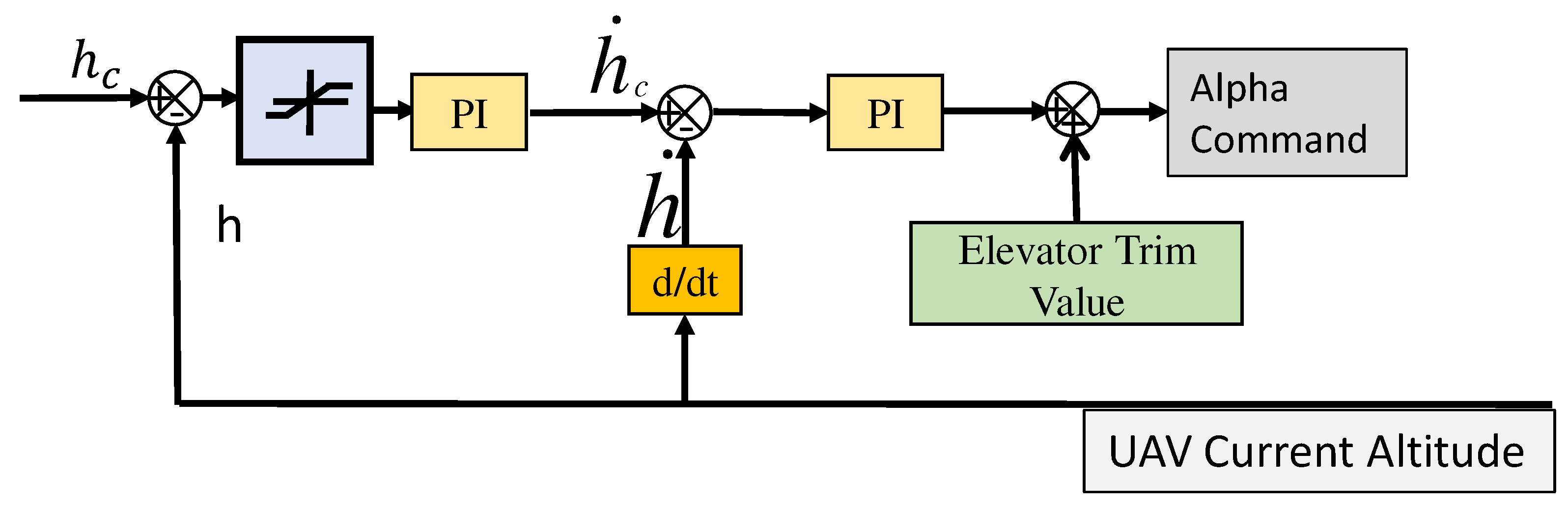
3.3. Altitude Control Loop

The altitude control loop is designed using a PI controller. The saturation limit is used to constrain the altitude error according to the flight envelope specification of Tiger-Trainer UAV model given in [21]. The classical PI controller is tuned offline with conventional tuning method [11], followed by fine-tuning to obtain the best tracking performances. The two cascaded PI controller is used to increase the robustness and to track the rate of change of climbing, as shown in Figure 4.

The altitude control loop equation is given in Equation (26) shows that the UAV altitude is controlled by executing a certain angle of attack. The error between the desired altitude and current altitude is controlled using PI controller.

$$\begin{array}{c}\hfill {\alpha }_c=(h_c-h)\left(k_{ph}+\frac{K_{ih}}{s}\right)+({\dot{h}}_c-\dot{h})\left(k_{p\dot{h}}+\frac{K_{i\dot{h}}}{s}\right)\end{array}$$

(26)

where $h_c$ is the desired altitude with its derivative ${\dot{h}}_c$, and h is the current altitude with its derivative $\dot{h}$.

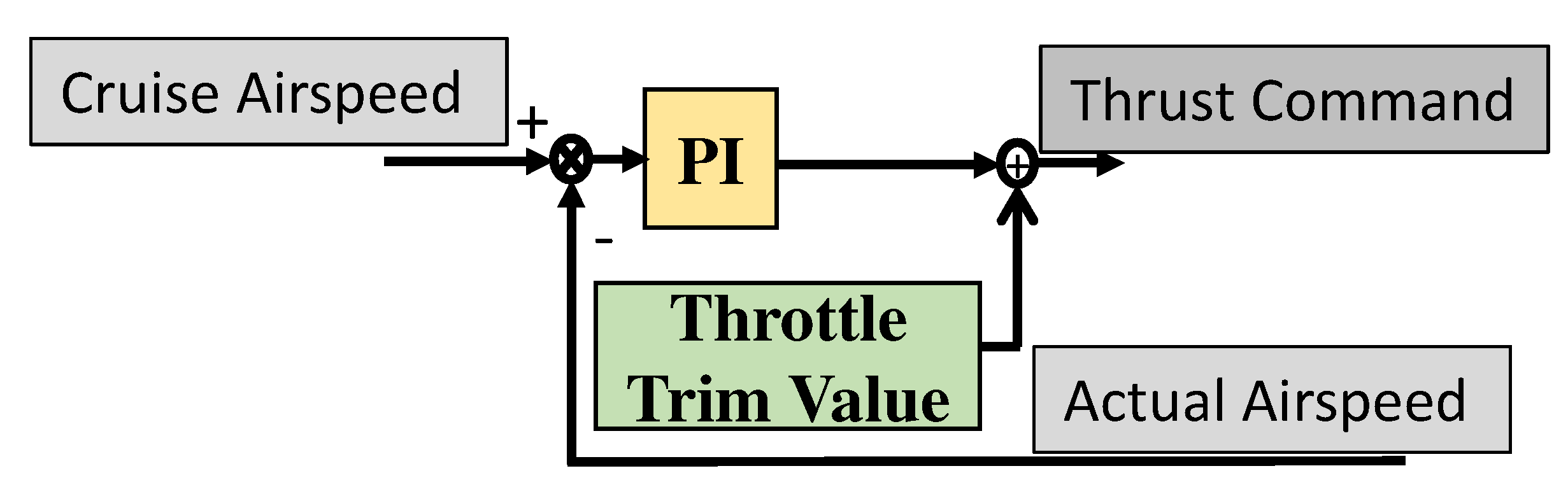
3.4. UAV Speed Control Loop

For strengthening the path-following ability of a UAV to keep tracking the desired position along the given required path, the UAV velocity holding must be taken into consideration. Applying a PI controller for the velocity error to get the desired thrust command ${\delta }_t$ given in Equation (27), the gains of PI controller are selected by trial and error to fulfill the accepted holding cruise speed, as illustrated in Figure 5.

$$\begin{array}{cc}\hfill {\delta }_t& =\left(k_p+\frac{K_i}{s}\right)\left(V_c-V_a\right)\hfill \end{array}$$

(27)

where $V_c$ is the desired cruise speed and $V_a$ is the current UAV airspeed.

4. Modified NLDI

The flight controller based on NDl provides the commanded control surface deflections as a function of the error of control variables. The complete deflection of the control surfaces is computed per each sampling time of the flight controller. In contrast, the flight controller based on the modified NLDI only computes the increments of control surface deflections by taking the influence of the acting control surface deflections into account. Consequently, the modified NLDI (MNLDI) is more robust against model mismatch than conventional NLDI. As a result, the attitude Equation (5) must be expanded to include the variation of the flight control command using a Taylor expansion. The approximated first-order attitude equation is given in Equation (28), in which only the first three terms are considered and the higher-order terms (H.O.T) are neglected.

$$\begin{array}{cc}\hfill {\mathbf{I}}_B{\dot{\overrightarrow{\omega }}}_B& \approx {\dot{\overrightarrow{\omega }}}_{B0}+{\left(\frac{\partial ({\overrightarrow{\omega }}_B\times {\mathbf{I}}_B{\overrightarrow{\omega }}_B+{\overrightarrow{M}}_a+{\overrightarrow{M}}_c\delta )}{\partial \omega }\left(\omega -{\omega }_0\right)\right)}_{{\delta }_0}+\hfill \\ \hfill & {\left(\frac{\partial ({\overrightarrow{\omega }}_B\times {\mathbf{I}}_B{\overrightarrow{\omega }}_B+{\overrightarrow{M}}_a+{\overrightarrow{M}}_c\delta )}{\partial \omega }\left(\delta -{\delta }_0\right)\right)}_{{\omega }_0}+H.O.T\hfill \end{array}$$

(28)

where ${\dot{\overrightarrow{\omega }}}_{B0}$ is the initial angular rates vector, and $\omega$ and $\delta$ are varying with time. The current control surface deflection command is the variation upon the previous control command. The moments generated by the control surface deflections $M_c$ are independent of $\omega$ and the aerodynamics moment $M_a$ is not a function of $\delta$. The (H.O.T) are small enough to be neglected, thus the approximated moment equation is given in Equation (29).

$$\begin{array}{cc}\hfill {\mathbf{I}}_B{\dot{\overrightarrow{\omega }}}_B& \approx {\dot{\overrightarrow{\omega }}}_{B0}+{\left(\frac{\partial ({\overrightarrow{\omega }}_B\times {\mathbf{I}}_B{\overrightarrow{\omega }}_B+{\overrightarrow{M}}_a)}{\partial \omega }\mathsf{\Delta }\omega \right)}_{{\delta }_0}+{\left(\frac{\partial \left({\overrightarrow{M}}_c\delta \right)}{\partial \delta }\mathsf{\Delta }\delta \right)}_{{\omega }_0}\hfill \end{array}$$

(29)

Furthermore, by assuming the deflection of control surfaces only generates a variation in moments, the variation in forces is small enough to be neglected. This assumption is reasonable for aircraft with traditional configuration, so that control surfaces are far from the aircraft center of gravity. Consequently, the second term of Equation (29) is negligible compared to the third term so the attitude equation is given in Equation (30).

$$\begin{array}{cc}\hfill {\mathbf{I}}_B{\dot{\overrightarrow{\omega }}}_B& \approx {\dot{\overrightarrow{\omega }}}_{B0}+{\left(\frac{\partial \left({\overrightarrow{M}}_c\delta \right)}{\partial \delta }\mathsf{\Delta }\delta \right)}_{{\omega }_0}\hfill \end{array}$$

(30)

Assuming $M_c$ is a linear function of (${\delta }_a,{\delta }_e,{\delta }_r$), then the approximated attitude equation is given in Equation (31)

$$\begin{array}{cc}\hfill {\mathbf{I}}_B{\dot{\overrightarrow{\omega }}}_B& \approx {\dot{\overrightarrow{\omega }}}_{B0}+{\left({\overrightarrow{M}}_c\mathsf{\Delta }\delta \right)}_{{\omega }_0}\hfill \end{array}$$

(31)

Applying NLDI to the moment in Equation (31) results in an expression for the incremental change of the input control surface deflections $\mathsf{\Delta }\delta$ given in Equation (32).

$$\begin{array}{c}\hfill \mathsf{\Delta }\delta ={\overrightarrow{M}}_c^{-1}\left[{\mathbf{I}}_B\nu -{\dot{\overrightarrow{\omega }}}_{B0}\right]\end{array}$$

(32)

where $\mathsf{\Delta }\delta =\delta -{\delta }_0$, $\nu ={[{\nu }_p,{\nu }_q,{\nu }_r]}^T$ are the designed control laws for roll, pitch, and yaw angular rates, respectively, which are given in Equations (7)–(9). The obtained control law is model independent, which means the uncertainties in the model are avoided by the modification of NLDI, therefore the robustness of using MNLDI is better than using NLDI. Moreover, practically MNLDI is valid by feeding back angular accelerations using the inertial navigation system. The robust MNLDI control law is given in Equation (33)

$$\begin{array}{c}\hfill {[{\delta }_a,{\delta }_e,{\delta }_r]}^T={[{\delta }_{a0},{\delta }_{e0},{\delta }_{r0}]}^T+{\overrightarrow{M}}_c^{-1}\left[{\mathbf{I}}_B\nu -{\dot{\overrightarrow{\omega }}}_{B0}\right]\end{array}$$

(33)

5. Results and Discussion

This section confirms the capability of the designed flight control system with either NLDI or MNLDI in tracking sharp maneuvers in roll, pitch and yaw channels in idle environment. Moreover, the robustness of the MNLDI against wind disturbances and model uncertainties is presented. The accuracy of tracking a predetermined path using geometric path following algorithms is also illustrated. In the first part of this section, the comparison between NLDI and MNLDI tracking performance is covered while focusing on the coupling between channels, in addition to the robustness of the designed flight control system against external wind disturbances and model uncertainties. The wind speed is 10 m/s, which is $55\%$ of the Tiger-Trainer UAV cruise speed $V_a=18$ m/s [21] from west directions to emulate extreme cases of external constant wind. The second part of this section is to illustrate the differences between the carrot chasing path following algorithm and PLOS path following algorithm. To design a complete flight control system, the guidance commands generated by either PLOS or CC path following algorithm are achieved by adopting MNLDI flight controller due to its robustness.

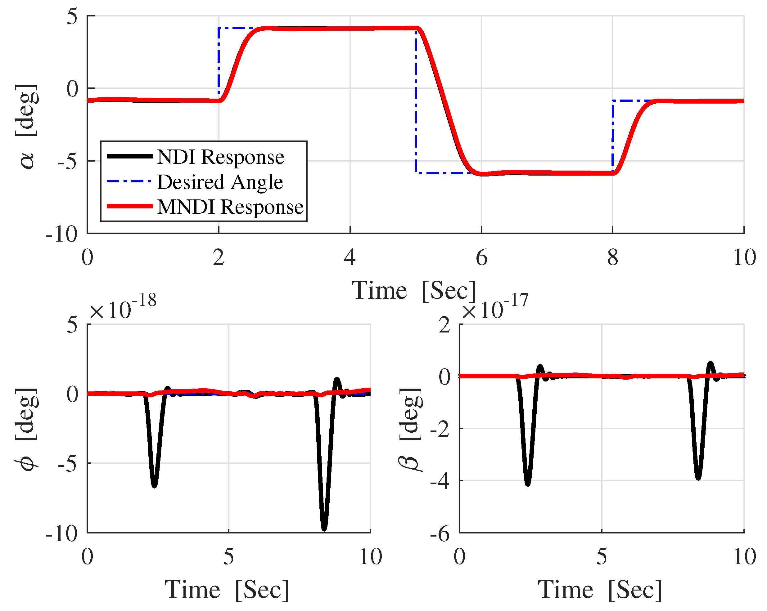
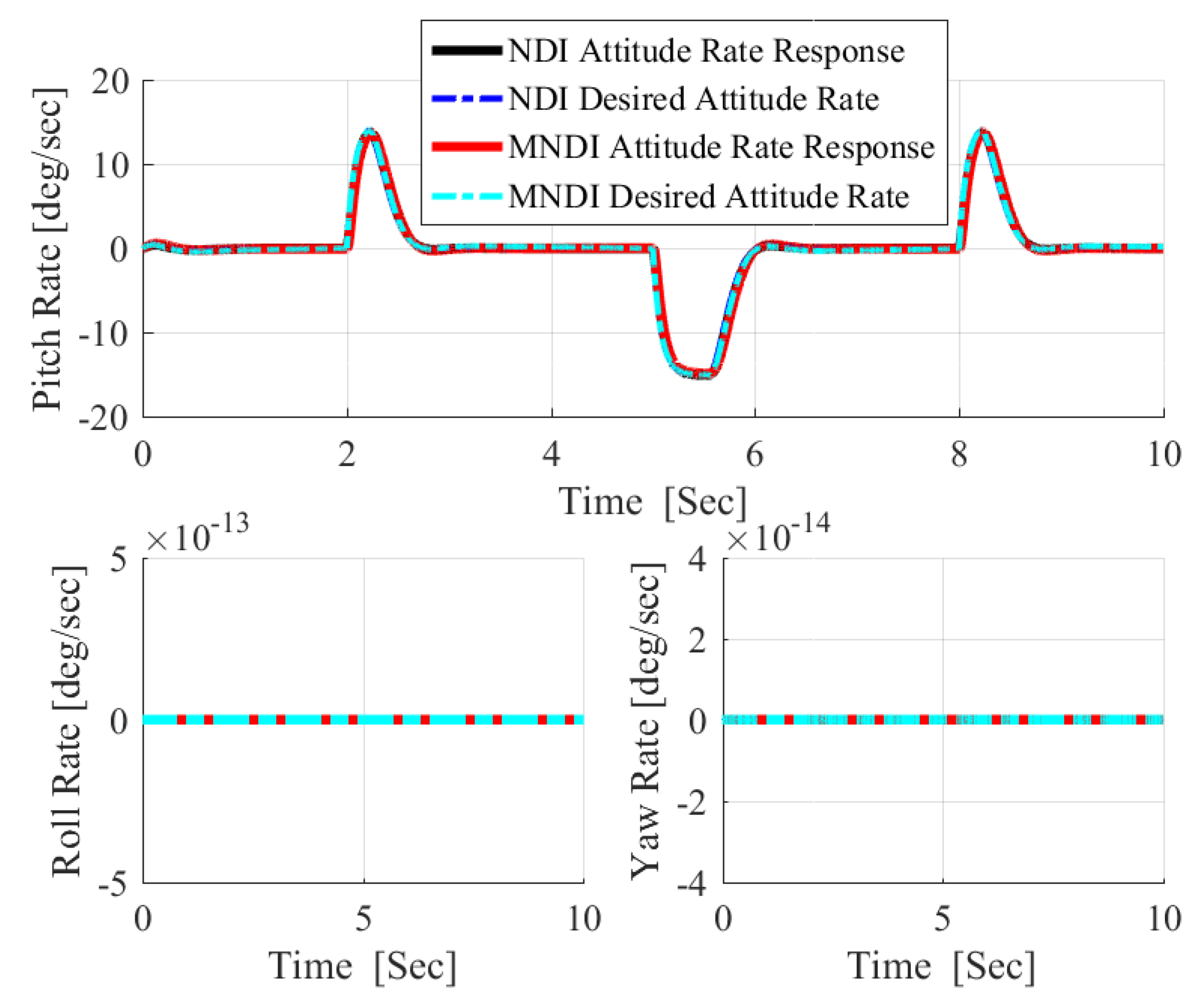
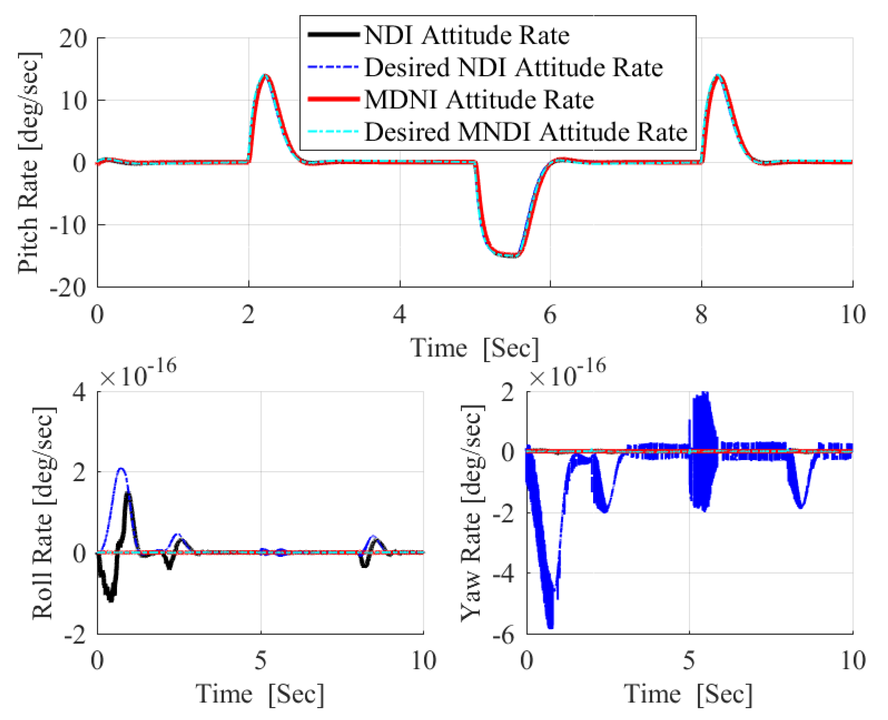
5.1. Robustness Analysis with NLDI and MNLDI

NLDI flight control technique is known to be a standard reference model for tracking commands because it amounts to canceling the nonlinearities in a nonlinear system so that the closed-loop dynamics is in a linear form. Consequently, it is prone to disturbances either internal such as model uncertainties or external such as wind disturbance. However, the asymptotic stability of the designed control laws given in Equations (7)–(9) for inner loop and Equations (20)–(22) for outer loop guarantee the robustness of NLDI against external wind disturbances. In contrast, the model-dependence flight controller failed to compensate for any small perturbation in the model parameter or unmodeled dynamics. On the other hand, MNLDI is capable of tracking the desired command despite the external wind disturbances, model uncertainties or unmodeled dynamic as it is a model independent flight controller. The conventional configuration of the fixed-wing Tiger-Trainer UAV is suffering from the coupling between the roll and yaw planes. Consequently, the lateral plane states are coupled while the longitudinal plane states are uncoupled. The simulation results focus on the ability of the designed flight control system to decrease the coupling between roll and yaw channels in addition to highlight the robustness of the designed flight controller against wind disturbances in addition to model uncertainties. Starting with pitch channel analysis of tracking performance and robustness analysis, the desired pitch angle command was compared with the actual UAV pitch angle in an ideal environment with neither wind disturbance nor model uncertainties. Moreover, the pitch angle response in severe wind disturbance conditions and high variation of the aerodynamic model was tested. Since the lateral plane coupling degrades the efficiency of the tracking performance and also increases the tendency to be sensible for disturbances, the decoupling capability of NLDI and MNLDI flight controllers was studied.

In Figure 6, a comparison between the performance of both flight controllers in response to pitch angle command with zero wind speed and accurate UAV model is illustrated. Pure feedback linearization was used successfully to address pitch angle tracking as NLDI cancels the unwanted nonlinear terms which force the control law to track the desired attitude with accepted performance. Not only NLDI meets the accepted tracking performance but also MNLDI is a good tracker, especially when it is optimally tuned. Generally, the coupling in the longitudinal plane is negligible in comparison with the lateral plane. However, MNLDI seems to eliminate the coupling between roll and yaw angles.

One of the important issues of tracking problem is the internal stability of the system under control. The most inner loop of the flight control system responds accurately to the outer attitude loop commands. Both NLDI and MNLDI are following the standard limitations of small fixed-wing UAV allowable rates [18]. In Figure 7, a comparison between the performance of angular rates inner loop tracking in response to pitch angle command without wind and accurate UAV model is illustrated.

Wind disturbance is a great challenge for the UAV flight control system, especially for small UAVs. Figure 8 confirms the robustness of the designed flight controller in both NLDI and MNLDI flight controller. Although the wind speed is very high compared with the Tiger-Trainer UAV, as it is $55\%$ of the UAV airspeed, the designed control law is able to withstand high constant high wind disturbance. The asymptotic stability of the designed control law guarantees best tracking performance with severs flight conditions. In Figure 9, a comparison between the performance of angular rates loop tracking in response to pitch angle command with high-speed wind is illustrated.

Uncertainties or unmodeled dynamics are the main challenges for the UAV flight control system, therefore a sinusoidal signal is added to $c_l,c_m,c_n$ aerodynamic roll, pitch, and yaw moment coefficients, respectively, given in [21] as uncertainty in aerodynamic model. In Figure 10, the perturbation signal amplitude is very high in comparison to the accurate model parameters.

The most important shortcoming associated with NLDI approach is the vulnerability to any uncertainties as it is a model-dependent control method, while MNLDI is robust against any model uncertainties as it is a model-independent flight control concept. Figure 11 shows the effect of the uncertain aerodynamic model given in Figure 10 in the performance of NLDI and MNLDI flight controller. NLDI is sensitive to the uncertainties; therefore, it is unable to track the desired references which confirms that the NLDI flight controller must be augmented with any other robust flight controller. In contrast, MNLDI is robust against model uncertainties; moreover, it still has absolute decoupling between roll and yaw angles. As a result, practically using MNLDI as a stand-alone flight control system is preferable. In Figure 12, the high amplitude angular rates performed by NLDI confirms the internal instability of using NLDI under model uncertainties. Meanwhile, MNLDI is still internally stable, as the angular rates required for achieving a sharp pitch maneuvers are within the allowable limits of angular rates.

In Figure 13, the difference between the desired attitude angle and the actual response of both flight controller confirms that MNLDI is more robust against than NLDI.

Secondly, the tracking performance and flight control robustness against the wind disturbances and unmodeled dynamics of the roll and yaw channels were analyzed. Due to the traditional shape of the Tiger UAV, there is a coupling between the lateral states, which decreases the accuracy of tracking the desired command with accepted performance which leads to instability. However, the robust flight controller must be able to handle all variations to keep tracking the desired command. Similar to the pitch channel, both NLDI and MNLDI are tracking the desired commands in accepted performances without any uncertainties or wind disturbances. Moreover, the designed law of control given in Equations (7)–(9) for inner loop and Equations (20)–(22) ensure of asymptotic error decaying regardless of the external wind disturbances. However, NLDI flight controller is unable to overcome the uncertainties introduced to the model as it is completely model dependent. Conversely, MNLDI is a robust flight control technique against wind disturbances and uncertainties.

The roll channel response is shown in Figure 14, which confirms the ability of MNLDI to overcome the model uncertainties and wind disturbances; meanwhile, NLDI is sensitive to the model uncertainties.

Figure 15 shows the need for the modification of NLDI to be able to overcome the model uncertainties; the high angular rates associated with the pure NLDI are beyond the allowable physical limitation of the Tiger-Trainer UAV, while MNLDI angular rates are within the limits. Figure 16 shows the effect of the wind disturbances on the desired command tracking for both NLDI and MNLDI. The error difference between the desired attitude angle and the actual response of both flight control technique proves that MNLDI is more robust against wind disturbances and model uncertainties that NLDI.

For more robustness analysis of the designed flight controller using MDI, a cross wind with speed 10 [m/s] and heading 90${}^{\circ }$ was applied. Figure 17 ensures of the asymptotic stability of the designed control law that guarantees best tracking performance with severs flight conditions.

In Figure 18, a comparison between the performance of angular rates tracking loop in response to roll angle command with high-speed cross wind is illustrated. MNLDI flight control technique is an internally stable system as the UAV attitude rates are still within the standard limit despite the cross wind.

In Figure 19, the difference between the desired and the actual attitude angle of both flight control technique confirms that MNLDI is more robust against wind disturbances and model uncertainties than NLDI.

The yaw channel response shown in Figure 20 is similar to the pitch and yaw channel’s response with a confirmation of the greater capability of MNLDI compared to pure NLDI in tracking reference commands with a strong wind disturbance and model uncertainties.

The associated angular rates in responding to yaw attitude command are shown in Figure 21, which show the need for modification on NLDI.

In Figure 22, the difference between the desired attitude angle and the actual response of both flight control technique confirms that MNLDI is more robust against wind disturbances and model uncertainties that NLDI.

To summarize the flight control segment, any small variations in the model will be accompanied with less tracking performance using NLDI flight controller. Therefore, NLDI flight controller is prone to parameter variations and misleads the desired command. In contrast, MNLDI is robust against model uncertainties; consequently, it is guaranteed as a stand-alone flight control system.

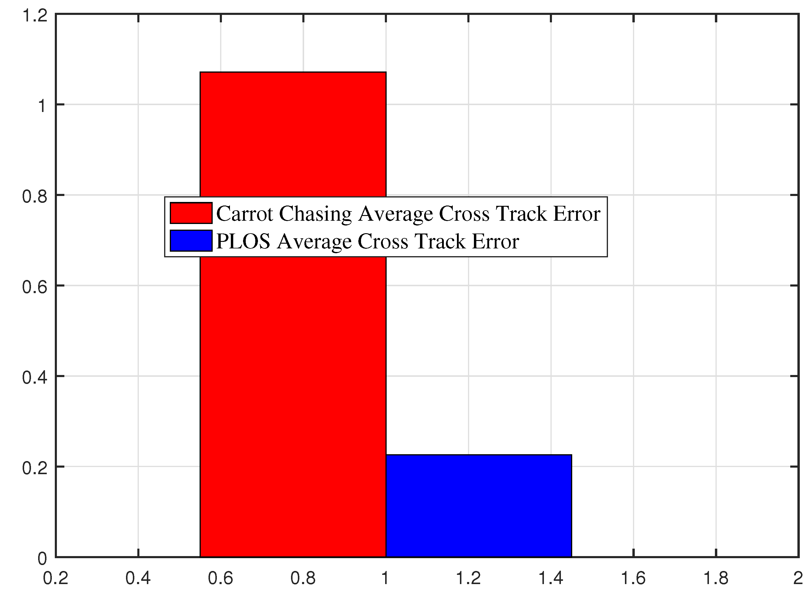
5.2. Evaluation of Two UAV Path Following Algorithms

The following sharp maneuvers guarantees the ability of the flight control system to achieve different missions. This section highlights the ability of carrot chasing and PLOS path following methods to track the predetermined path. As aforementioned, MNLDI is accepted in tracking performance while guaranteeing robustness against external disturbances in addition to it is non-sensitive to the uncertainties. Therefore, MNLDI flight control system was used as the inner control loop for the outermost guidance loop.

For carrot chasing algorithm, the optimal weighting values for the control gain k and the VTP distance $\delta$ were chosen on the trial and error basis. The selection of VTP distance $\delta$ controls the performance of the UAV following the desired path. If $\delta$ is small, the UAV oscillates around the desired path, thus increasing the cross-track error distance, which prevents the UAV from riding the path early. By increasing the value of $\delta$, the UAV quickly rides the desired path. The maximum value of $\delta$ is constrained by the value of cross-track error. Consequently, $\delta$ is increased until a certain point, beyond which the cross-track error increases again and UAV fluctuates around the desired path.

For PLOS path following guidance algorithm, the advantages of the combination of two guidance laws are exploited; one keeps the LOS angle while the other minimizes the cross-track error distance. If the pursuit guidance gain $k_1$ in Equation (2) is a small positive number, then the UAV oscillates around the desired path.

The proposed sequence of the desired waypoints highlights the ability of the UAV to follow abrupt maneuvers with different LOS angles starting from acute angles to obtuse angles $\theta =$ 10:180 [deg] passing through sharp change square LOS angle $\theta =$ 90 [deg] excluding the transient errors from the turns. The critical practical problem is associated with the flight control system with external wind disturbances, however using the geometric path following algorithm with the robust MNLDI guarantees a stable platform that meets the desired performance criteria. In the following analysis, the effect of constant west wind with a speed half the Tiger-Trainer UAV cruise speed was introduced. In each scenario, just touching a circumferential circle around the desired waypoint with radius r = 130 [m] was required.

In Figure 23, a comparison between carrot chasing and PLOS guidance method for following a predetermined path is illustrated. The cross-track error and LOS angles are compensated by generating bank angle commands based on the position of the UAV to the desired waypoint. After touching the circle centered by the desired waypoint location, the algorithm switches to the next desired waypoint.

Figure 24 illustrates the robustness of the proposed flight control model against wind disturbance. With constant altitude, the pitch channel control law regulates the desired trim altitude for the Tiger-Trainer UAV $h=200\left[\mathrm{m}\right]$. Meanwhile, the roll channel control law responds to the desired bank angle to achieve required turning. The altitude hold control loop keeps the altitude constant despite the sharp change of the bank angles to turn in responding to different sharp maneuvers, as shown in Figure 25. Similarly, the velocity maintains the UAV on the desired position along the given path, as shown in Figure 26.

The cross track error shown in Figure 27 confirms that the PLOS path following guidance law is more robust against wind disturbances than the carrot chasing path following guidance law. Since PLOS is a combination of two guidance laws, controlling the cross-track error is a main part of the generated guidance law that leads to a rapid decreasing of the error. The mean of the cross-track error for both methods is illustrated in Figure 28, which indicates that PLOS path following guidance method proves to be more practical than carrot chasing path following guidance law.

6. Conclusions

In this study, a detailed analysis of two autonomous path-following guidance algorithms was performed with NLDI and MNLDI flight control systems using a small UAV model, which is a nonlinear 6-DOF rigid body model. NLDI is a powerful flight controller for the accurate model by designing asymptotic stable control law. However, the accurate model is unavailable, therefore a modification was required to increase the flight control robustness against wind disturbances and model uncertainties. The simulation results demonstrate the effectiveness of the designed stable flight control law using NLDI and highlight its limitation against inaccurate model parameters. However, MNLDI control law is proved to be robust against internal and external disturbances because the designed control law is model-independent. The idea of path following based on carrot chasing and PLOS has been extended to constant altitude path following. It has been shown using MNLDI controlling heading rate based on tracking a VTP. The effectiveness of the described following algorithms have been illustrated; the UAV followed the desired paths with an asymptotically decaying error. The two paths following algorithms proved effective in following sharp straight-line segments maneuvers. From the analysis, one can easily select the convenient path following algorithm and tune it appropriately. The flight simulation results confirm that PLOS path following algorithm more accurately followed the path than carrot chasing which is prone to wind disturbance.

References

- Nelson, D.R.; Barber, D.B.; McLain, T.W.; Beard, R.W. Vector Field Path Following for Miniature Air Vehicles. IEEE Trans. Robot. 2007, 23, 519–529. [Google Scholar] [CrossRef] [Green Version]
- Patel, M.; Jernigan, S.; Richardson, R.; Ferguson, S.; Buckner, G. Autonomous Robotics for Identification and Management of Invasive Aquatic Plant Species. Appl. Sci. 2019, 9, 2410. [Google Scholar] [CrossRef]
- Kaminer, I.; Pascoal, A.; Hallberg, E.; Silvestre, C. Trajectory tracking for autonomous vehicles: An integrated approach to guidance and control. J. Guid. Control. Dyn. A Publ. Am. Inst. Aeronaut. Astronaut. Devoted Technol. Dyn. Control 1998, 21, 29–38. [Google Scholar] [CrossRef]
- Sujit, P.B.; Saripalli, S.; Sousa, J.B. Unmanned Aerial Vehicle Path Following: A Survey and Analysis of Algorithms for Fixed-Wing Unmanned Aerial Vehicless. IEEE Control Syst. 2014, 34, 42–59. [Google Scholar]
- Qiu, B.; Wang, G.; Fan, Y.; Mu, D.; Sun, X. Adaptive Sliding Mode Trajectory Tracking Control for Unmanned Surface Vehicle with Modeling Uncertainties and Input Saturation. Appl. Sci. 2019, 9, 1240. [Google Scholar] [CrossRef]
- Enomoto, K.; Yamasaki, T.; Takano, H.; Baba, Y. Guidance and Control System Design for Chase UAV. AIAA Guid. Navig. Control Conf. Exhib. 2013, 976–984. [Google Scholar] [CrossRef]
- Ambrosino, G.; Ariola, M.; Ciniglio, U.; Corraro, F.; De Lellis, E.; Pironti, A. Path Generation and Tracking in 3-D for UAVs. IEEE Trans. Control Syst. Technol. 2009, 17, 980–988. [Google Scholar] [CrossRef]
- Park, S.; Deyst, J.; How, J.P. Performance and lyapunov stability of a nonlinear path-following guidance method. IEEE J. Guid. Control Dyn. 2007, 30, 1718–1728. [Google Scholar] [CrossRef]
- Sujit, P.B.; Saripalli, S.; Sousa, J.B. An evaluation of UAV path following algorithms. In Proceedings of the 2013 European Control Conference, Zurich, Switzerland, 17–19 July 2013; pp. 3332–3337. [Google Scholar]
- Mori, K.; Takahashi, M. Minimum-Time Attitude Maneuver and Robust Attitude Control of Small Satellite Mounted with Data Relay Communication Antenna. Appl. Sci. 2019, 9, 1001. [Google Scholar] [CrossRef]
- Sun, M.; Zhu, R.; Yang, X. UAV Path Generation, Path Following and Gimbal Control. In Proceedings of the 2008 IEEE International Conference on Networking, Sensing and Control, Sanya, China, 6–8 April 2008; pp. 870–873. [Google Scholar]
- Rhee, I.; Park, S.; Ryoo, C.-K. A tight path following algorithm of an UAS based on PID control. In Proceedings of the SICE Annual Conference 2010, Taipei, Taiwan, 18–21 August 2010. [Google Scholar]
- Cunha, R.; Silvestre, C.; Pascoal, A. A path following controller for model-scale helicopters. In Proceedings of the European Control Conference (ECC), Cambridge, UK, 1–4 September 2003; pp. 2248–2253. [Google Scholar]
- Ratnoo, A.; Sujit, P.B.; Kothari, M. Adaptive Optimal Path Following for High Wind Flights. IFAC Proc. Vol. 2011, 44, 12985–12990. [Google Scholar] [CrossRef] [Green Version]
- Niu, H.; Lu, Y.; Savvaris, A.; Tsourdos, A. Efficient path following algorithm for unmanned surface vehicle. Oceans 2016. [Google Scholar] [CrossRef]
- Kothari, M.; Postlethwaite, I. A Probabilistically Robust Path Planning Algorithm for UAVs Using Rapidly-Exploring Random Trees. J. Intell. Robot. Syst. 2013, 71, 231–253. [Google Scholar] [CrossRef]
- Slotine, J.-J.E.; Li, W.P. Applied Nonlinear Control; United States Edition; Prentice Hall: Englewood Cliffs, NJ, USA, 1991. [Google Scholar]
- Beard, R.W.; McLain, T.W. Small Unmanned Aircraft: Theory and Practice; Princeton University Press: Princeton, NJ, USA, 2012. [Google Scholar]
- Tran, D.-T.; Truong, H.-V.-A.; Ahn, K.K. Adaptive Backstepping Sliding Mode Control Based RBFNN for a Hydraulic Manipulator Including Actuator Dynamics. Appl. Sci. 2019, 6, 1265. [Google Scholar] [CrossRef]
- Snell, S.A.; Nns, D.F.; Arrard, W.L. Nonlinear inversion flight control for a supermaneuverable aircraft. J. Guid. Control. Dyn. 1992, 15, 976–984. [Google Scholar] [CrossRef]
- Kamal, A.M.; Bayoumy, A.M.; Elshabka, A.M. Modeling and flight simulation of unmanned aerial vehicle enhanced with fine tuning. Aerosp. Sci. Technol. 2016, 51, 106–117. [Google Scholar] [CrossRef]
© 2019 by the authors. Licensee MDPI, Basel, Switzerland. This article is an open access article distributed under the terms and conditions of the Creative Commons Attribution (CC BY) license (http://creativecommons.org/licenses/by/4.0/).
Share and Cite
Safwat, E.; Zhang, W.; Mohsen, A.; Kassem, M. Design and Analysis of a Robust UAV Flight Guidance and Control System Based on a Modified Nonlinear Dynamic Inversion. Appl. Sci. 2019, 9, 3600. https://doi.org/10.3390/app9173600
Safwat E, Zhang W, Mohsen A, Kassem M. Design and Analysis of a Robust UAV Flight Guidance and Control System Based on a Modified Nonlinear Dynamic Inversion. Applied Sciences. 2019; 9(17):3600. https://doi.org/10.3390/app9173600
Chicago/Turabian StyleSafwat, Ehab, Weiguo Zhang, Ahmed Mohsen, and Mohamed Kassem. 2019. "Design and Analysis of a Robust UAV Flight Guidance and Control System Based on a Modified Nonlinear Dynamic Inversion" Applied Sciences 9, no. 17: 3600. https://doi.org/10.3390/app9173600