Classifying Power Quality Disturbances Based on Phase Space Reconstruction and a Convolutional Neural Network

Abstract

This paper presents a hybrid approach combining phase space reconstruction (PSR) with a convolutional neural network (CNN) for power quality disturbance (PQD) classification. Firstly, a PSR technique is developed to transform a 1D voltage disturbance signal into a 2D image file. Then, a CNN model is developed for the image classification. The feature maps are extracted automatically from the image file and different patterns are derived from variables in CNN. A set of synthetic signals, as well as operational measurements, are used to validate the proposed method. Moreover, the test results are also compared with existing methods, including empirical mode decomposition (EMD) with balanced neural tree (BNT), S-transform (ST) with neural network (NN) and decision tree (DT), hybrid ST with DT, adaptive linear neuron (ADALINE) with feedforward neural network (FFNN), and variational mode decomposition (VMD) with deep stochastic configuration network (DSCN). Based on deep learning algorithms, the proposed method is capable of providing more accurate results without any human intervention for PQDs. It also enables the planning of PQ remedy actions.

1. Introduction

In the last three decades, the penetration of renewable energy into the power grid network has increased. This gives rise to power quality (PQ) issues. The same is true with increasing uptake of wind turbines, solar energy, and energy storage systems [1,2]. These disturbances greatly affect the safe and economical operations of smart grid networks and decrease the lifetime and power conversion efficiency and reliability of grid-connected renewable energy systems. Therefore, PQ analysis, including disturbance recognition and classification, is a crucial task to provide adequate information for further remedial actions. For instance, faulty power equipment can be discovered so that predictive maintenance can be scheduled in time. If power quality disturbance signals are detected, the control strategy of power converters can also be optimized to avoid catastrophic failures [3,4].

In essence, PQ refers to multifarious electromagnetic phenomena that cause deviations in voltage and current from their ideal waveforms, which are known as PQ disturbances (PQDs). The presence of PQDs can be divided into sags, swells, interruptions, oscillations, flickers, harmonics, notches, spikes, and their combinations, as per international standards such as EN 50160 [5], IEC 61000 [6], and IEEE-1159 [7]. The conventional methods of PQD recognition and classification contain two steps: feature extraction and classification. The feature extraction methods are mostly based on signal processing techniques, such as Fourier transform (FT) [8], short time Fourier transform (STFT) [9,10], wavelet transform (WT) [11,12,13], S-transform (ST) [14,15], empirical mode decomposition (EMD) [16,17,18], independent component analysis (ICA) [19], and variational mode decomposition (VMD) [20,21,22]. These methods are used to extract features from different types of PQDs. Then, the disturbance classification is conducted by a specific rule according to the features. In the literature, typical methods are decision tree (DT) [23,24], artificial neural network (ANN) [25], probabilistic neural network (PNN) [26,27], and support vector machine (SVM) [28,29]. In [3], a knowledge-based waveform analysis method is used to inform utilities of the condition and health of individual components in the power system. It is focused on component issues influenced by power quality problems. A generic waveform abnormality detection method is adopted in [4]. In this paper, a Kullback–Leibler divergence (KLD) is developed as a threshold to detect the abnormality of the grid voltage and current. It can identify abnormal conditions precisely, but cannot give the type of the PQD. Although the existing methods are effective, they have some limitations: (1) They make use of synthetic PQD signals as per international standards, which do not represent the actual signals faithfully; (2) Different types and quantities of the features have a great influence on the classification results. For PQD classification, it is difficult to know what features should be extracted. In current research, the process of feature extraction relies heavily on various handcrafted features with different number and type, for example, relative mode energy ratio (RMER), mode’s center frequency, number of zero-crossings, and instantaneous amplitude (IA) are used in [21]; mean, variance, and kurtosis are used in [22]. Taking inappropriate features decreases the accuracy of the classifier; (3) These methods all belong to the shallow model in nature. It has been validated that deep learning models are much more powerful than the shallow models due to their deep layer topology and big data support [30,31]. In this paper, it is essential to develop new deep learning-based techniques for PQDs classification in order to extract features automatically, and simultaneously analyze all the nonlinear, nonstationary synthetic and operational signals.

In deep learning technologies, convolutional neural networks (CNNs) have become an emerging and popular technique. They are applied to a wide range of tasks related to signal, image, and information processing in the artificial intelligence (AI) domain [30]. Deep learning algorithms have the powerful capability of learning optimal features from raw input data automatically through using multiple levels of abstraction and representation of the signal and image data. Furthermore, big data and availability of large-scale computing power by using graphical processing units (GPUs) provide great support for deep learning techniques. In the literature, several methodologies based on deep learning are presented to identify the types of PQDs. The estimation of voltage sag in sparsely monitored power systems by using the CNN model is adopted in [32]. In [33], the CNN combined with a long short-term memory (LSTM) method is used for PQDs classification. The PQDs are estimated based on a deep belief network (DBF) in [34]. Although these methods obtain good performance for PQDs analysis, some limitations can be identified.

This paper proposes a novel method combining phase space reconstruction (PSR) with CNN for PQD detection and classification. The PSR method is firstly used to transform 1D raw data of PQD into a 2D image file. Then, a CNN model is developed for the image classification. The novelty of this proposed method is that the traditional PQDs classification problem has been mapped into an image classification issue, which is the expertise of CNNs. The performance of the proposed method is tested and validated by ten types of synthetic PQDs as well as operational signals from the IEEE Working Group on Power Quality Data Analytics.

This paper is organized as follows: Section 2 presents the proposed algorithms based on the PSR and CNN models. Section 3 introduces the implementation of the PSR-CNN method for PQDs classification. Section 4 presents the discussion and classification results using different types of synthetic cases and operational signals. Finally, concluding remarks are made in Section 5.

2. Methodologies

This section provides an overview of the related algorithms used for PQD classification in the proposed method. The principle and realization of the theories are illustrated in detail.

2.1. The Principles of Phase Space Reconstruction

The basic concept of phase space reconstruction is to treat the value of a specific variable at a certain moment and those values after $\tau ,$ $2\tau ,$..., $\left(m-1\right)\tau$ time intervals as coordinates of a special point in $m$-dimension phase space [35]. A graphical representation of a nonlinear system can be obtained through describing a sequence of data points in the above phase space. An $m$-dimensional phase space can be constructed from a single time series variable $x_1, x_2, \dots , x_N$ by introducing the embedding dimension parameter $m$ and delay time $\tau$:

$$X_i={[x_i, x_{i+\tau }, \dots , x_{i+\left(m-1\right)\tau }]}^T$$

(1)

where $i=1, 2, \dots , L, L=N-\left(m-1\right)\tau$, $N$ is the number of sample points. Then, a phase space matrix can be obtained, which represents the coordinates of the signal trajectory:

$$\mathrm{X}=\left[\begin{array}{c}{X}_1\\ X_2\\ ⋮\\ X_L\end{array}\right]={\left[\begin{array}{c}{x}_1, x_{1+\tau }, \dots , x_{1+\left(m-1\right)\tau }\\ x_2, x_{2+\tau }, \dots , x_{2+\left(m-1\right)\tau }\\ ⋮\\ x_L, x_{L+\tau }, \dots , x_{L+\left(m-1\right)\tau }\end{array}\right]}^T$$

(2)

In essence, the phase space reconstruction trajectory is the strange attractor of a time series data in a chaotic system [36], e.g., electroencephalogram, short time power load, and stock exchange. In this paper, the disturbance components carried by periodical voltage signals are considered and a $x\left(t\right)-x\left(t+\tau \right)$ phase space is constructed to describe the signal trajectory. Hence, the 1D time series data of PQDs are mapped into 2D images, which serve as the input data to the CNN model for PQD classification. By comparing the traditional time–frequency-based feature extraction methods, the PQDs can be identified from a graphic perspective in the time domain, which overcomes the spectrum aliasing problem in the time–frequency transforming process.

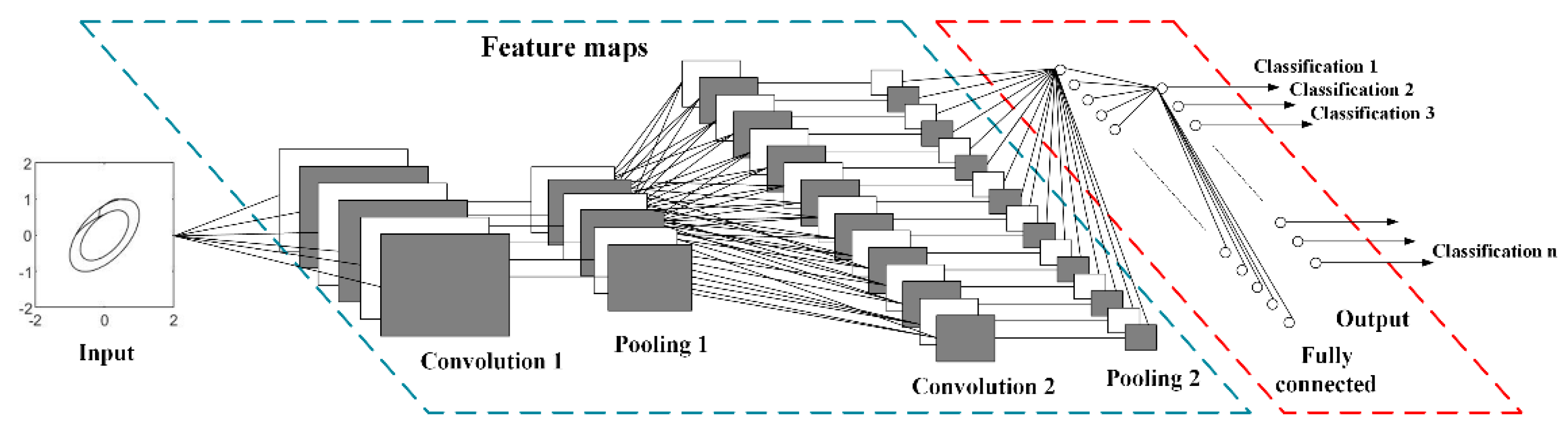
2.2. The Theory of the Convolutional Neural Network

The CNN is a biologically inspired feedforward artificial neural network (ANN) that presents a simple model for the mammalian visual cortex. It has been widely used in the visual field, such as image recognition [37,38] and video classification [39]. A fundamental framework of the CNN model is illustrated in Figure 1. Typically, CNN architectures consist of an input layer, convolution layers, pooling layers, fully connected layers, and an output layer. The convolution layer uses the mathematical 2D convolution operation to transform low-level local features into high-level global features. It consists of multiple filters ${\mathit{W}}^{\mathit{k}}$, each giving rise to an output feature map. This map $h^k$ corresponds to the weight matrix ${\mathit{W}}^{\mathit{k}}$ of the $k$th filter and can be obtained by:

$$h_{ij}^k=f{\left({\mathit{W}}^{\mathit{k}}\ast x\right)}_{ij}+b^k$$

(3)

where the sign $\ast$ is the mathematical 2D convolution operation, $x$ is the input data of this layer, $b$ is a bias term, and $f(·)$ is a nonlinear activation function. The weight-sharing technique adopted between neurons in different layers helps the process of feed forward and backpropagation (BP) [40] to reduce the number of parameters under consideration. Through the convolution layer, the hidden invariant features in the data are extracted automatically and effectively. The pooling layer implements nonlinear downsampling after the convolution layer through a max-pooling (or average-pooling) method. The output of the convolution layer is divided into a set of nonoverlapping rectangles, outputting the maximum (or average) of each subregion. The aim of this layer is to reduce the spatial size of the representation progressively, decrease the number of parameters, and avoid overfitting. A fully connected layer combines all the feature maps to produce the final classification vector to the output layer.

3. The Proposed Algorithm of PQDs Detection and Classification Based on PSR and CNN

In this section, the mathematical models of the PQD signals are firstly presented; then, the framework and training process of the proposed method are demonstrated.

3.1. PQ Disturbance Model

To illustrate the use of the PSR-CNN method for PQDs classification, ten types of single and mixed voltage disturbance signals have been synthesized in MATLAB according to the IEEE-1159. The labels and numerical models are presented in

Table 1. Results of variational mode decomposition (VMD) for power quality disturbances (PQDs) with harmonics and interharmonics extraction.

PQ Disturbance	Label	Numerical Model	Parameters
Sag	Sag	$v\left(t\right)=\left(1-\alpha \left(u\left(t-t_1\right)-u\left(t-t_2\right)\right)\right)sin\omega t$	$0.1\le \alpha \le 0.9,T\le t_2-t_1\le 9T$
Swell	Swell	$v\left(t\right)=\left(1+\alpha \left(u\left(t-t_1\right)-u\left(t-t_2\right)\right)\right)sin\omega t$	$0.1\le \alpha \le 0.8,T\le t_2-t_1\le 9T$
Interruption	Inter	$v\left(t\right)=\left(1-\alpha \left(u\left(t-t_1\right)-u\left(t-t_2\right)\right)\right)sin\omega t$	$0.9\le \alpha \le 1,T\le t_2-t_1\le 9T$
Flicker	Flicker	$v\left(t\right)=\left(1+{\alpha }_f\sin \left(\beta \omega t\right)\right)sin\omega t$	$0.1\le {\alpha }_f\le 0.2,5\le \beta \le 20Hz$
Harmonic	Har	$v\left(t\right)={\alpha }_{1}sin\omega t+{\alpha }_{3}sin3\omega t+{\alpha }_{5}sin5\omega t$	$0.05\le {\alpha }_3,{\alpha }_5\le 0.15$, ${{\displaystyle \sum }}^{ }{\alpha }_i{}^2=1$
Oscillatory Transient	Osc	$v\left(t\right)=sin\omega t+\alpha e^{-\frac{\left(t-t_1\right)}{{\tau }_0}}sin{\omega }_n\left(t-t_1\right)\times$$\left\{u\left(t_2\right)-u\left(t_1\right)\right\}$	$0.1\le \alpha \le 0.8,$ $0.5T\le t_2-t_1\le 3T,$ $8ms\le {\tau }_0\le 40ms,$ $300\le f_n\le 900Hz$
Spike	Spike	$v\left(t\right)=sin\omega t+sign\left(sin\omega t\right)\times$$\left[{\displaystyle \sum }_{n=0}^{9}K\times \left\{u\left(t-\left(t_1+0.02n\right)\right)-u\left(t-\left(t_2+0.02n\right)\right)\right\}\right]$	$0.1\le K\le 0.4,0\le t_1,t_2\le 0.5T$ $0.01T\le t_2-t_1\le 0.05T$
Sag & Harmonic	Sag & Har	$v\left(t\right)=\left(1-\alpha \left(u\left(t-t_1\right)-u\left(t-t_2\right)\right)\right)\times$$\left({\alpha }_{1}sin\omega t+{\alpha }_{3}sin3\omega t+{\alpha }_{5}sin5\omega t\right)$	$0.1\le \alpha \le 0.9,T\le t_2-t_1\le 9T$ $0.05\le {\alpha }_3,{\alpha }_5\le 0.15$, ${{\displaystyle \sum }}^{ }{\alpha }_i{}^2=1$
Interruption & Harmonic	Inter & Har	$v\left(t\right)=\left(1-\alpha \left(u\left(t-t_1\right)-u\left(t-t_2\right)\right)\right)\times$$\left({\alpha }_{1}sin\omega t+{\alpha }_{3}sin3\omega t+{\alpha }_{5}sin5\omega t\right)$	$0.9\le \alpha \le 1,T\le t_2-t_1\le 9T$ $0.05\le {\alpha }_3,{\alpha }_5\le 0.15$, ${{\displaystyle \sum }}^{ }{\alpha }_i{}^2=1$
Swell & Harmonic	Swell & Har	$v\left(t\right)=\left(1+\alpha \left(u\left(t-t_1\right)-u\left(t-t_2\right)\right)\right)\times$$\left({\alpha }_{1}sin\omega t+{\alpha }_{3}sin3\omega t+{\alpha }_{5}sin5\omega t\right)$	$0.1\le \alpha \le 0.8,T\le t_2-t_1\le 9T$ $0.05\le {\alpha }_3,{\alpha }_5\le 0.15$, ${{\displaystyle \sum }}^{ }{\alpha }_i{}^2=1$

. The amplitude of the simulated signals are normalized to 1 p.u. and the fundamental frequency is 50 Hz. These PQDs are all simulated over the defined parameter range as shown in Table 1.

Next, a 2D image is generated by the PSR method. The delay time $\tau$ is an important parameter of the PSR method. A good choice of $\tau$ facilitates the performance analysis. If the value is low, the adjacent successive elements $x_{i+\tau }$ and $x_{i+2\tau }$ of the vectors are strongly correlated; if it is high, the adjacent elements are almost independent. The effect of $\tau$ for the attractor construction is the expansion degree of the diagonal in the phase plane. The trajectory can be expanded at the utmost around the diagonal, which is a function of τ. To choose an appropriate delay time $\tau$, a mutual information function of the system $\left[s, q\right]=\left[x\left(t\right), x\left(t+\tau \right)\right]$ [35] is used in this paper:

$$I\left(S, Q\right)={\displaystyle \sum }_i{\displaystyle \sum }_j{P}_{sq}\left(s_i, q_j\right)\log [\frac{P_{sq}\left(s_i, q_j\right)}{P_s\left(s_i\right)P_q\left(q_j\right)}]$$

(4)

where $P_s\left(s_i\right)$, $P_q\left(q_j\right)$ and $P_{sq}\left(s_i, q_j\right)$ are the probabilities and the joint probabilities of the events $s_i$, $q_j$ [39], respectively. A delay time $\tau$ is determined by dropping the $I\left(S, Q\right)$ value to a sufficient small value $\frac{1}{e}$ [35].

Specifically, the sample frequency $f_s$ is 6.4 kHz, the number of sample points in one cycle is 200, and there are 10 cycles in every synthetic signal. In addition, the dimension parameter $m$ of the PSR method is 2 and the delay time $\tau$ is 20 according to (4). Then, the 2D images of the PQD signals are transformed by the PSR method and illustrated in Figure 2. The size of every image is 200 × 200 pixels.

3.2. The Proposed Method

The main framework of the proposed method is illustrated in Figure 3. A CNN model composed of three convolution layers, two pooling layers, a fully connecting layer, and an output layer is established. The number of the convolution kernels in different layers are 32, 48, and 64, respectively.

Herein, the image features are extracted by the convolution operator to preserve the spatial relationship between pixels in the image matrix. A feature map is produced by a kernel based on the input image. In this paper, three kinds of convolution kernel with two different size (5 × 5 and 3 × 3) are used. For the sake of simplicity, a 5 × 5 convolution kernel is taken for example and the convolution operation is implemented by:

$$c_{ij}^k={{\displaystyle \sum }}_{m=0}^4{{\displaystyle \sum }}_{n=0}^4{w}_{m, n}{x}_{i+m,j+n}+b^k$$

(5)

where $w$ is the weight of the kernel, $x$ is the input data of this layer, $b$ is a bias term, $c$ is the result of convolution operation, $k$ is the number of kernels, and $i, j$ and $m, n$ are the location labels of the original image and convolution kernel matrices, respectively.

The implementation of the convolution operator is illustrated in Figure 4. A kernel slides over the input image by using (5) to produce a feature map and the stride size of the sliding is 1. To guarantee the process of feature extraction, the zero padding method is used to preserve the information of the input volume. The convolution of another kernel over the same image gives a different feature map. Actually, the convolution operation captures the local dependencies in the input image and different feature maps are generated by different kernels. An additional operation, called activation, is performed after every convolution layer. The purpose of this process is to introduce nonlinearity in the CNN model for better learning the nonlinear PQDs data. Herein, the rectified linear unit (ReLU) activation function is adopted to fulfill the nonlinear activation requirements due to its advantages of faster training speed and gradient vanishing problem alleviation. The function of ReLU is illustrated as:

$$f\left(x\right)=max\left(0,x\right)$$

(6)

Commonly, a pooling layer is added after the ReLU function to continuously reduce the dimensionality and number of parameters of the network. It shortens the time for the training computation and effectively controls overfitting. The average pooling method instead of max pooling is used because it retains the true feature of the sparse PQD image matrix. Finally, the fully connected layer, which is a traditional multilayer perceptron, uses a softmax function to estimate the classification vector to the output layer.

3.3. The Training of the Model

A training process is needed to improve the effectiveness of the model. The overall training process is carried out by six steps:

Step 1: Initialize all the parameters of the kernels with random values.

Step 2: Divide the original images into training and testing sets. The model goes through the forward propagation step (convolution, ReLU, pooling, and fully connected layers) and determines the output probabilities for each class with a training image.

Step 3: A cross entropy function is used as a cost function to calculate the error at the output layer:

$$e_i=-{{\displaystyle \sum }}_{i=1}^n\widehat{y_i}ln{y}_i$$

(7)

where $e_i$ is the error of the $i$th type of PQDs, $y_i$ is the target probability, and $\widehat{y_i}$ is the output probability.

Step 4: Calculate the gradients of the error with respect to all weights and parameters in the model by using the BP technique. Then, the gradient descent is used to update all the parameter values of the kernels to minimize the output error.

Step 5: Repeat Steps 2–4 with all images in the training set until the error is within the preset value.

Step 6: After the training process, the testing set is used to validate the accuracy of the model.

4. Results and Discussion

The effectiveness of the proposed method is verified in this paper for PQD detection and classification. The test data are generated through both synthetic and operational signals in a smart grid system.

4.1. Synthetic Signals

As illustrated in Section 3, ten voltage disturbances were established in MATLAB. For each disturbance, there are 400 sample signals, where 320 are for training and 80 are for validation.

A CNN model is established for the PQD 2D image training. In total, ten epochs are adopted in the training progress to obtain optimal parameters of the model. The hardware for the model training is based on an Intel (R) Core (TM) i7-6700HQ CPU @ 2.6GHz, 16 GB RAM and NVIDIA GeForce GTX 970M GPU with 192-bit 4 GB GDDR5 memory. The training process lasts 111 min and 52 s. The training progress and the confusion matrices of training and validation results are shown in Figure 5 and Figure 6, respectively.

In Figure 5, the high classification rate can be obtained only after five epochs and the loss of the cost function was almost zero. In Figure 6a, the classification rate in the training confusion matrix was 100% for both single and mixed synthetic disturbances. While 80 events were used for validation, the total classification rate was 99.8%, as shown in Figure 6b. The results demonstrate that the proposed method based on the PSR and CNN can achieve an excellent classification rate for PQDs. Additionally, the accuracy comparison of the proposed PQ assessment framework with other methods was illustrated in

Table 2. Comparison of the proposed PQDs with other methods.

Method	Feature Extraction (Handcrafted/Automatically)	No. PQDs	Accuracy. (%)	Ref.
EMD+Balanced Neural Tree	Handcrafted	8	97.9	[41]
ST+NN+DT	Handcrafted	13	99.9	[25]
Hybrid ST+DT	Handcrafted	11	94.36	[42]
ADALINE+FNN	Handcrafted	12	90.58	[43]
VMD+DeepSCN	Handcrafted	7	99.4	[22]
PSR+CNN	Automatically	10	99.8	Proposed method

with five methods, including EMD with balanced neural tree [41], ST with NN and DT [25], Hybrid ST with DT [42], ADALINE with FNN [43], and VMD with DSCN [22]. In Table 2, the proposed method is shown to be as good as the current best methods in terms of accuracy, as the 99.67–99.90% accuracy is well within the measurement uncertainty. The novelty of this work lies in the deep learning-based classification method and automatic feature extraction, while the existing methods are handcrafted. The features extracted by the convolution layers are shown in Figure 7. It can be seen that the feature maps are different even in one layer. For the different convolution layers, the extracted features are more specific when going to deep levels. Moreover, the weights of a convolution kernel are different too, leading to different pattern calculations for different variables. The evaluation results show that the proposed framework has comparatively better performance than the existing methods.

4.2. Real-World Signals

Following the synthetic signals, four types of operational voltage disturbance signals were measured and provided online at the IEEE Working Group on Power Quality Data Analytics [44], including sag, swell, sag and harmonic, and swell and harmonic. For each disturbance, there are 20 sample signals, of which the fundamental frequency is 60 Hz and which are sampled at 7.6 kHz. The number of sample points in one cycle is 128 and there are eight cycles in every signal. Several operational signals are needed to participate in the training process to fine-tune the parameters of the existing mode. To choose an optimal number of operational signals, a different number of synthetic signals of each disturbance from the training data used in the previous section were randomly replaced by the real-world signals. Then, the new training data were used to fine-tune the CNN model. Finally, the fine-tuned model was validated by using the operational data. The results are shown in Figure 8. It can be seen that a low classification rate (20%) is obtained without the fine-tuning process. Then, the classification rate improves (97.5%) with the five real-world signals used. The classification rate reaches the highest point (98.8%) when the number of operational signals is seven. Hence, in order to improve the performance of the classification of operational voltage disturbances, seven synthetic signals of each disturbance from the training data were randomly replaced with real-world signals. The validation confusion matrix is shown in Figure 9. The features extracted by the convolution layers are presented in Figure 10. In total, 20 events for each disturbance were used for validation and the total classification rate was 98.8%, as shown in Figure 9. It is observed that the proposed method combining PSR and CNN has good performance for both synthetic and operational PQD classifications.

4.3. Discussion

It can be seen from the above results that once the trained model is available, the PQDs can be easily classified with a high classification rate. The feature maps can be extracted from the disturbance signals automatically without human intervention. Besides, the novelties of this paper are listed as follows:

(1)

The PQD classification can transform a complicated 1D signal processing problem into a simpler 2D space image classification problem. A CNN model-based method was established to achieve this. This idea may be applied to similar research fields.

(2)

The 2D images transformed from 1D voltage disturbance signals are in grayscale which has only one color channel. That is, the input data used in this paper is much simpler than traditional image classification methods, which use color graphs with three color channels.

(3)

A high classification rate can be obtained with a more succinct CNN model (three-level) by the proposed method.

(4)

An average pooling layer is used in the CNN model instead of the traditional max pooling layer because the 2D PQD images as the inputs of the model are sparse. In the grayscale, high values in the image matrix are presented in white and low values are in black. By doing so, key information in the 2D image can be preserved in this method.

(5)

From real-world signals, the classification rate can be improved by adding a small amount of real-world data into the training process to fine-tune the parameters of the model. It proves that the proposed method has an excellent capability of learning and adaptation.

(6)

In addition, sag, swell, and interruption were considered in this paper. These kinds of disturbances have similar shapes, but with different amplitudes. For accurate classification, the coordinate information is reserved in their 2D images. Through this operation, the three types of voltage disturbance can be effectively distinguished.

(7)

The proposed method can be implemented very quickly for classification after the training process. It is convenient for end users without requiring specialist knowledge. Whilst this work is based on the offline tests, it can be applied in online tests. This will be implemented in future work.

5. Conclusions

In this paper, a new algorithm based on PSR and CNN is developed for the detection and classification of PQDs. Firstly, the PSR method is used to transform the 1D voltage disturbance signals into 2D images. The complicated 1D signal processing problem becomes a simple image classification issue through mapping into 2D space by using this transformation. Then, a CNN-based model is established and trained with image data to obtain optimal parameters for PQDs classification. Compared with current state-of-the-art methods, this algorithm is proved to be better and more accurate in terms of feature extraction. The feature maps are extracted automatically without human intervention. Finally, the real-world and simulated PQ events are used to confirm the effectiveness of the proposed method. This will help guide subsequent remedial actions.

References

1. Wang, J.; Xu, Z.; Che, Y. Power Quality Disturbance Classification Based on DWT and Multilayer Perceptron Extreme Learning Machine. Appl. Sci. 2019, 9, 2315. [Google Scholar] [CrossRef]
2. Yu, M.; Zhang, J.; Liu, H. Improved Control of Forest Microgrids with Hybrid Complementary Energy Storage. Appl. Sci. 2019, 9, 2523. [Google Scholar] [CrossRef]
3. Wischkaemper, J.A.; Benner, C.L.; Russell, B.D.; Manivannan, K. Application of waveform analytics for improved situational awareness of electric distribution feeders. IEEE Trans. Smart Grid 2015, 6, 2041–2049. [Google Scholar] [CrossRef]
4. Li, B.; Jing, Y.; Xu, W. A Generic Waveform Abnormality Detection Method for Utility Equipment Condition Monitoring. IEEE Trans. Power Deliv. 2017, 32, 162–171. [Google Scholar] [CrossRef]
5. Voltage Characteristics of Electricity Supplied by Public Distribution Systems; Belgian Standards: Belgium, 1994.
6. Testing and Measurement Techniques Power Quality Measurement Methods; IEC 61000-4-30; International Electrotechnical Commission: Geneva, Switzerland, 2003.
7. IEEE Recommended Practice for Monitoring Electric Power Quality; IEEE Standard 1159–2009; IEEE: Piscataway, NI, USA, 2009.
8. Heydt, G.T.; Fjeld, P.S.; Liu, C.C.; Pierce, D.; Tu, L.; Hensley, G. Applications of the windowed FFT to electric power quality assessment. IEEE Trans. Power Deliv. 1999, 14, 1411–1416. [Google Scholar] [CrossRef]
9. Gaouda, A.M.; Salama, M.M.A.; Sultan, M.R.; Chikhani, A.Y. Power quality detection and classification using wavelet-multiresolution signal decomposition. IEEE Trans. Power Deliv. 1999, 14, 1469–1476. [Google Scholar] [CrossRef]
10. Gu, Y.H.; Bollen, M.H.J. Time-frequency and time-scale domain analysis of voltage disturbances. IEEE Trans. Power Deliv. 2000, 15, 1279–1284. [Google Scholar] [CrossRef]
11. Ray, P.K.; Kishor, N.; Mohanty, S.R. Islanding and Power Quality Disturbance Detection in Grid-Connected Hybrid Power System Using Wavelet and S-Transform. IEEE Trans. Smart Grid 2012, 3, 1082–1094. [Google Scholar] [CrossRef]
12. Gao, W.; Ning, J. Wavelet-Based Disturbance Analysis for Power System Wide-Area Monitoring. IEEE Trans. Smart Grid 2011, 2, 121–130. [Google Scholar] [CrossRef]
13. Barros, J.; Diego, R.I.; Apráiz, M. Applications of wavelets in electric power quality: Voltage events. Electr. Power Syst. Res. 2012, 88, 130–136. [Google Scholar] [CrossRef]
14. Wang, H.H.; Wang, P.; Liu, T. Power quality disturbance classification using the S-transform and probabilistic neural network. Energies 2017, 10, 107. [Google Scholar] [CrossRef]
15. Mohanty, S.R.; Kishor, N.; Ray, P.K.; Catalao, J.P.S. Comparative study of advanced signal processing techniques for islanding detection in a hybrid distributed generation system. IEEE Trans. Sustain. Energy 2015, 6, 122–131. [Google Scholar] [CrossRef]
16. Huang, N.E.; Shen, Z. The empirical mode decomposition and the Hilbert spectrum for nonlinear and non-stationary time series analysis. Proc. R. Soc. Lond. 1998, 454, 903–995. [Google Scholar] [CrossRef]
17. Shukla, S.; Mishra, S.; Singh, B. Empirical-mode decomposition with Hilbert transform for power-quality assessment. IEEE Trans. Power Deliv. 2009, 24, 2159–2165. [Google Scholar] [CrossRef]
18. Mohammad, A.H.; Afsharnia, S. A new passive islanding detection method and its performance evaluation for multi-DG systems. Electr. Power Syst. Res. 2014, 110, 180–187. [Google Scholar]
19. Cai, K.; Wang, Z.; Li, G.; He, D.; Song, J. Harmonic separation from grid voltage using ensemble empirical-mode decomposition and independent component analysis. Int. Trans. Electr. Energy 2017, 27, e2405. [Google Scholar] [CrossRef]
20. Dragomiretskiy, K.; Zosso, D. Variational mode decomposition. IEEE Trans. Signal. Process. 2014, 62, 531–544. [Google Scholar] [CrossRef]
21. Achlerkar, P.D.; Samantaray, S.R.; Manikandan, M.S. Variational mode decomposition and decision tree based detection and classification of power quality disturbances in grid-connected distributed generation system. IEEE Trans. Smart Grid 2018, 9, 3122–3132. [Google Scholar] [CrossRef]
22. Cai, K.; Alalibo, B.P.; Cao, W.; Liu, Z.; Wang, Z.; Li, G. Hybrid Approach for Detecting and Classifying Power Quality Disturbances Based on the Variational Mode Decomposition and Deep Stochastic Configuration Network. Energies 2018, 11, 3040. [Google Scholar] [CrossRef]
23. Biswal, M.; Dash, P.K. Measurement and classification of simultaneous power signal patterns with an s-transform variant and fuzzy decision tree. IEEE Trans. Ind. Informat. 2013, 9, 1819–1827. [Google Scholar] [CrossRef]
24. Borges, F.A.S.; Fernandes, R.A.S.; Silva, I.N.; Silva, C.B.S. Feature extraction and power quality disturbances classification using smart meters signals. IEEE Trans. Ind. Informat. 2016, 12, 824–833. [Google Scholar] [CrossRef]
25. Kumar, R.; Singh, B.; Shahani, D.T.; Chandra, A.; Al-Haddad, K. Recognition of power-quality disturbances using s-transform-based ANN classifier and rule-based fecision tree. IEEE Trans. Ind. Appl. 2015, 51, 1249–1258. [Google Scholar] [CrossRef]
26. Manimala, K.; Selvi, K. Power disturbances classification using s-transform based GA-PNN. J. Inst. Eng. 2015, 96, 283–295. [Google Scholar] [CrossRef]
27. Silva, K.M.; Souza, B.A.; Brito, N. Fault detection and classification in transmission lines based on wavelet transform and ANN. IEEE Trans. Power Deliv. 2006, 21, 2058–2063. [Google Scholar] [CrossRef]
28. Liu, Z.; Cui, Y.; Li, W. A classification method for complex power quality disturbances using EEMD and rank wavelet SVM. IEEE Trans. Smart Grid 2015, 6, 1678–1685. [Google Scholar] [CrossRef]
29. Li, J.; Teng, Z.; Tang, Q.; Song, J. Detection and classification of power quality disturbances using double resolution s-transform and DAG-SVMs. IEEE Trans. Instrum. Meas. 2016, 65, 2302–2312. [Google Scholar] [CrossRef]
30. Young, G.O. Historical trends in deep learning. In Deep learning, 1st ed.; MIT: Cambridge, MA, USA, 2016; Volume 3, pp. 11–28. [Google Scholar]
31. Zhang, D.; Han, X.; Deng, C. Review on the research and practice of deep learning and reinforcement learning in smart grids. CSEE J. Power Energy Syst. 2018, 4, 362–370. [Google Scholar] [CrossRef]
32. Liao, H.; Milanovic, J.V.; Rodrigues, M.; Shenfield, A. Voltage sag estimation in sparsely monitored power systems based on deep learning and system area mapping. IEEE Trans. Power Deliv. 2018, 33, 3162–3172. [Google Scholar] [CrossRef]
33. Mohan, N.; Soman, K.P.; Vinayakumar, R. Deep power: Deep learning architectures for power quality disturbances classification. In Proceedings of the 2017 International Conference on Technological Advancements in Power and Energy (TAP Energy), Kollam, India, 21–23 December 2017; pp. 1–6. [Google Scholar]
34. Li, C.; Li, Z.; Jia, N.; Qi, Z.; Wu, J. Classification of power-quality disturbances using deep belief network. In Proceedings of the 2018 International Conference on Wavelet Analysis and Pattern Recognition (ICWAPR), Chengdu, China, 15–18 July 2018; pp. 231–237. [Google Scholar]
35. Li, Z.; Wu, W. Detection and identification of power disturbance signals based on nonlinear time series. In Proceedings of the 2006 6th World Congress on Intelligent Control and Automation, Dalian, China, 21–23 June 2006; pp. 7646–7650. [Google Scholar]
36. Xiong, S.; Xia, L.; Bu, L. Classification of composite power quality disturbance using support vector machines. In Proceedings of the 2015 Chinese Automation Congress (CAC), Wuhan, China, 27–29 November 2015; pp. 1522–1527. [Google Scholar]
37. Lawrence, S.; Giles, C.; Tsoi, A.; Back, A. Face recognition: A convolutional neural network approach. IEEE Trans. Neural Networ. 2012, 8, 98–113. [Google Scholar] [CrossRef]
38. Matsugu, M.; Mori, K.; Mitari, Y.; Kaneda, Y. Subject independent facial expression recognition with robust face detection using a convolutional neural network. Neural Netw. 2003, 16, 555–559. [Google Scholar] [CrossRef]
39. Baccouche, M.; Mamalet, F.; Wolf, C.; Garcia, C.; Baskurt, A. Sequential Deep Learning for Human Action Recognition; Springer: Berlin/Heidelberg, Germany, 2011; pp. 29–39. [Google Scholar]
40. Malki, H.A.; Moghaddamjoo, A. Using the Karhunen-Loe’ve transformation in the back-propagation training algorithm. IEEE Trans. Neural Networ. 1991, 2, 162–165. [Google Scholar] [CrossRef] [PubMed]
41. Biswal, B.; Biswal, M.; Jalaja, R. Automatic classification of power quality events using balanced neural tree. IEEE Trans. Ind. Electron. 2014, 61, 521–530. [Google Scholar] [CrossRef]
42. Biswal, M.; Dash, P.K. Detection and characterization of multiple power quality disturbances with a fast S-transform and decision tree based classifier. Digit. Signal. Process. 2013, 23, 1071–1083. [Google Scholar] [CrossRef]
43. Valtierra-Rodriguez, M.; Romero-Troncoso, R.D.J.; Osornio-Rios, R.A.; Garcia-Perez, A. Detection and classification of single and combined power quality disturbances using neural networks. IEEE Trans. Ind. Electron. 2014, 61, 2473–2482. [Google Scholar] [CrossRef]
44. Freitas, W.; Cooke, T.A.; Kittredge, K. IEEE Working Group on Power Quality Data Analytics. Available online: http://grouper.ieee.org/groups/td/pq/data/ (accessed on 1 July 2013).
Figure 1. The fundamental framework of the convolutional neural network (CNN) model.
Applsci 09 03681 g001
Figure 2. The 2D images of the PQD signals transformed by using the phase space reconstruction (PSR) method.
Applsci 09 03681 g002
Figure 3. The main framework of the proposed method.
Applsci 09 03681 g003
Figure 4. The implementation of convolution.
Applsci 09 03681 g004
Figure 5. The training progress of the proposed CNN model.
Applsci 09 03681 g005
Figure 6. The confusion matrices of training and validation results: (a) the confusion matrix of training; (b) the confusion matrix of validation.
Applsci 09 03681 g006
Figure 7. The features extracted by the convolution layers of the synthetic signals: (a) the first convolution layer; (b) the second convolution layer; (c) the third convolution layer.
Applsci 09 03681 g007
Figure 8. Comparison of different numbers of operations chosen for fine-tuning the model.
Applsci 09 03681 g008
Figure 9. The validation confusion matrix of real-world voltage disturbance.
Applsci 09 03681 g009
Figure 10. The features extracted by the convolution layers of the operational signals: (a) the first convolution layer; (b) the second convolution layer; (c) the third convolution layer.
Applsci 09 03681 g010