Abstract
Shape optimization of single-curvature arch dams using the finite element method (FEM) is often computationally expensive. To reduce the computational burden, this study introduces a new optimization method, combining a genetic algorithm with a sequential Kriging surrogate model (GA-SKSM), for determining the optimal shape of a single-curvature arch dam. At the start of genetic optimization, a KSM was constructed using a small sample set. In each iteration of optimization, the minimizing predictor criterion and low confidence bound criterion were used to collect samples from the domain of interest and accumulate them into a small sample set to update the KSM until the optimization process converged. A practical problem involving the optimization of a single-curvature arch dam was solved using the introduced GA-SKSM, and the performance of the method was compared with that of GA-KSM and GA-FEM methods. The results revealed that the GA-SKSM method required only 5.40% and 12.40% of the number of simulations required by the GA-FEM and GA-KSM methods, respectively. The GA-SKSM method can significantly improve computational efficiency and can serve as a reference for effective optimization of the design of single-curvature arch dams.
1. Introduction
The geometry of a single-curvature arch dam is a crucial factor that affects the safety and economy of such a dam. Therefore, optimizing the shape design of a single-curvature arch dam is a critical issue in dam engineering. The finite element method (FEM) has been widely used in the design optimization of single-curvature arch dams [1,2,3,4]. However, when the experiments required by the GA are performed in ANSYS to optimize the geometric shape of a single-curvature arch dam, numerous finite element numerical simulations are usually required. Several scholars have attempted to reduce the number of finite element method (FEM) iterations by using surrogate models to improve computational efficiency [5,6,7,8].
Numerous surrogate models exist, and among them, the Kriging surrogate model (KSM) [9] has been widely used because of its high performance. Putra et al. [10] utilized a Kriging-based optimization method to obtain the optimal geometric design of stents. Gaspar et al. [11] proposed the use of a Kriging model as a surrogate to solve structural reliability problems involving nonlinear FEM. Zhang et al. [12] used a KSM-based approximate numerical solution as a surrogate to the FEM-based solutions of bimodular trusses and two-dimensional (2D) plane problems. Their results indicated that compared with the FEM-based design optimization process, the KSM-based design optimization process reduced the number of FEM iterations, but the establishment of a KSM usually requires numerous samples to achieve adequate accuracy over the entire design space. However, in some cases, the high cost of sampling limits the number of samples collected during engineering optimization.
Therefore, to further improve the efficiency of optimization, it is necessary to explore a method for establishing a KSM using fewer samples and ensure that it satisfies accuracy requirements. Scholars have proposed that on the basis of a low-precision KSM constructed using a small sample set, samples from regions of interest can be collected using infill criteria in each optimization iteration; subsequently, the collected samples can be filled into small sample sets to update the KSM. In contrast to existing KSMs, this method constructs a sequential KSM (SKSM). Compared with a KSM, an SKSM is required to be highly precise only in the domain of interest; this stipulation can considerably reduce the number of samples required and increase computational efficiency. SKSMs have been applied in several fields. Liu et al. [13] developed an SKSM for nonlinear interval uncertainty quantification of dynamic systems and used two infill criteria to guide the sample collocation process. Their numerical results indicated that the SKSM could achieve high accuracy with fewer samples. In addition, Cheng et al. [14] used a coefficient of variation–based lower confidence bounding (LCB) approach in a KSM to objectively balance exploration and exploitation for obtaining a global optimum. They applied the approach to an AIAA aerodynamic design optimization problem, and the results demonstrated the high computational efficiency of the adaptive Kriging-based design optimization method. Raponi et al. [15] used a Kriging-assisted level set method to optimize the topology of crash structures. This method essentially involves using the expected improvement (EI) as an infill strategy to ensure that the Kriging prediction of each iteration gradually approaches the optimal solution. Song et al. [16] used Kriging based on a multi-infill strategy (such as minimizing the predictor (MP), EI, and LCB) for airfoil design and high-dimensional wing design.
Although the aforementioned studies have proposed robust design optimization models or approaches, research has rarely reported the application of an SKSM for optimizing the shape of an arch dam. Accordingly, the present study introduced an efficient design optimization method combining a genetic algorithm (GA) and SKSM for reducing the calculation cost of FEM-based design optimization of a single-curvature arch dam. First, geometric and mathematical optimization models of a single-curvature arch dam were established for design optimization. Second, the GA-FEM, GA-KSM, and GA-SKSM methods were used to solve the optimization model. Finally, the optimization results of the three methods were compared to determine the superior optimization method.
2. Methodology
2.1. Geometric Model of a Single-Curvature Arch Dam
The shape optimization of single-curvature arch dams involves determining the geometric shape and size of arch dams. Therefore, first, the geometric model of an arch dam should be established, and the geometric structure of the arch dam can be determined on the basis of the arch crown cantilever and horizontal arch ring.
2.1.1. Arch Crown Cantilever
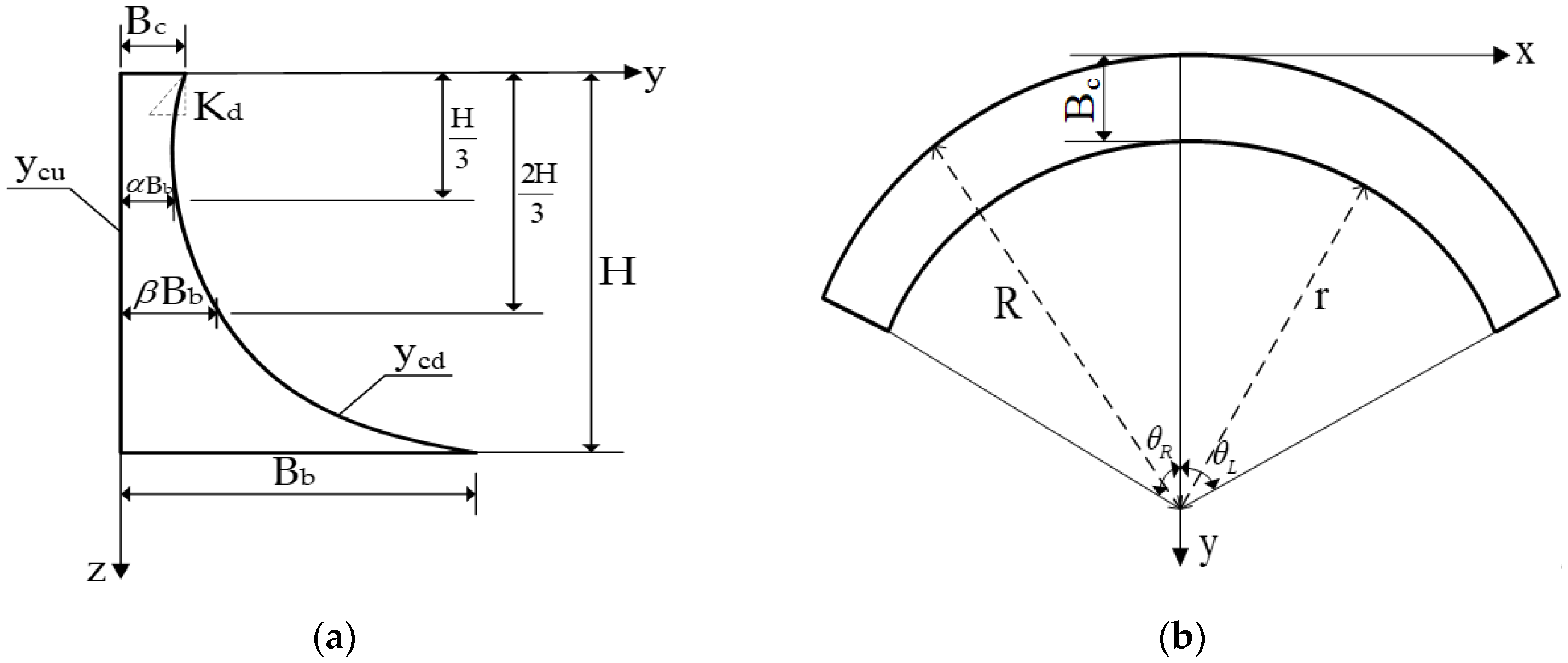
As shown in Figure 1a, if the upstream face curve ycu of the arch crown cantilever and the thickness B of the arch crown cantilever are determined, the downstream surface curve ycd can be determined, and the geometric structure of the arch crown cantilever can thus be obtained. The upstream surface curve ycu is a linear function of the z-axis, which can be expressed as follows:
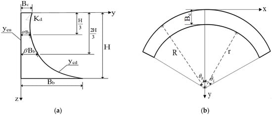
Figure 1.
Arch crown cantilever (a) and horizontal arch ring (b) of a single-curvature arch dam.
The thickness B is modeled as a cubic function of the z-axis and can be expressed as follows:
where b0, b1, b2, and b3 can be obtained by substituting four groups of control variables—z1 = 0, B1 = Bc; z2 = H/3, B2 = αBb; z3 = 2H/3, B3 = βBb; and z4 = H, B4 = Bb—into Equation (2). zi (i = 1, 2, 3, 4) is the distance extending vertically downward from the crest of the dam, and Bi (i = 1, 2, 3, 4) is the thickness of the arch crown cantilever at zi. Bc and Bb are the crest and bottom widths of the arch crown cantilever, respectively, and α and β are coefficients. H is the maximum height of the arch dam. Therefore, the curve ycd of the downstream surface of the arch crown cantilever can be obtained using Equations (1) and (2).
2.1.2. Horizontal Arch Ring
As illustrated in Figure 1b, the inner radius r of the horizontal arch ring can be determined as follows:
where R(z) is the outer radius of the horizontal arch circle. This study considered that the outer radius of the arch circle would not change with the height of the arch dam. After determining the inner radius r(z), we could derive the size of the horizontal arch ring by using the right-half central angle θR and the left-half central angle θL. Eight arch rings were selected along the height of the arch dam; therefore, 16 parameters—θR1, …, θR8, θL1, …, and θL8—were available to determine the size of the horizontal arch.
If the values of the 4 variables Bc, Bb, α, and β and 16 parameters θR1, …, θR8, θL1, …, and θL8 are determined, the geometry and size of the single-curvature arch dam can be determined.
2.2. Construction of Mathematical Optimization Model
On the basis of the geometric model established in Section 2.1, this study constructed a mathematical model for the design optimization of single-curvature arch dams. Our objective was to minimize the volume of arch dams while meeting the safety requirements of single-arch dams. The design variables, objective functions, and constraints are described in detail as follows.
2.2.1. Design Variables and Objective Function
The geometry of arch dams can be established using the variables mentioned in Section 2.1.
This study considered the volume V of a single-curvature arch dam as the objective function. In a finite element program, such as ANSYS, the volume V of a dam is the sum of the volumes of all finite elements, and V is also a function of the design variable X.
2.2.2. Constraints
Geometric constraints, stress constraints, and stability constraints should be considered in the design optimization of a single-curvature arch dam to meet engineering safety requirements.
Geometrical constraints. To facilitate construction, the degrees of overhang of the upstream and downstream surfaces of a single-curvature arch dam should be limited. The degree of overhang can be expressed as follows:
where Ku and Kd are the real maximal degrees of overhang of the upstream and downstream surfaces of the arch dam, respectively. These degrees must satisfy the following conditions:
where [Ku] and [Kd] are the allowable maximal degrees of overhang of the upstream and downstream surfaces, respectively. Following the Code for Design of Concrete Arch Dams, [Ku] = [Kd] = 0.3 in this study.
Stress constraints. Under the actions of gravitational load, hydrostatic pressure, uplift pressure, silt pressure, and temperature load, the principal stresses at each control point of an arch dam must satisfy the following conditions:
where σ1 and σ3 represent the first principal stress and the third principal stress, respectively. Moreover, the maximum value of σ1 and the minimum value of σ3 were used in this study. [σ1] and [σ3] denote the allowable values of the principal tensile stress and the principal compressive stress, respectively. This study used the FEM to analyze the structure of an arch dam. According to the Code for Design of Concrete Arch Dams, the equivalent stress should be calculated as follows:
where σ1eqv is the maximum equivalent stress and σ3eqv is the minimum equivalent stress. [σ1eqv] and [σ3eqv] are the allowable values of the maximum equivalent stress and the minimum equivalent stress, respectively. According to practical engineering design requirements, this study set the values of [σ1eqv] and [σ3eqv] to be equal to those of [σ1] and [σ3].
Stability constraints. Stability constraints can be divided into three types: safety factor constraint of anti-sliding stability, thrust angle constraint of the arch abutment, and center angle constraint of the arch ring. In this study, the center angle of the arch ring was limited,
where φ is the real central angle of the arch; φ = θL + θR, where the definitions of θR and θL are the same as those mentioned previously. [φ] is the largest allowable central angle of the arch.
In this study, the values of σ1, σ3, σ1eqv, σ3eqv, and V were calculated using ANSYS.
2.3. Solution of Mathematical Optimization Model
This study applied the GA-FEM, GA-KSM, and GA-SKSM to solve the optimization model. For the GA-FEM, the experiments required by the GA are performed in ANSYS software to solve the model. For the GA-KSM, before the start of genetic operations, the KSMs , , , , and of σ1, σ3, σ1eqv, σ3eqv, and V, respectively, satisfying the accuracy requirements were constructed; subsequently, the optimization models were solved using the GA based on these KSMs. For the GA-SKSM, the KSMs were first constructed based on small samples; subsequently, new samples guided by the infill criteria were obtained using the GA. These new samples were filled into the sample set to update the KSMs until the accuracy of the KSMs matched the requirements.
2.3.1. Genetic Algorithm
A GA is a heuristic algorithm that simulates the natural evolution process to find the optimal solution. GAs have strong robustness and global search ability [17,18,19,20,21]. Therefore, this study employed a GA to solve the optimization models. The design variables of the employed GA were coded using real numbers. Infeasibility degree (IFD)-based selections [22] were performed to manage the constraints involved in the optimization problem.
When the GA-FEM was used to solve the optimization model, the experiments required by the GA are performed in ANSYS to calculate σ1, σ3, σ1eqv, σ3eqv, and V, thus resulting in an extremely high calculation cost. Accordingly, the KSMs of σ1, σ3, σ1eqv, σ3eqv, and V could be constructed using a certain number of samples, after which the KSM-based GA could be used to solve the optimization model to improve optimization efficiency.
2.3.2. Kriging Surrogate Model
A KSM essentially uses the response information of known points to predict the response information of unknown points. The general steps involved in constructing a KSM are as follows. The first step is sampling. Sampling methods (such as central composite design, orthogonal experimental design, uniform design, and Latin hypercube sampling) can be used to generate samples of the design variables. The second step is KSM construction. A set of input–output data can be obtained by analyzing samples using a high-precision analysis model (e.g., ANSYS). Subsequently, a KSM can be constructed by fitting the input–output relationship of these sample data. The third step is accuracy evaluation.
Sampling methods. Common sampling methods include central composite design, orthogonal experimental design, uniform design, Latin hypercube sampling (LHS), and inherited LHS (ILHS). LHS [23] is easy to implement and has good consistency; therefore, it is widely used. ILHS [24] can improve the sampling efficiency and ensure the uniformity of LHS. In this study, ILHS was used in the GA-KSM for sample collection.
Constructing KSM. The general mathematical expression of a KSM is as follows:
where X is a vector of design variables; Φ (ε, X) is the polynomial regression model, generally a zero-, first-, or second-order polynomial; ε is the regression coefficient; f(X) is the basic function; and m(X) is a stochastic process and has the following statistical properties:
where is the constant process variance, Q(θ, Xi, Xj) is a correlation function of Xi, Xj, and θ. The Gaussian function presented in the following formula is commonly used as a correlation function:
where Xik and Xjk are the kth components of the training samples Xi and Xj, respectively. θk represents the kth element of the correlation vector parameter θ. The response values of each sample can then be subjected to linear weighted superposition interpolation to calculate the response values of unknown samples:
where w(X) = (w1, w2, …, wn)T is the weighting factor to be determined, and G = (g1, g2, …, gn)T. Based on the unbiased estimation condition, the following KSM expression can be obtained through collation:
where ε* = (FTQ−1F)−1FTQ−1G, γ* = Q−1(G−Fε*), ε* and γ* are fixed values and q = (Q(θ, X, X1), …, Q(θ, X, Xn))T. F is the regression matrix.
Accuracy evaluation. Accuracy evaluation is essential for determining whether a KSM is credible. If the accuracy meets the required threshold, the KSM can be used instead of FEM in the optimization process; otherwise, the KSM should be reconstructed through the addition of sample points. In this study, the maximum absolute relative error (MARE) was used to evaluate the accuracy of the KSM. MARE can be defined as follows:
where g and denote the actual value and predicted value, respectively, and n denotes the number of evaluation samples.
When a GA-KSM is used to solve optimization models, numerous samples are required to establish a KSM while satisfying the accuracy requirements over the entire design space. However, on the basis of a KSM constructed using a small set of samples, an optimized SKSM can be constructed by collecting samples from the domain of interest according to a reasonable infill criterion; this can further improve the efficiency of solving optimization models.
2.3.3. Sequential KSM
In an SKSM, the infill criterion is the key factor affecting model performance. To balance the global search ability against the convergence speed of the optimization algorithm, this study combined the MP strategy [25] with the LCB strategy [26] to construct the SKSM by using sample points obtained from the domain of interest in each optimization iteration.
MP criterion. The principle of the MP criterion is to find the minimum value of the objective function directly in a surrogate model and take the point that minimizes the value of the objective function as a new sample. Mathematically, the MP criterion can be expressed as follows:
where and are a surrogate model of the objective function and a constraint function, respectively. XL and XU are the lower and upper bounds of the design variable X, respectively. Nc is the number of constrained functions.
LCB criterion. To fully explore the optimal value of the objective function over the entire design space, the point that minimizes the LCB value can be taken as a new sample. The LCB function can be defined as follows:
where A is a constant and plays a major role in balancing global search and local search. According to the results of Liu et al. [27], we set A to 2. is the value predicted using the KSM, and s(X) is the standard deviation from the KSM.
2.3.4. Optimization Procedure
GA-FEM optimization procedure. When the GA-FEM was used to solve the optimization model, the experiments required by the GA are performed in ANSYS to calculate σ1, σ3, σ1eqv, σ3eqv, and V. The convergence criteria (CC) of GA-FEM is defined as follows:
where gen and gen′ are numbers of a generation of GA, and Vgen and Vgen′ are the best objective values for the corresponding generation. When CC ≤ 1%, then GA-FEM is considered to converge to the optimal solution.
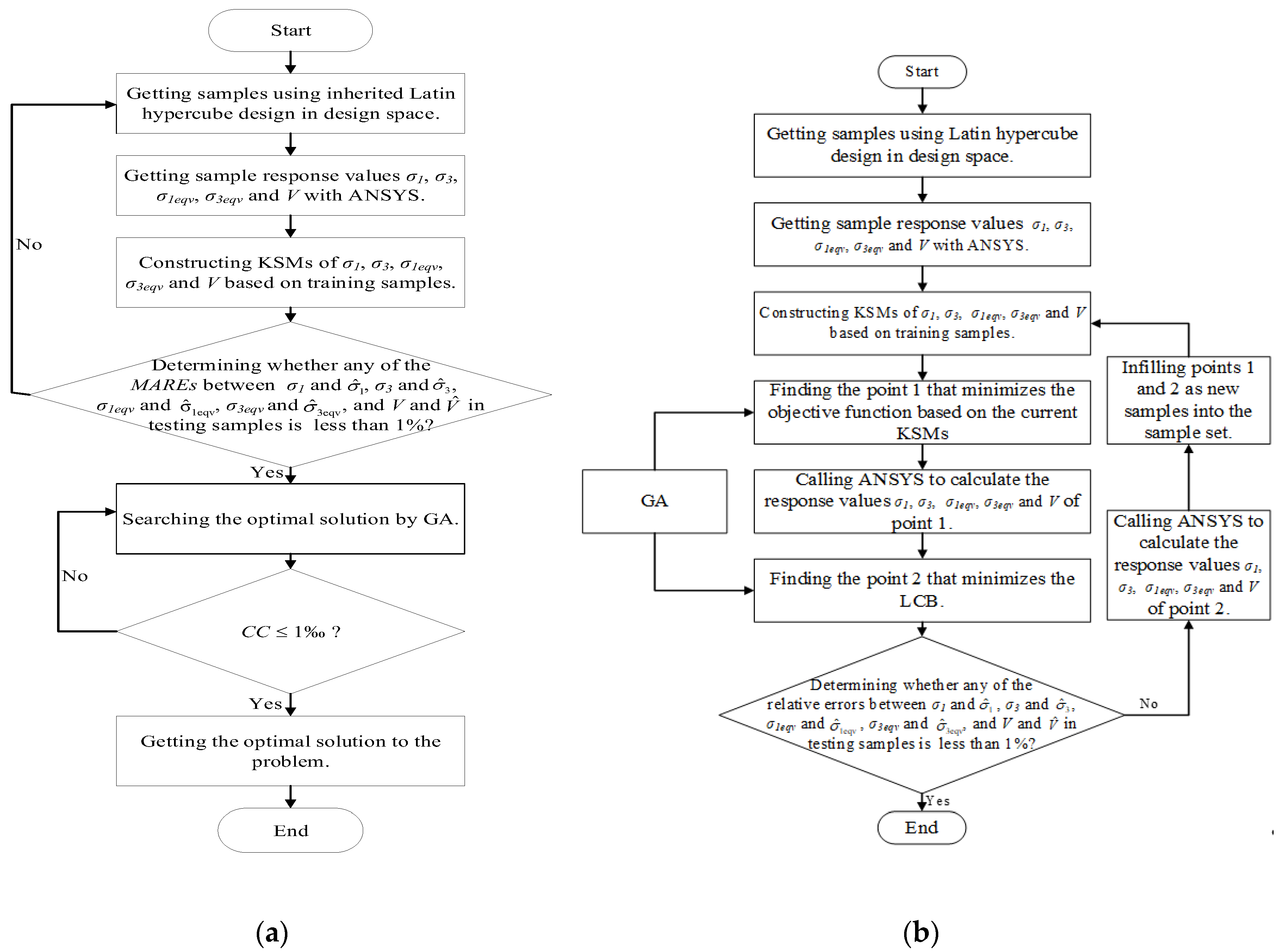
GA-KSM optimization procedure. To improve sampling efficiency, this study collected samples in the design space by using ILHS. Of the collected samples, 80% were used to construct the KSMs of σ1, σ3, σ1eqv, σ3eqv, and V, and 20% were used to evaluate the accuracy of these KSMs. Subsequently, the study determined whether any of the MAREs between σ1 and , σ3 and , σ1eqv and , σ3eqv and , and V and were less than 1%. If none of the MAREs were less than 1%, 50 samples were added to the sample set using the same method until the KSMs satisfied the accuracy requirements. The mathematical model of arch dam optimization was then solved using the GA. When CC ≤ 1‰, the optimization was terminated. A flowchart of the GA-KSM is illustrated in Figure 2a.
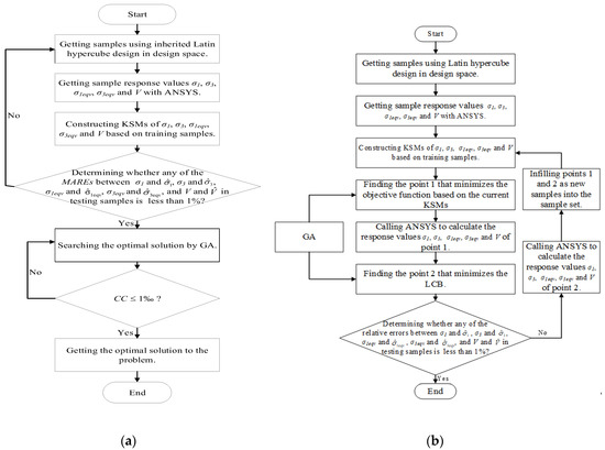
Figure 2.
Schematic flowchart of (a) a genetic algorithm with a Kriging surrogate model (GA-KSM) and (b) a genetic algorithm with a sequential Kriging surrogate model (GA-SKSM).
GA-SKSM optimization procedure. First, before the optimization process was initiated, LHS was applied to collect 50 samples to construct the KSMs. Second, the GA was used to find point 1 minimizing the value of the objective function (when CC ≤ 1‰, then GA is considered to converge to the optimal solution). Meanwhile, the values of , , , , and can be obtained. The response values σ1, σ3, σ1eqv, σ3eqv, and V of point 1 were calculated using ANSYS. Third, the GA was used to find point 2 minimizing the value of LCB (when CC ≤ 1‰, then GA is considered to converge to the optimal solution). Fourth, the study determined whether any of the relative errors between σ1 and , σ3 and , σ1eqv and , σ3eqv and , and V and were smaller than 1%; if none of the relative errors were less than 1%, the response values σ1, σ3, σ1eqv, σ3eqv, and V of point 2 were calculated using ANSYS. So, in each iteration, point 1, point 2, and their response values were infilled into the existing sample set collectively to update the KSM until the entire optimization process converged. A flowchart of the optimization process is displayed in Figure 2b.
3. Case Study
3.1. Basic Information of a Single-Curvature Arch Dam
To investigate the computational efficiency of the GA-FEM, GA-KSM, and GA-SKSM for shape optimization of a single-curvature arch dam, this study used the Jiancaogou single-curvature arch dam, located approximately 160 m upstream of the Jiancaogou Bridge in Guizhou, China, as a test example. The maximum height of this dam is 55.5 m, upstream water level is 53 m, and sedimentation water level is 38 m.
In this study, four variables were defined for optimizing the geometry of this single-curvature arch dam. The lower and upper bounds of these design variables required in the optimization process are listed in Table 1.

Table 1.
Lower and upper bounds of design variables.
Moreover, to determine the optimal shape of the single-curvature arch dam, the mechanical properties of the dam body and foundation rock materials listed in Table 2 were considered.
Table 2.
Properties of dam body and foundation rock.
3.2. Finite Element Model Establishing and Parameter Setting
This study used finite elements to separate the concrete and bedrock of the single-curvature arch dam. Moreover, the study established a three-dimensional (3D) finite element model of the arch dam (Figure 3) by using ANSYS in order to calculate the values of σ1, σ3, σ1eqv, σ3eqv, and V. The dam body was discretized using 20-node elements, with each node having three degrees of freedom. All elements used in this study were linear solid. The horizontal grid extended by 1.5 times the dam height, whereas the vertical grid extended by 1 times the dam height and penetrated into the bedrock. The loads involved were gravity load, hydrostatic pressure, uplift pressure, silt pressure, and temperature load.
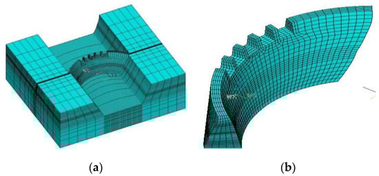
Figure 3.
(a) Finite element model of the foundation rock system of the Jiancaogou single-curvature arch dam. (b) Finite element model of the dam body.
The population size of the GA was set to 50, and the maximum generation was set to 100. The crossover probability was set to 0.7, and the mutation probability was set to 0.01.
3.3. Optimization Results and Discussion
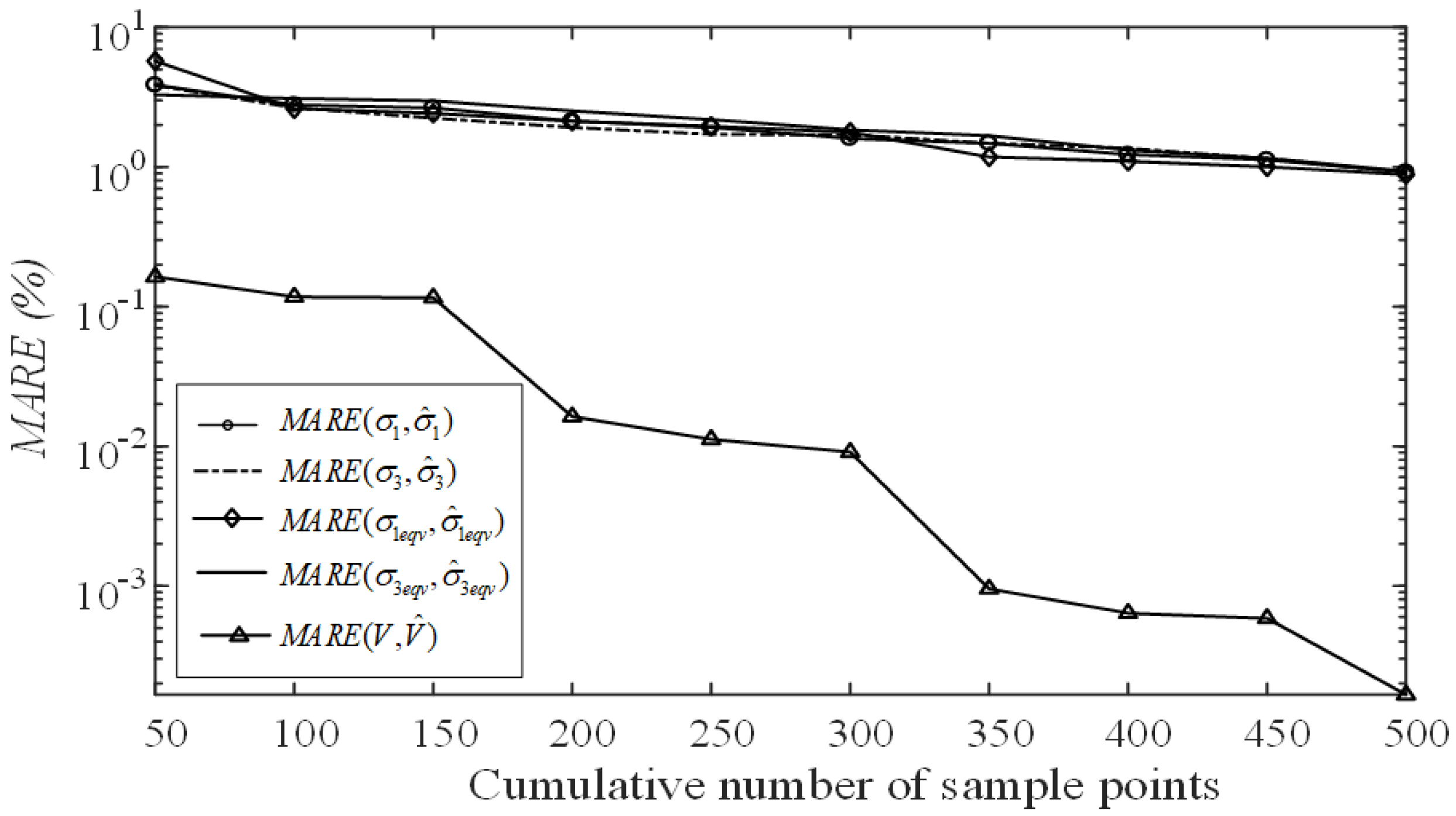
When a GA-KSM was used to optimize the shape of a single-curvature arch dam, the optimization results depended predominantly on the approximate accuracy of the KSM, which is directly related to the number of training samples. In this study, to meet the accuracy requirements of the KSMs of σ1, σ3, σ1eqv, σ3eqv, and V, any of the MAREs between σ1 and , σ3 and , σ1eqv and , σ3eqv and , and V and must not exceed 1%. Figure 4 illustrates the variation of MAREs between σ1 and , σ3 and , σ1eqv and , σ3eqv and , and V and with the number of sample points increasing.
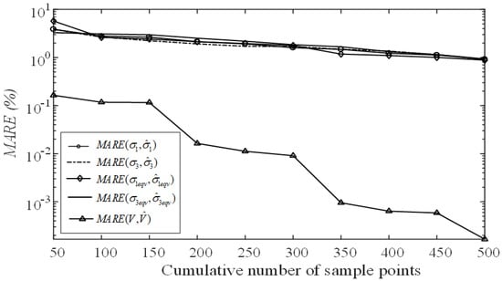
Figure 4.
The variation of the maximum absolute relative errors (MAREs) between σ1 and , σ3 and , σ1eqv and , σ3eqv and , and V and with the number of sample points increasing.
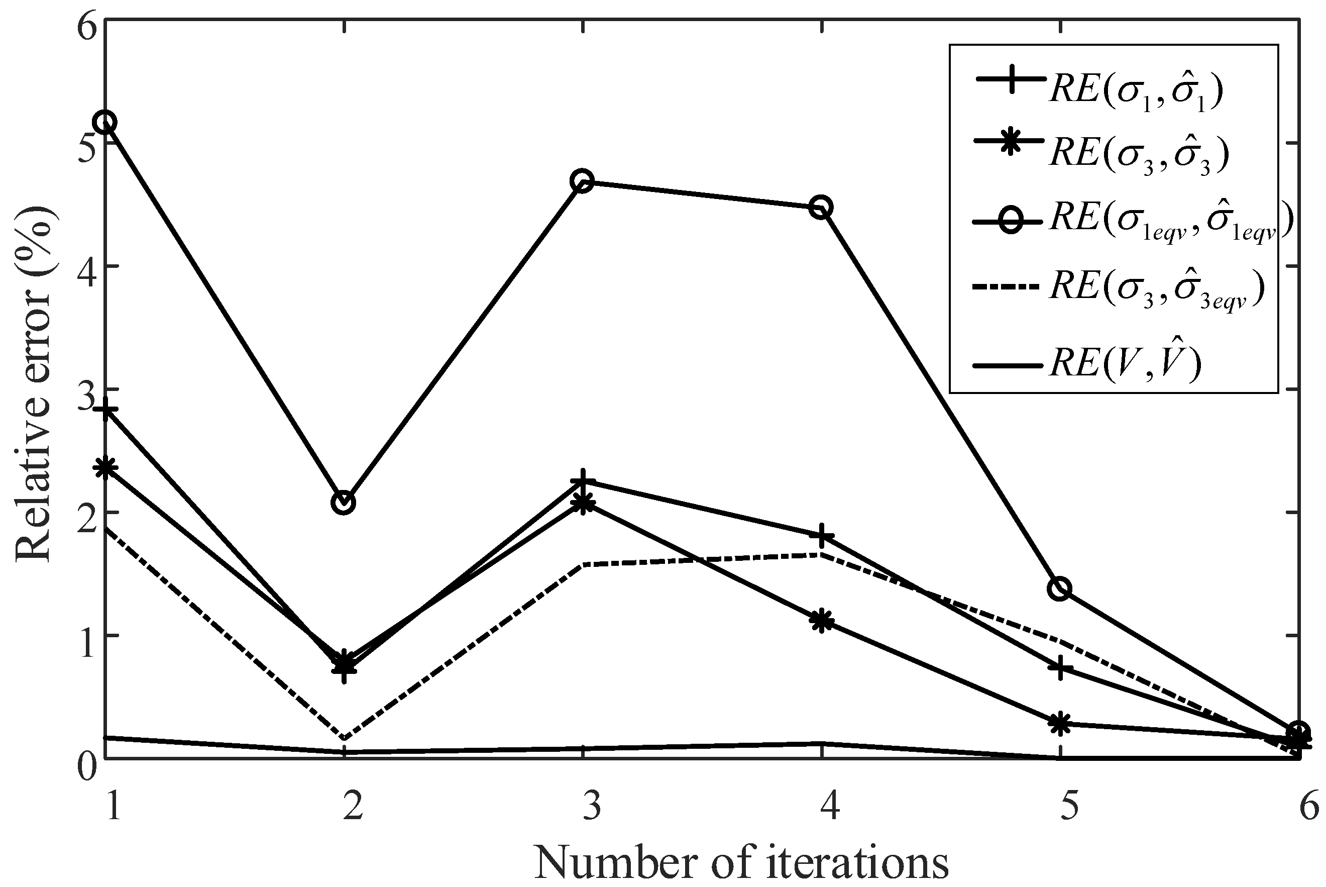
As illustrated in Figure 4, the MAREs between σ1 and , σ3 and , σ1eqv and , σ3eqv and , and V and decreased as the sample size increased. When the accuracy of these KSMs satisfied the requirements, the number of training samples was 500. Such a high sampling cost is unacceptable in engineering optimization problems. Figure 5 depicts the variation of relative errors (RE) between σ1 and , σ3 and , σ1eqv and , σ3eqv and , and V and in GA-SKSM with number of the iterations increasing.
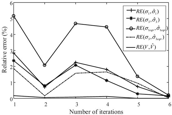
Figure 5.
The variation of relative errors between σ1 and , σ3 and , σ1eqv and , σ3eqv and , and V and involved in GA-SKSM with number of iterations increasing.
As the number of iterations increased, in other words, as the samples in the initial sample set of KSM increased, the relative errors between σ1 and , σ3 and , σ1eqv and , σ3eqv and , and V and generally decreased, but this reduction was volatile (Figure 5). This volatility can be ascribed to the fact that new optimal solutions were discovered continuously in the process of infilling new samples into the sample set. When the optimal solution tended to be stable, the relative errors between σ1 and , σ3 and , σ1eqv and , σ3eqv and , and V and decreased gradually until the convergence criteria were satisfied. This indicates that upon application of the MP criterion and the LCB criterion, the algorithm collected sample points from the region of interest only, and finally, the SKSM achieved high approximation accuracy in the region of interest. Table 3 presents a summary of the optimal designs of the single-curvature arch dam obtained using the GA-FEM, GA-KSM, and GA-SKSM.
Table 3.
Optimal designs of the single-curvature arch dam obtained using the generic algorithm finite element method (GA-FEM), GA-KSM, and GA-SKSM.
As shown in Table 3, for optimizing the single-curvature arch dam example considered in this study, the GA-FEM and GA-KSM required 1150 and 500 numerical simulations, respectively. It is noteworthy that the number of numerical simulations (62 numerical simulations (i.e., 62 samples) included 50 samples required to construct the initial KSM and 12 samples obtained by GA to improve the accuracy of KSM under the guidance of the LCB criterion and MP criteria) required by the GA-SKSM was 5.40% and 12.40% of the number of simulations required by the GA-FEM and GA-KSM, respectively, and the volume V of the arch dam based on GA-SKSM is the minimum. This demonstrates that the GA-SKSM can guarantee high accuracy near the optimal solution with fewer samples and can converge approximately to the optimal solution. Therefore, the GA-SKSM is superior to the other two algorithms in terms of optimization efficiency and results.
This study considered only a simple single-curvature arch dam. Hence, complex arch dams should be considered in future studies.
4. Conclusions
To improve the calculation efficiency of FEM-based design optimization of a single-curvature arch dam and the prediction accuracy of a KSM, an SKSM was constructed using the MP criterion and LCB criterion. Accordingly, the shape of the single-curvature arch dam was optimized by combining a GA with the SKSM. Compared with the traditional arch dam design method based on the FEM and KSM, the GA-SKSM could significantly reduce the number of finite element numerical calculation and the number of sampling points, in addition to improving the calculation efficiency. The GA-SKSM in this study can be applied to efficiently addressing the design optimization problem of arch dams, and it has practical engineering value.
Author Contributions
Research conceptualization, Y.-Q.W., R.-H.Z. and X.-Y.M.; data curation, Y.-Q.W., R.-H.Z. and X.-Y.M.; methodology, Y.-Q.W., Y.L. and Y.-Z.C.; writing—original draft, Y.-Q.W.; writing—review & editing, X.-Y.M.
Funding
This research was funded by the National Key R&D Program of China (No. 2017YFC0403202) and the National Science and Technology Support Program of China (No. 2015BAD24B02).
Conflicts of Interest
The authors declare no conflicts of interest.
References
- Pourbakhshian, S.; Ghaemain, M. Shape Optimization of Arch Dams Using Sensitivity Analysis. KSCE J. Civ. Eng. 2016, 20, 1966–1976. [Google Scholar] [CrossRef]
- Rita, M.; Fairbairn, E.; Ribeiro, F.; Andrade, H.; Barbosa, H. Optimization of Mass Concrete Construction Using a Twofold Parallel Genetic Algorithm. Appl. Sci. 2018, 8, 399. [Google Scholar] [CrossRef]
- Tan, F.J.; Lahmer, T. Shape Optimization Based Design of Arch-Type Dams under Uncertainties. Eng. Optimiz. 2018, 50, 1470–1482. [Google Scholar]
- Sukkarak, R.; Jongpradist, P.; Pramthawee, P. A Modified Valley Shape Factor for the Estimation of Rockfill Dam Settlement. Comput. Geotech. 2019, 108, 244–256. [Google Scholar] [CrossRef]
- Wang, G.G.; Shan, S. Review of Metamodeling Techniques in Support of Engineering Design Optimization. J. Mech. Des. 2007, 129, 370–380. [Google Scholar] [CrossRef]
- Mahani, A.S.; Shojaee, S.; Salajegheh, E.; Khatibinia, M. Hybridizing Two-Stage Meta-Heuristic Optimization Model with Weighted Least Squares Support Vector Machine for Optimal Shape of Double-Arch Dams. Appl. Soft Comput. 2015, 27, 205–218. [Google Scholar] [CrossRef]
- Chang, C.M.; Lin, T.K.; Chang, C.W. Applications of Neural Network Models for Structural Health Monitoring Based on Derived Modal Properties. Measurement 2018, 129, 457–470. [Google Scholar] [CrossRef]
- Jamli, M.R.; Farid, N.M. The Sustainability of Neural Network Applications within Finite Element Analysis in Sheet Metal Forming: A Review. Measurement 2019, 138, 446–460. [Google Scholar] [CrossRef]
- Krige, D.G. A Statistical Approach to Some Basic Mine Valuation Problems on the Witwatersrand. J. South. Afr. Inst. Min. Metall. 1994, 94, 95–111. [Google Scholar]
- Putra, N.K.; Palar, P.S.; Anzai, H.; Shimoyama, K.; Ohta, M. Multiobjective Design Optimization of Stent Geometry with Wall Deformation for Triangular and Rectangular Struts. Med. Biol. Eng. Comput. 2019, 57, 15–26. [Google Scholar] [CrossRef]
- Gaspar, B.; Teixeira, A.P.; Soares, C.G. Assessment of the Efficiency of Kriging Surrogate Models for Structural Reliability Analysis. Probabilist. Eng. Mech. 2014, 37, 24–34. [Google Scholar] [CrossRef]
- Zhang, G.Q.; Yang, H.T. An Approximate Solution for the Bimodular Plane Problem Based on Kriging Surrogate Model. Eng. Mech. 2013, 30, 23–27. [Google Scholar]
- Liu, Y.S.; Wang, X.J.; Wang, L. A Dynamic Evolution Scheme for Structures with Interval Uncertainties by Using Bidirectional Sequential Kriging Method. Comput. Methods Appl. Mech. Eng. 2019, 348, 712–729. [Google Scholar]
- Cheng, J.; Jiang, P.; Zhou, Q.; Hu, J.X.; Yu, T.; Shu, L.S.; Shao, X.Y. A Lower Confidence Bounding Approach Based on the Coefficient of Variation for Expensive Global Design Optimization. Eng. Comput. 2019, 36, 830–849. [Google Scholar] [CrossRef]
- Raponi, E.; Bujny, M.; Olhofer, M.; Aulig, N.; Boria, S.; Duddeck, F. Kriging-Assisted Topology Optimization of Crash Structures. Comput. Methods Appl. Mech. Eng. 2019, 348, 730–752. [Google Scholar] [CrossRef]
- Song, C.; Yang, X.D.; Song, W.P. Multi-Infill Strategy for Kriging Models Used in Variable Fidelity Optimization. Chin. J. Aeronaut. 2018, 31, 448–456. [Google Scholar] [CrossRef]
- Salmasi, F. Design of Gravity Dam by Genetic Algorithms. World Acad. Sci. Eng. Technol. 2011, 56, 864–869. [Google Scholar]
- Babbar-Sebens, M.; Minsker, B.S. Interactive Genetic Algorithm with Mixed Initiative Interaction for Multi-Criteria Ground Water Monitoring Design. Appl. Soft Comput. 2012, 12, 182–195. [Google Scholar] [CrossRef]
- Li, M.G.; Li, M.; Han, G.P.; Liu, N.; Zhang, Q.M.; Wang, Y. Optimization Analysis of the Energy Management Strategy of the New Energy Hybrid 100% Low-Floor Tramcar Using a Genetic Algorithm. Appl. Sci. 2018, 8, 1144. [Google Scholar] [CrossRef]
- Prasanchum, H.; Kangrang, A. Optimal Reservoir Rule Curves under Climatic and Land Use Changes for Lampao Dam Using Genetic Algorithm. KSCE J. Civ. Eng. 2018, 22, 351–364. [Google Scholar] [CrossRef]
- Yoo, J.W.; Ronzio, F.; Courtois, T. Road Noise Reduction of a Sport Utility Vehicle Via Panel Shape and Damper Optimization on the Floor Using Genetic Algorithm. Int. J. Automot. Technol. 2019, 20, 1043–1050. [Google Scholar] [CrossRef]
- Zhang, J.M.; Xie, L. Particle Swarm Optimization Algorithm for Constrained Problems. Asia Pac. J. Chem. Eng. 2009, 4, 437–442. [Google Scholar] [CrossRef]
- Kim, J.B.; Hwang, K.Y.; Kwon, B.I. Optimization of Two-Phase in-Wheel Ipmsm for Wide Speed Range by Using the Kriging Model Based on Latin Hypercube Sampling. IEEE. Trans. Magn. 2011, 47, 1078–1081. [Google Scholar] [CrossRef]
- Wang, G.G. Adaptive Response Surface Method Using Inherited Latin Hypercube Design Points. J. Mech. Des. 2003, 125, 210–220. [Google Scholar] [CrossRef]
- Parr, J.M.; Keane, A.J.; Forrester, A.I.J.; Holden, C.M.E. Infill Sampling Criteria for Surrogate-Based Optimization with Constraint Handling. Eng. Optimiz. 2012, 44, 1147–1166. [Google Scholar] [CrossRef]
- Yang, Z.B.; Zhou, J.Z.; Li, H.T.; Li, W.T.; Shi, X.W.; Wang, M. Design of Hexagonal Circularly Polarized Antenna Array Using Paralleled Dynamic Minimum Lower Confidence Bound. Int. J. RF Microw. Comput. Aided Eng. 2018, 28, e21184. [Google Scholar] [CrossRef]
- Liu, B.; Zhang, Q.; Fernandez, F.; Gielen, G. Self-Adaptive Lower Confidence Bound: A New General and Effective Prescreening Method for Gaussian Process Surrogate Model Assisted Evolutionary Algorithms. In Proceedings of the 2012 IEEE Congress on Evolutionary Computation, Brisbane, Australia, 10–15 June 2012. [Google Scholar]

© 2019 by the authors. Licensee MDPI, Basel, Switzerland. This article is an open access article distributed under the terms and conditions of the Creative Commons Attribution (CC BY) license (http://creativecommons.org/licenses/by/4.0/).