Dynamics of Double-Beam System with Various Symmetric Boundary Conditions Traversed by a Moving Force: Analytical Analyses

Abstract

Dynamics of the double-beam system under moving loads have been paid much attention due to its wide applications in reality from the analytical point of view but the previous studies are limited to the simply supported boundary condition. In this study, to understand the vibration mechanism of the system with various boundary conditions, the double-beam system consisted of two general beams with a variety of symmetric boundary conditions (fixed-fixed, pinned-pinned, fixed-pinned, pinned-fixed and fixed-free) under the action of a moving force is studied analytically. The closed-form frequencies and mode shapes of the system with various symmetric boundary conditions are presented by the Bernoulli-Fourier method and validated with Finite Element results. The analytical explicit solutions are derived by the Modal Superposition method, which are verified with numerical results and previous results in the literature. As found, each wavenumber of the double-beam system is corresponding to two sub-modes of the system and the two sub-modes associated with the first wavenumber of the system both contribute significantly to the vibration of the system under a moving force. The analytical solutions indicate that the mass ratio, the bending stiffness ratio, the stiffness ratio of contact springs and the speed ratio of the moving force are the factors influencing the vibrations of the system under a moving force. The relationships between these dimensionless parameters and the displacement ratio of the system are investigated and presented in the form of plots, which could be referred in the design of the double-beam system.

1. Introduction

The double-beam system has wide applications in reality, such as floating-slab railway tracks [1], track-bridge systems [2,3], sandwich beams composed of an interconnected layer [4], vibration absorbers [5,6] and carbon nanotubes [7]. Studying modal properties (frequencies and mode shapes) of such a system contributes to understanding the mechanism of the system dynamics and lays the foundation for working out its dynamic response under external excitations by using Modal Superposition (MS) method. Seelig and Hoppmann II [8] presented the analytical frequencies and associated mode shapes of the elastically connected double-beam system consisting of two identical beams for the first time. Rao [9] studied the free vibrations of elastically connected parallel bars considering the effects of rotary inertia and shear deformation. Tadatake et al. [5] presented the natural frequencies and mode shapes of double-beam systems with two general beams by using a generalized method of finite integral transformation and the Laplace transformation. The same problem was also studied by Oniszczuk [10] by using the classic Bernoulli-Fourier method. Mirzabeigy et al. [11] presented explicit expressions for natural frequencies of double-beam systems with arbitrary boundary conditions. Han et al. [12] applied the dynamic stiffness method to establish the exact dynamic stiffness matrix and frequency equation for an axially-loaded double-beam system with arbitrary boundary conditions. The transcendental frequency equation was solved by an improved Wittrick-Williams algorithm. Hao et al. [13] investigated the free vibrations of double-beam systems with arbitrary boundary conditions by a modified Fourier-Ritz approach.

Compared with the vibrations of a single beam under moving loads [14,15,16,17], the vibrations of double-beam systems excited by moving loads are more complicated and have drawn much attention recently. The vibrations of a simply supported double-beam system with two identical beams interconnected by an elastic layer under the action of a fixed harmonic force were solved in the closed-form solutions by Vu et al. [18]. The connecting damping between two beams was ignored. The vibrations of the same system subjected to a moving constant force [19], a moving harmonic force [20] were studied analytically. The system under the action of a moving oscillator [21] was also studied numerically. Zhang and Ma [22] investigated the influence of compressive axil loads on the vibration of the system. Kessel [23] studied the resonances of a simply supported double-beam system with two general beams excited by a cyclic moving load. The connecting damping between two beams was ignored, which was then considered in Reference [24]. The analytical solutions for the forced vibrations of the same system were presented by Oniszczuk [25]. Chonan [26] investigated the vibration of a double-beam system interconnected by elastic springs subjected to an impulse load considering the mass of the springs. Pavlović et al. [27] investigated the stability of a double-beam system subjected to random compressive axil forces. The forced vibration and buckling of a Rayleigh and Timoshenko double-beam system subjected to arbitrary continuous load with the effect of compressive axil loads were studied by Stojanović and Kozić [28]. Kozić et al. [29] analyzed the free vibration and buckling of a double-beam system under axial loading joined by a Kerr-type layer. It should be noticed that all these studies regarding forced vibrations of double-beam systems are restricted to simply supported double-beam systems.

Hamada et al. [5] pointed out the similarity between an elastically connected multi-beam system with same boundary conditions for all the beams (symmetric boundary conditions) and a multi-degree-of-freedom mass-spring system. The free vibrations of an elastically connected double-beam system, taking account of the axial forces on the beams were studied in References [30,31]. Li and Sun [32] presented a semi-analytical method to study the transverse vibration of an undamped elastically connected double-beam system with arbitrary boundary conditions. The transverse vibrations of a double-beam system interconnected by a viscoelastic layer were studied numerically [33]. The two beams can be restricted with different boundary conditions. Şimşek and Cansız [34] studied the vibrations of elastically connected double-functionally graded beam systems with different boundary conditions under the action of a moving harmonic load by a numerical method. Zhang et al. [35] developed an analytical framework to study the transverse vibrations of double-beam systems made of two parallel Timoshenko beams connected by springs and coupled with various discontinuities.

The free vibration, dynamic response and static buckling of an axially-loaded double-beam system with a viscoelastic layer were investigated by Chen and Sheu [36]. Li and Hua [37] introduced a spectral Finite Element method to study the vibrations of double-beam systems considering shear deformation and rotary inertia of the beams. The modal properties of the system were determined by applying the Muller root search algorithm. Palmeri and Adhikari [38] presented a Galerkin-type state-space approach for studying vibrations of a double-beam system interconnected by a viscoelastic layer. Various element matrixes for the double-beam systems were established, for example, in References [2,3,6,39,40].

In spite of the above studies about the forced vibrations of double-beam systems with various boundary conditions under the action of moving loads, to the author’s best knowledge, only analytical solutions for the forced vibration of simply supported double-beam system are available in the literature. To understand the vibration mechanism of the system with various boundary conditions, the vibrations of double-beam system with five general kinds of symmetric boundary conditions (fixed-fixed, pinned-pinned, fixed-pinned, pinned-fixed and fixed-free) excited by a moving force are investigated by an analytical approach in this paper. The closed-form expressions to the modal properties of the double-beam system with the various symmetric boundary conditions are presented in Section 2. Parametric studies are also conducted to investigate the influences of the order of basic modes, contact stiffness ratio, mass ratio and beam stiffness ratio on the modal properties of the double-beam systems in this section. The analytical solutions to the vibrations of the double-beam system with the various boundary conditions subjected to a moving force are derived in Section 3. The effects of speed ratio, contact stiffness ratio, mass ratio and beam stiffness ratio on the dynamic responses of the system are also studied in a dimensionless form in this section. Conclusions are drawn in Section 4.

2. Frequencies and Mode Shapes of the Double-Beam System

2.1. Mathematical Formulation

The double-beam system considered in this study is consisted of a primary beam ($w_1$) and an equal-length secondary beam ($w_2$) as shown in Figure 1. Both beams are taken to be Euler-Bernoulli beams. The two beams are interconnected with uniformly distributed springs of stiffness $k_{\mathrm{e}}$. The boundary conditions for the primary beam are the same as for the secondary beam (symmetric boundary conditions). Five general kinds of symmetric boundary conditions are considered in this section: fixed-fixed, pinned-pinned, fixed-pinned, pinned-fixed and free-free.

The equations of motion of the secondary beam and the primary beam can be expressed as:

$$E_2{I}_2{w}_2^{⁗}+{\rho }_2{A}_2{\ddot{w}}_2-k_{\mathrm{e}}\left(w_1-w_2\right)=0$$

(1)

$$s_{\mathrm{k}}{E}_2{I}_2{w}_1^{⁗}+s_{\mathrm{m}}{\rho }_2{A}_2{\ddot{w}}_1+k_{\mathrm{e}}\left(w_1-w_2\right)=0$$

(2)

where $s_{\mathrm{k}}=\frac{E_1{I}_1}{E_2{I}_2}$ and $s_{\mathrm{m}}=\frac{{\rho }_1{A}_1}{{\rho }_2{A}_2}$ are the beam stiffness ratio and mass ratio of the primary beam to the secondary beam, respectively.

Using the Bernoulli-Fourier method [41], the displacement of the two beams can be expressed as

$$\{\begin{array}{c}{w}_2\left(x,t\right)={\phi }_2\left(x\right)e^{i\omega t}\\ w_1\left(x,t\right)={\phi }_1\left(x\right)e^{i\omega t}\end{array}$$

(3)

where ${\phi }_1$ and ${\phi }_2$ are mode shapes of the primary beam and the secondary beam, respectively and $\omega$ is the natural frequency of the double-beam system.

Substituting Equation (3) into Equation (1), one can obtain the relationship between ${\phi }_1$ and ${\phi }_2$ as

$${\phi }_1=\frac{E_2{I}_2}{k_{\mathrm{e}}}{\phi }_2^{⁗}+\left(1-\frac{{\omega }^2{\rho }_2{A}_2}{k_{\mathrm{e}}}\right){\phi }_2$$

(4)

Substituting Equation (4) into Equation (2) and removing the term $e^{i\omega t}$ result in

$$a{\phi }_2^{\mathrm{VIII}}+b{\phi }_2^{\mathrm{IV}}+c{\phi }_2=0$$

(5)

where

$$\begin{gathered} a=\frac{S_{\mathrm{k}}{\left(E_2{I}_2\right)}^2}{k_{\mathrm{e}}} \\ b=⎡\left(s_{\mathrm{k}}{E}_2{I}_2-\frac{s_{\mathrm{k}}{E}_2{I}_2{\omega }^2{\rho }_2{A}_2}{k_{\mathrm{e}}}\right)+\left(k_{\mathrm{e}}-{\omega }^2{S}_{\mathrm{m}}{\rho }_2{A}_2\right)\frac{E_2{I}_2}{k_{\mathrm{e}}}⎤ \\ c=\left(-{\omega }^2{\rho }_2{A}_2+\frac{s_{\mathrm{m}}{\left({\omega }^2{\rho }_2{A}_2\right)}^2}{k_{\mathrm{e}}}-{\omega }^2{s}_{\mathrm{m}}{\rho }_2{A}_2\right) \end{gathered}$$

(6)

The general solution of Equation (5) is

$${\phi }_2\left(x\right)=C_1{e}^{r_{1}x}+C_2{e}^{r_{2}x}+C_3{e}^{r_{3}x}+C_4{e}^{r_{4}x}+C_5{e}^{r_{5}x}+C_6{e}^{r_{6}x}+C_7{e}^{r_{7}x}+C_8{e}^{r_{8}x}$$

(7)

where $C_i$ ($i=1,2,\dots 8$) are unknown coefficients and $r_i$ ($i=1,2,\dots 8$) are the roots of the characteristic equation of Equation (5)

$$a{r}^8+b{r}^4+c=0$$

(8)

Substituting Equation (6) into Equation (8) and taking $\omega$ as the unknown result in

$$\begin{gathered} {\omega }_n^{\left(1\right)}=\frac{{\tilde{\omega }}_{2,n}}{\sqrt{2}}\sqrt{\left(1+\frac{s_{\mathrm{k}}}{s_{\mathrm{m}}}\right)+\left(1+\frac{1}{s_{\mathrm{m}}}\right)\frac{s_{\mathrm{e}}}{{\left(r^{\left(n\right)}l\right)}^4}-\sqrt{{\left[\left(1-\frac{s_{\mathrm{k}}}{s_{\mathrm{m}}}\right)+\left(1-\frac{1}{s_{\mathrm{m}}}\right)\frac{s_{\mathrm{e}}}{{\left(r^{\left(n\right)}l\right)}^4}\right]}^2+\frac{4s_{\mathrm{e}}^2}{s_{\mathrm{m}}{(r^{\left(n\right)}l)}^8}}} \\ {\omega }_n^{\left(2\right)}=\frac{{\tilde{\omega }}_{2,n}}{\sqrt{2}}\sqrt{\left(1+\frac{s_{\mathrm{k}}}{s_{\mathrm{m}}}\right)+\left(1+\frac{1}{s_{\mathrm{m}}}\right)\frac{s_{\mathrm{e}}}{{\left(r^{\left(n\right)}l\right)}^4}+\sqrt{{\left[\left(1-\frac{s_{\mathrm{k}}}{s_{\mathrm{m}}}\right)+\left(1-\frac{1}{s_{\mathrm{m}}}\right)\frac{s_{\mathrm{e}}}{{\left(r^{\left(n\right)}l\right)}^4}\right]}^2+\frac{4s_{\mathrm{e}}^2}{s_{\mathrm{m}}{\left(r^{\left(n\right)}l\right)}^8}}} \end{gathered}$$

(9)

where $s_{\mathrm{e}}$ is the contact stiffness ratio which is a dimensionless stiffness ratio defined as follows:

$$s_{\mathrm{e}}=\frac{k_{\mathrm{e}}{l}^4}{E_2{I}_2}$$

(10)

and

$${\tilde{\omega }}_{2,n}={(r^{\left(n\right)})}^2\sqrt{\frac{E_2{I}_2}{{\rho }_2{A}_2}}$$

(11)

$r^{\left(n\right)}l$ represents the $n\mathrm{th}$ wavenumber of the double-beam system and it is a constant depending on the boundary conditions of the double-beam system. It will be shown below that the wavenumbers of the double-beam systems are the same as those for a single beam if the boundary conditions of the primary beam are the same as the secondary beam (symmetric boundary conditions). Therefore, Equation (11) also represents the nth natural frequency of a single secondary beam.

It can be seen from Equation (9) that two sub-modes of the double-beam system are corresponding to one wavenumber of the double-beam system. The order of the wavenumber of the double-beam system is defined as the basic mode number in the following context.

The following relationship can be obtained from Equation (8)

$$\{\begin{array}{c}{r}_2=-r_1,r_3=r_{1}i,r_4=-r_{1}i\\ r_6=-r_5,r_7=r_{5}i,r_8=-r_{5}i\end{array}$$

(12)

Substituting Equation (12) into Equation (7) results in

$${\phi }_2\left(x\right)=C_1{e}^{r_{1}x}+C_2{e}^{-r_{1}x}+C_3{e}^{i{r}_{1}x}+C_4{e}^{-i{r}_{1}x}+C_5{e}^{r_{5}x}+C_6{e}^{-r_{5}x}+C_7{e}^{i{r}_{5}x}+C_8{e}^{-i{r}_{5}x}$$

(13)

2.1.1. Fixed-Fixed Boundary Conditions

The boundary stiffness is

$$\{\begin{array}{c}{k}_{\mathrm{v},1}=k_{\mathrm{v},2}=\infty \\ k_{\mathrm{r},1}=k_{\mathrm{r},2}=\infty \end{array}$$

(14)

The boundary conditions of the fixed-fixed double-beam system are

$$\{\begin{array}{c}\begin{array}{c}{\phi }_1\left(0\right)=0\\ {\phi }_1^{\prime }\left(0\right)=0\end{array}\\ \begin{array}{c}{\phi }_1\left(l\right)=0\\ {\phi }_1^{\prime }\left(l\right)=0\end{array}\end{array},\{\begin{array}{c}\begin{array}{c}{\phi }_2\left(0\right)=0\\ {\phi }_2^{\prime }\left(0\right)=0\end{array}\\ \begin{array}{c}{\phi }_2\left(l\right)=0\\ {\phi }_2^{\prime }\left(l\right)=0\end{array}\end{array}$$

(15)

Substituting Equation (15) into Equations (4) and (13) results in an equation in a matrix form as

$$\Phi X=\mathbf{0}$$

(16)

where

$$X={\left(C_1,C_2,C_3,C_4,C_5,C_6,C_7,C_8\right)}^{\mathrm{T}}$$

(17)

$$\Phi =\left(\begin{array}{cccccccc}1& 1& 1& 1& 0& 0& 0& 0\\ 0& 0& 0& 0& 1& 1& 1& 1\\ 1& -1& i& -i& 0& 0& 0& 0\\ 0& 0& 0& 0& 1& -1& i& -i\\ e^{r_{1}l}& e^{-r_{1}l}& e^{i{r}_{1}l}& e^{-i{r}_{1}l}& 0& 0& 0& 0\\ 0& 0& 0& 0& e^{r_{5}l}& e^{-r_{5}l}& e^{i{r}_{5}l}& e^{-i{r}_{5}l}\\ e^{r_{1}l}& -e^{-r_{1}l}& i{e}^{i{r}_{1}l}& -i{e}^{-i{r}_{1}l}& 0& 0& 0& 0\\ 0& 0& 0& 0& e^{r_{5}l}& -e^{-r_{5}l}& i{e}^{i{r}_{5}l}& -i{e}^{-i{r}_{5}l}\end{array}\right)$$

(18)

To make the homogeneous Equation (16) have nontrivial solutions, the determinant of $\Phi$ should be zero, which results in

$$\{\begin{array}{c}\cos \left(r_{1}l\right)\cosh \left(r_{1}l\right)-1=0\\ r_5=0\hfill \end{array}$$

(19)

or

$$\{\begin{array}{c}{r}_1=0\hfill \\ \cos \left(r_{5}l\right)\cosh \left(r_{5}l\right)-1=0\end{array}$$

(20)

Equations (19) and (20) would result in the same solution for Equation (13). For example, if Equation (19) is chosen, the nonlinear equation of $r_{1}l$ is solved numerically and shown in

Table 1. First six solutions of $r_{1}l$ for fixed-fixed double-beam systems.

Mode	1	2	3	4	5	6
$r_{1}l$	4.73	7.8532	10.9956	14.1372	17.2788	20.4204

.

It is noticed that the wavenumber equation for $r_{1}l$ in Equation (19) or for $r_{5}l$ in Equation (20) are the same as that for a single beam with fixed-fixed boundary conditions.

Then, the mode shape of the secondary beam is obtained by solving Equation (16)

$${\phi }_{2,n}\left(x\right)=C[(\cos r_1^{\left(n\right)}x-\cosh r_1^{\left(n\right)}x)-\frac{\cos r_1^{\left(n\right)}l-\cosh r_1^{\left(n\right)}l}{\sin r_1^{\left(n\right)}l-\sinh r_1^{\left(n\right)}l}(\sin r_1^{\left(n\right)}x-\sinh r_1^{\left(n\right)}x)]$$

(21)

where $C$ is a coefficient set to be one in the analyses in Section 3 and $r_1^{\left(n\right)}l$ is the value of $r_{1}l$ in the nth basic mode.

It is shown in Equation (21) that the mode shapes of the secondary beam are the same as the mode shapes of a single beam with fixed-fixed boundary conditions. Substituting Equation (21) into Equation (4) results in the mode shape amplitude ratios between the primary beam and the secondary beam in the two sub-modes

$${\phi }_{1,n}^{\left(i\right)}=\left(1+\frac{1-{\left(\frac{{\omega }_n^{\left(i\right)}}{{\tilde{\omega }}_{2,n}}\right)}^2}{s_e}{\left(r_1^{\left(n\right)}l\right)}^4\right){\phi }_{2,n}i=1,2$$

(22)

It is seen from Equation (22) that the mode shape of the primary beam is a multiple of the secondary beam. In fact, Equation (22) is valid for the mode shapes of the primary beam of any double-beam systems with symmetric boundary conditions except that the values of $r_1^{\left(n\right)}l$ are different for different boundary conditions.

2.1.2. Pinned-Pinned Boundary Conditions

The boundary stiffness is

$$\{\begin{array}{c}{k}_{\mathrm{v},1}=k_{\mathrm{v},2}=\infty \hfill \\ k_{\mathrm{r},1}=k_{\mathrm{r},2}=0\hfill \end{array}$$

(23)

The boundary conditions can be written as

$$\{\begin{array}{c}\begin{array}{c}{\phi }_1\left(0\right)=0\\ {\phi }_1^{″}\left(0\right)=0\end{array}\\ \begin{array}{c}{\phi }_1\left(l\right)=0\\ {\phi }_1^{″}\left(l\right)=0\end{array}\end{array},\{\begin{array}{c}\begin{array}{c}{\phi }_2\left(0\right)=0\\ {\phi }_2^{″}\left(0\right)=0\end{array}\\ \begin{array}{c}{\phi }_2\left(l\right)=0\\ {\phi }_2^{″}\left(l\right)=0\end{array}\end{array}$$

(24)

Equation (18) becomes

$$\Phi =\left(\begin{array}{cccccccc}1& 1& 1& 1& 0& 0& 0& 0\\ 0& 0& 0& 0& 1& 1& 1& 1\\ 1& 1& -1& -1& 0& 0& 0& 0\\ 0& 0& 0& 0& 1& 1& -1& -1\\ e^{r_{1}l}& e^{-r_{1}l}& e^{i{r}_{1}l}& e^{-i{r}_{1}l}& 0& 0& 0& 0\\ 0& 0& 0& 0& e^{r_{5}l}& e^{-r_{5}l}& e^{i{r}_{5}l}& e^{-i{r}_{5}l}\\ e^{r_{1}l}& e^{-r_{1}l}& -e^{i{r}_{1}l}& -e^{-i{r}_{1}l}& 0& 0& 0& 0\\ 0& 0& 0& 0& e^{r_{5}l}& e^{-r_{5}l}& -e^{i{r}_{5}l}& -e^{-i{r}_{5}l}\end{array}\right)$$

(25)

The solution for det [$\Phi$] = 0 is

$$\{\begin{array}{c}{r}_{1}l=n\pi ,n=1,2,3\dots \\ r_5=0\hfill \end{array}$$

(26)

or

$$\{\begin{array}{c}{r}_1=0\hfill \\ r_{5}l=n\pi ,n=1,2,3\dots \end{array}$$

(27)

It is noticed again that the solutions for $r_{1}l$ in Equation (26) or the solutions for $r_{5}l$ in Equation (27) are the same as the wavenumbers for a single beam with pinned-pinned boundary conditions.

Equations (26) and (27) result in the same solution for Equation (13) as

$${\phi }_{2,n}\left(x\right)=C\sin \left(\frac{n\pi }{l}x\right)$$

(28)

Substituting Equation (28) into Equation (4) results in

$${\phi }_{1,n}^{\left(i\right)}\left(x\right)=C\left[1+\frac{1-{\left(\frac{{\omega }_n^{\left(i\right)}}{{\tilde{\omega }}_{2,n}}\right)}^2}{s_e}{\left(n\pi \right)}^4\right]\sin \left(\frac{n\pi }{l}x\right)i=1,2$$

(29)

where ${\omega }_n^{\left(i\right)}$ is obtained from Equation (9) and ${\tilde{\omega }}_{2,n}$ is

$${\tilde{\omega }}_{2,n}={\left(\frac{n\pi }{l}\right)}^2\sqrt{\frac{E_2{I}_2}{{\rho }_2{A}_2}}$$

(30)

2.1.3. Fixed-Pinned Boundary Conditions

The boundary stiffness is

$$\{\begin{array}{c}{k}_{\mathrm{v},1}=k_{\mathrm{v},2}=\infty \hfill \\ k_{\mathrm{r},1}=\infty \hfill \\ k_{\mathrm{r},2}=0\hfill \end{array}$$

(31)

The boundary conditions can be described as

$$\{\begin{array}{c}\begin{array}{c}{\phi }_1\left(0\right)=0\\ {\phi }_1^{\prime }\left(0\right)=0\end{array}\\ \begin{array}{c}{\phi }_1\left(l\right)=0\\ {\phi }_1^{″}\left(l\right)=0\end{array}\end{array},\{\begin{array}{c}\begin{array}{c}{\phi }_2\left(0\right)=0\\ {\phi }_2^{\prime }\left(0\right)=0\end{array}\\ \begin{array}{c}{\phi }_2\left(l\right)=0\\ {\phi }_2^{″}\left(l\right)=0\end{array}\end{array}$$

(32)

Equation (18) becomes

$$\Phi =\left(\begin{array}{cccccccc}1& 1& 1& 1& 0& 0& 0& 0\\ 0& 0& 0& 0& 1& 1& 1& 1\\ 1& -1& i& -i& 0& 0& 0& 0\\ 0& 0& 0& 0& 1& -1& i& -i\\ e^{r_{1}l}& e^{-r_{1}l}& e^{i{r}_{1}l}& e^{-i{r}_{1}l}& 0& 0& 0& 0\\ 0& 0& 0& 0& e^{r_{2}l}& e^{-r_{2}l}& e^{i{r}_{2}l}& e^{-i{r}_{2}l}\\ e^{r_{1}l}& e^{-r_{1}l}& -e^{i{r}_{1}l}& -e^{-i{r}_{1}l}& 0& 0& 0& 0\\ 0& 0& 0& 0& e^{r_{2}l}& e^{-r_{2}l}& -e^{i{r}_{2}l}& -e^{-i{r}_{2}l}\end{array}\right)$$

(33)

Det [$\Phi$] = 0 results in

$$\{\begin{array}{c}\tan \left(r_{1}l\right)-\tanh \left(r_{1}l\right)=0\\ r_5=0\hfill \end{array}$$

(34)

or

$$\{\begin{array}{c}{r}_1=0\hfill \\ \tan \left(r_{5}l\right)-\tanh \left(r_{5}l\right)=0\end{array}$$

(35)

Equations (34) and (35) result in the same solution for Equation (13). If Equation (34) is chosen, the solutions of $r_{1}l$ in the first six modes are as in

Table 2. First six solutions of $r_{1}l$ for fixed-pinned double-beam systems.

Mode	1	2	3	4	5	6
$r_{1}l$	3.9266	7.0686	10.2102	13.3518	16.4934	19.6350

.

It should be noticed that the wavenumber equation for $r_{1}l$ in Equation (34) or for $r_{5}l$ in Equation (35) are the same as that for a single beam with fixed-pinned boundary conditions.

By solving Equation (16), the mode shapes of the secondary beam are obtained from Equation (13) to be

$${\phi }_{2,n}\left(x\right)=C\left[\left(\cos r_1^{\left(n\right)}x-\cosh r_1^{\left(n\right)}x\right)-\frac{\cos r_1^{\left(n\right)}l-\cosh r_1^{\left(n\right)}l}{\sin r_1^{\left(n\right)}l-\sinh r_1^{\left(n\right)}l}\left(\sin r_1^{\left(n\right)}x-\sinh r_1^{\left(n\right)}x\right)\right]$$

(36)

It is noticed that Equation (36) is the same as Equation (21) except that the values of $r_{1}l$ are different. The mode shapes of the primary beam are obtained by substituting Equation (36) into Equation (4), which results in the same as Equation (22) except the values of $r_{1}l$.

The frequencies of the fixed-pinned double-beam systems can be worked out by substituting the values of $r_1$ in Table 2 into Equation (9).

2.1.4. Pined-Fixed Boundary Conditions

The boundary stiffness is

$$\{\begin{array}{c}{k}_{\mathrm{v},1}=k_{\mathrm{v},2}=\infty \hfill \\ k_{\mathrm{r},1}=0\hfill \\ k_{\mathrm{r},2}=\infty \hfill \end{array}$$

(37)

The boundary conditions can be described as

$$\{\begin{array}{c}\begin{array}{c}{\phi }_1\left(0\right)=0\\ {\phi }_1^{″}\left(0\right)=0\end{array}\\ \begin{array}{c}{\phi }_1\left(l\right)=0\\ {\phi }_1^{\prime }\left(l\right)=0\end{array}\end{array},\{\begin{array}{c}\begin{array}{c}{\phi }_2\left(0\right)=0\\ {\phi }_2^{″}\left(0\right)=0\end{array}\\ \begin{array}{c}{\phi }_2\left(l\right)=0\\ {\phi }_2^{\prime }\left(l\right)=0\end{array}\end{array}$$

(38)

Equation (18) becomes

$$\Phi =\left(\begin{array}{cccccccc}1& 1& 1& 1& 0& 0& 0& 0\\ 0& 0& 0& 0& 1& 1& 1& 1\\ 1& 1& -1& -1& 0& 0& 0& 0\\ 0& 0& 0& 0& 1& 1& -1& -1\\ e^{r_{1}l}& e^{-r_{1}l}& e^{i{r}_{1}l}& e^{-i{r}_{1}l}& 0& 0& 0& 0\\ 0& 0& 0& 0& e^{r_{2}l}& e^{-r_{2}l}& e^{i{r}_{2}l}& e^{-i{r}_{2}l}\\ e^{r_{1}l}& -e^{-r_{1}l}& i{e}^{i{r}_{1}l}& -i{e}^{-i{r}_{1}l}& 0& 0& 0& 0\\ 0& 0& 0& 0& e^{r_{2}l}& -e^{-r_{2}l}& i{e}^{i{r}_{2}l}& -i{e}^{-i{r}_{2}l}\end{array}\right)$$

(39)

Det [$\Phi$] = 0 results in the same equations as Equations (34) and (35), so the solutions of $r_{1}l$, $r_{5}l$ and frequencies of the pinned-fixed double-beam systems are the same as the fixed-pinned double-beam systems. The mode shapes of the secondary beam of the pinned-fixed double beam systems are obtained by solving Equation (16) to be

$${\phi }_{2,n}\left(x\right)=C(\sin r_1^{\left(n\right)}x-\frac{\sin r_1^{\left(n\right)}l}{\sinh r_1^{\left(n\right)}l}\sinh r_1^{\left(n\right)}x)$$

(40)

The mode shapes of the primary beam can be worked out by Equation (22).

2.1.5. Fixed-Free Boundary Conditions

The boundary stiffness is

$$\{\begin{array}{c}{k}_{\mathrm{v},1}=k_{\mathrm{v},2}=\infty \\ k_{\mathrm{r},1}=k_{\mathrm{r},2}=0\hfill \end{array}$$

(41)

The boundary conditions are

$$\{\begin{array}{c}\begin{array}{c}{\phi }_1\left(0\right)=0\\ {\phi }_1^{\prime }\left(0\right)=0\end{array}\\ \begin{array}{c}{\phi }_1^{″}\left(l\right)=0\\ {\phi }_1^{‴}\left(l\right)=0\end{array}\end{array},\{\begin{array}{c}\begin{array}{c}{\phi }_2\left(0\right)=0\\ {\phi }_2^{\prime }\left(0\right)=0\end{array}\\ \begin{array}{c}{\phi }_2^{″}\left(l\right)=0\\ {\phi }_2^{‴}\left(l\right)=0\end{array}\end{array}$$

(42)

Equation (18) becomes

$$\Phi =\left(\begin{array}{cccccccc}1& 1& 1& 1& 0& 0& 0& 0\\ 0& 0& 0& 0& 1& 1& 1& 1\\ 1& -1& i& -i& 0& 0& 0& 0\\ 0& 0& 0& 0& 1& -1& i& -i\\ e^{r_{1}l}& e^{-r_{1}l}& e^{i{r}_{1}l}& e^{-i{r}_{1}l}& 0& 0& 0& 0\\ 0& 0& 0& 0& e^{r_{5}l}& e^{-r_{5}l}& e^{i{r}_{5}l}& e^{-i{r}_{5}l}\\ e^{r_{1}l}& -e^{-r_{1}l}& i{e}^{i{r}_{1}l}& -i{e}^{-i{r}_{1}l}& 0& 0& 0& 0\\ 0& 0& 0& 0& e^{r_{5}l}& -e^{-r_{5}l}& i{e}^{i{r}_{5}l}& -i{e}^{-i{r}_{5}l}\end{array}\right)$$

(43)

Det [$\Phi$] = 0 results in

$$\{\begin{array}{c}1+\cos \left(r_{1}l\right)\cosh \left(r_{1}l\right)=0\\ r_5=0\hfill \end{array}$$

(44)

or

$$\{\begin{array}{c}{r}_1=0\hfill \\ 1+\cos \left(r_{5}l\right)\cosh \left(r_{5}l\right)=0\end{array}$$

(45)

Equations (44) and (45) are the same as that for a single beam with fixed-free boundary conditions. The solutions of the two equations are the same. If Equation (44) is chosen, the solutions of $r_{1}l$ in the first six modes are as in

Table 3. First six solutions of $r_{1}l$ for fixed-free double-beam systems.

Mode	1	2	3	4	5	6
$r_{1}l$	1.8751	4.6941	7.8548	10.9955	14.1372	17.2788

.

Solving Equation (16) results in the mode shapes of the secondary beam

$${\phi }_{2,n}\left(x\right)=C\left[\left(\cos r_1^{\left(n\right)}x-\cosh r_1^{\left(n\right)}x\right)-\frac{\cos r_1^{\left(n\right)}l+\cosh r_1^{\left(n\right)}l}{\sin r_1^{\left(n\right)}l+\sinh r_1^{\left(n\right)}l}\left(\sin r_1^{\left(n\right)}x-\sinh r_1^{\left(n\right)}x\right)\right]$$

(46)

It can be found that Equation (46) is similar to Equation (21). The mode shapes of the primary beam can be worked out by Equation (22).

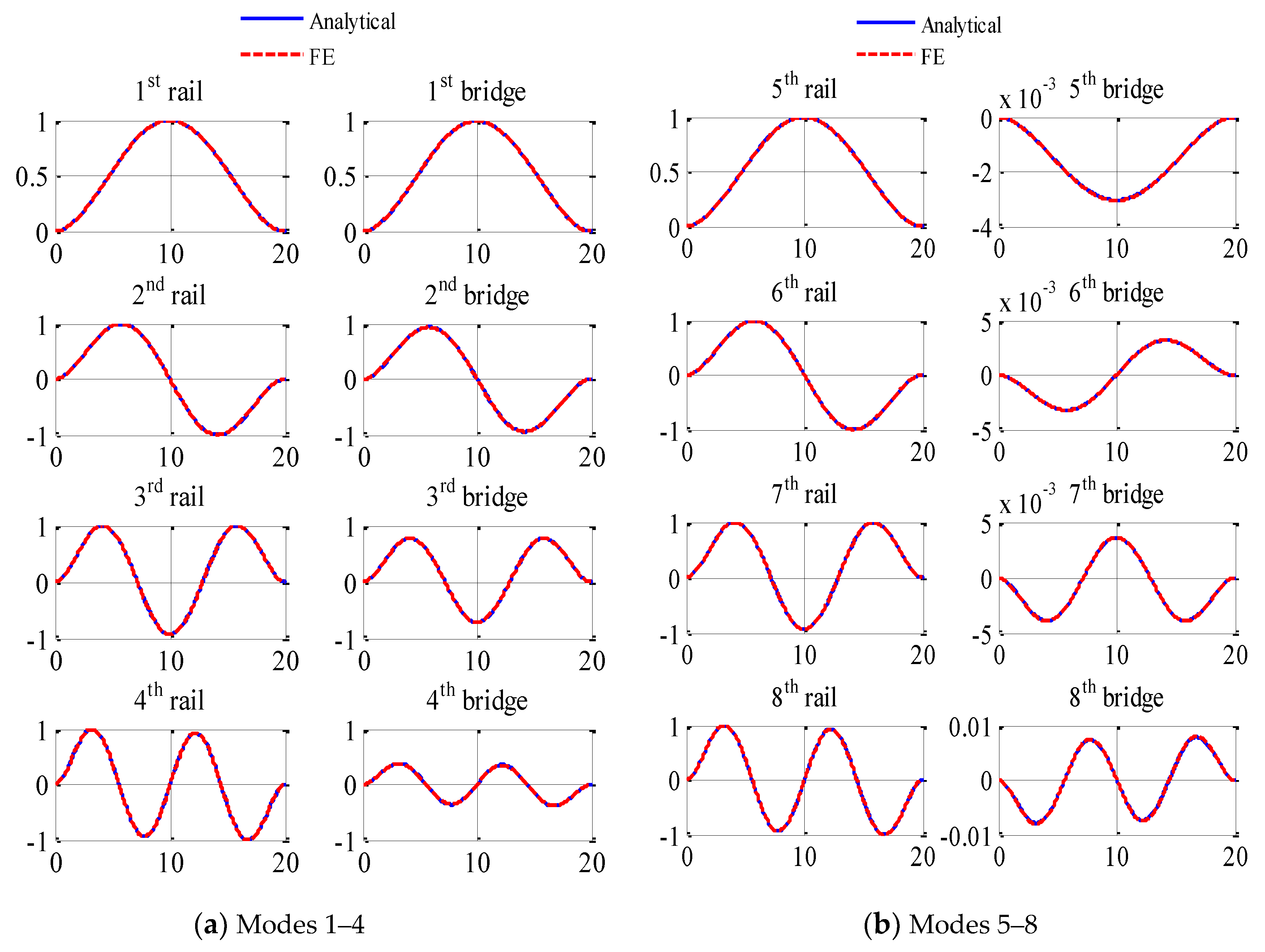
2.2. Verification of the Analytical Solutions in Section 2.1

To be concise, only the verifications for the frequencies and mode shapes of the fixed-fixed double-beam system are demonstrated in this section.

The material properties of the two beams are obtained from the rail and the bridge in the reference [2]. The properties of the bridge are: $I_{\mathrm{b}}=3.81{\mathrm{m}}^4$, ${\rho }_{\mathrm{b}}{A}_{\mathrm{b}}=34088\mathrm{kg}/\mathrm{m}$, $E_{\mathrm{b}}=2.943\times {10}^{10}\mathrm{Pa}$, $L_{\mathrm{b}}=20\mathrm{m}$. The properties of each rail are: $E_{\mathrm{r}}{I}_{\mathrm{r}}=4.3\times {10}^6{\mathrm{Nm}}^2$, ${\rho }_{\mathrm{r}}{A}_{\mathrm{r}}=51.5\mathrm{kg}/\mathrm{m}$. The length of each rail is set to be the same as the bridge. In the discrete spring model, the contact stiffness of each spring underlying one rail is $4.1125\times {10}^7\mathrm{N}/\mathrm{m}$ and the regular spacing between two neighboring contact springs is 0.625 m. In the distributed spring model, the contact stiffness under one rail is equivalent to be $4.1125\times {10}^7÷0.625=6.58\times {10}^7\mathrm{N}/{\mathrm{m}}^2$. In the 2D model, all the rail properties are doubled to account for the presence of both rails. The non-dimensional parameters are calculated to be: $s_{\mathrm{k}}=7.67\times {10}^{-5}$, $s_{\mathrm{m}}=0.003$ and $s_{\mathrm{e}}=0.0343$.

The discrete spring model for the rail-bridge system is established by the FE method and the numerical frequencies and mode shapes of the system are obtained. They are compared with the analytical counterparts calculated from the formulae for the distributed spring model in Section 2.1. The rail and the bridge are modeled by 256 beam elements in the FE model. 31 discrete spring elements having the stiffness of $8.225\times {10}^7$ N/m and the space of 0.625 m are created to model the discrete springs. The first 16 frequencies of the double-beam system are obtained by the FE method and compared with the analytical results as shown in

Table 4. Modal frequencies for the fixed-fixed double-beam system.

Mode Number	Frequency (Hz)		Difference
	FE	Analytical	(%)
1	16.12	16.12	0
2	44.44	44.44	0
3	87.08	87.08	0
4	143.66	143.68	0
5	179.90	180.72	0.5
6	180.03	180.85	0.5
7	180.49	181.31	0.5
8	181.77	182.59	0.5
9	182.20	183.01	0.4
10	185.72	186.57	0.5
11	190.52	191.38	0.5
12	197.36	198.23	0.4
13	206.69	207.61	0.4
14	216.22	216.24	0
15	218.82	219.77	0.4
16	233.99	234.96	0.4

. The differences between the two kinds of results are very small. To save page, only the first 8 mode shapes are depicted for comparison in Figure 2. The differences between the mode shapes obtained by the two methods cannot be distinguished. The above comparisons verify the analytical formulae in Section 2.1. It is interesting to find that the 5th mode shape is similar to the 1st except that the amplitude and direction of the bridge mode shape are different. The similarities can also be found between the 6th and the 2nd, the 7th and the 3rd and the 8th and the 4th mode shapes. In fact, the two similar modes are the two sub-modes corresponding to the same basic mode with the same wavenumber. The four sets of similar modes are corresponding to the first four basic modes. More studies about sub-modes are presented in Section 2.3.

2.3. Parametric Studies

To conduct the parametric study in the dimensionless form, the frequency ratios and mode shape amplitude ratios in two sub-modes are defined as follows

$${\omega }_{0,i}=\frac{{\omega }_n^{\left(i\right)}}{{\tilde{\omega }}_{2,n}}i=1,2$$

(47)

$${\varphi }_{0,i}=\frac{{\phi }_{1,n}^{\left(i\right)}}{{\phi }_{2,n}}i=1,2$$

(48)

The frequency ratios in Equation (47) and mode amplitude ratios in Equation (48) can be obtained analytically from Equations (9) and (22), respectively. The effects of the order of the basic mode (n), the contact stiffness ratio ($s_{\mathrm{e}}$), mass ratio ($s_{\mathrm{m}}$), stiffness ratio ($s_{\mathrm{k}}$) on the frequency ratios and the mode amplitude ratios in two sub-modes are investigated.

2.3.1. The Order of Basic Mode

Figure 3 shows the effect of the order of the basic mode (n) on the frequency ratios in two sub-modes (${\omega }_{0,i},i=1,2$) for different boundary conditions when $s_{\mathrm{e}}=100$, $s_{\mathrm{m}}=1$ and $s_{\mathrm{k}}=2$. It can be seen from the figure that ${\omega }_{0,1}$ and ${\omega }_{0,2}$ vary obviously with boundary conditions in the 1st basic mode. The effect of n on the frequency ratios is small when n is large. Figure 4 shows the effect of n on the mode amplitude ratios in two sub-modes $({\varphi }_{0,i,}i=1,2)$. ${\varphi }_{0,1}$ is always positive and ${\varphi }_{0,2}$ is always negative, which indicates that the modes of two beams are always in-plane with each other in the 1st sub-mode, whereas the modes of the primary beam are always anti-plane with the modes of the secondary beam in the 2nd sub-mode. ${\varphi }_{0,1}$ tends to be very small with the increase of n and ${\varphi }_{0,2}$ decreases dramatically after the 4th basic mode, which means that the double-beam system tends to behavior like two individual beams. While ${\varphi }_{0,1}$ varies a lot with boundary conditions in the 1st basic mode, ${\varphi }_{0,2}$ differs obviously with boundary conditions when n is larger than 5.

2.3.2. Contact Stiffness Ratio

The effect of the contact stiffness ratio ($s_{\mathrm{e}}$) on the frequency ratios (${\omega }_{0,i},i=1,2$) in the 1st basic mode for different boundary conditions when $s_{\mathrm{m}}=1$ and $s_{\mathrm{k}}=2$ is plotted in Figure 5. It can be seen from the figure that ${\omega }_{0,1}$ and ${\omega }_{0,2}$ increase monotonically with $s_{\mathrm{e}}$. ${\omega }_{0,1}$ increases dramatically when $s_{\mathrm{e}}$ is small. The increasing rates of ${\omega }_{0,1}$ and ${\omega }_{0,2}$ are larger for looser boundary conditions when $s_{\mathrm{e}}$ is smaller. Boundary conditions have a bigger influence on ${\omega }_{0,2}$ than ${\omega }_{0,1}$. Figure 6 shows that both ${\varphi }_{0,1}$ and ${\varphi }_{0,2}$ increase with $s_{\mathrm{e}}$ and the increasing rates of ${\varphi }_{0,1}$ and ${\varphi }_{0,2}$ are very large when $s_{\mathrm{e}}$. is small. In addition, the increasing rates of ${\varphi }_{0,1}$ and ${\varphi }_{0,2}$ are larger for looser boundary conditions when $s_{\mathrm{e}}$ is smaller.

2.3.3. Mass Ratio

The effect of the mass ratio ($s_{\mathrm{m}}$) on the frequency ratios (${\omega }_{0,i},i=1,2$) in the 1st basic mode for different boundary conditions is depicted in Figure 7. Both ${\omega }_{0,1}$ and ${\omega }_{0,2}$ decrease with $s_{\mathrm{m}}$ and the decreasing rate of ${\omega }_{0,2}$ is very large when $s_{\mathrm{m}}$ is small. Figure 8 shows the effect of $s_{\mathrm{m}}$ on the mode amplitude ratios (${\varphi }_{0,i},i=1,2$) in the 1st basic mode for different boundary conditions. Both ${\varphi }_{0,1}$ and ${\varphi }_{0,2}$ increase with $s_{\mathrm{m}}$ and the increasing rates are large when $s_{\mathrm{m}}$ is small. ${\varphi }_{0,1}$ is smaller than 1 when $s_{\mathrm{m}}$ is smaller than 1 and ${\varphi }_{0,1}$ is larger than 1 when $s_{\mathrm{m}}$ is larger than 1. ${\varphi }_{0,2}$ is smaller than −1 when $s_{\mathrm{m}}$ is smaller than 1 and ${\varphi }_{0,2}$ is larger than −1 when $s_{\mathrm{m}}$ is larger than 1. ${\varphi }_{0,1}$ and ${\varphi }_{0,2}$ are closer to 1 for looser boundary conditions, which means that the modes of two beams are closer to each other for looser boundary conditions.

2.3.4. Beam Stiffness Ratio

The effect of the beam stiffness ratio ($s_{\mathrm{k}}$) on the frequency ratios (${\omega }_{0,i},i=1,2$) in the 1st basic mode for different boundary conditions is shown in Figure 9. Both ${\omega }_{0,1}$ and ${\omega }_{0,2}$ increase with $s_{\mathrm{k}}$. The influence of boundary conditions on ${\omega }_{0,1}$ is big when $s_{\mathrm{k}}$ is large. Figure 10 shows the effect of $s_{\mathrm{k}}$ on the mode amplitude ratios (${\varphi }_{0,i},i=1,2$) for different boundary conditions in the 1st basic mode. Both ${\varphi }_{0,1}$ and ${\varphi }_{0,2}$ decrease with $s_{\mathrm{m}}$ and the decreasing rates are large when $s_{\mathrm{m}}$ is small. ${\varphi }_{0,1}$ is larger than 1 when $s_{\mathrm{m}}$ is smaller than 1 and ${\varphi }_{0,1}$ is smaller than 1 when $s_{\mathrm{m}}$ is larger than 1. ${\varphi }_{0,2}$ is larger than −1 when $s_{\mathrm{m}}$ is smaller than 1 and ${\varphi }_{0,2}$ is smaller than −1 when $s_{\mathrm{m}}$ is larger than 1. ${\varphi }_{0,1}$ and ${\varphi }_{0,2}$ are closer to 1 for looser boundary conditions, which means that the modes of two beams are closer to each other for looser boundary conditions.

3. Double-Beam System Traversed by a Moving Force

The vibrations of the double-beam system with five general kinds of symmetric boundary conditions subjected to a moving force are studied in this section. The force is considered to move at a constant speed of $v$ on the primary beam, as shown in Figure 11.

3.1. Mathematical Formulation

The equations of motion of the secondary beam and the primary beam can be expressed as

$$E_2{I}_2{w}_2^{⁗}+{\rho }_2{A}_2{\ddot{w}}_2-k_{\mathrm{e}}\left(w_1-w_2\right)=0$$

(49)

$$s_{\mathrm{k}}{E}_2{I}_2{w}_1^{⁗}+s_{\mathrm{m}}{\rho }_2{A}_2{\ddot{w}}_1+k_{\mathrm{e}}\left(w_1-w_2\right)=-f\delta \left(x-vt\right)$$

(50)

The sum of Equations (49) and (50) is

$$E_2{I}_2(s_{\mathrm{k}}{w}_1^{⁗}+w_2^{⁗})+{\rho }_2{A}_2\left(s_{\mathrm{m}}{\ddot{w}}_1+{\ddot{w}}_2\right)=-f\delta \left(x-vt\right)$$

(51)

Applying the MS method to Equation (51), one can obtain the following ordinary differential equation regarding modal coordinates [42,43]

$${\ddot{q}}_n^{\left(i\right)}\left(t\right)+{\left({\omega }_n^{\left(i\right)}\right)}^2{q}_n^{\left(i\right)}\left(t\right)=-\frac{f{\phi }_{1,n}^{\left(i\right)}\left(vt\right)}{M_{nn}^{\left(i\right)}},n=1,2,3\dots ,i=1,2$$

(52)

where

$$M_{nn}^{\left(i\right)}={{\displaystyle \int }}_0^l{s}_{\mathrm{m}}{\rho }_2{A}_2{\left[{\phi }_{1,n}^{\left(i\right)}\left(x\right)\right]}^2\mathrm{d}x+{{\displaystyle \int }}_0^l{\rho }_2{A}_2{\left[{\phi }_{2,n}\left(x\right)\right]}^2\mathrm{d}x$$

(53)

3.1.1. Fixed-Fixed and Fixed-Pinned Boundary Conditions

It is found in Section 2.1 that the mode shapes of the double beam system for fixed-fixed boundary conditions have the same mathematical formulae as those for fixed-pinned boundary conditions except that the values of $r_{1}l$ are different, so the solutions of Equation (52) would have the same formulae for the two kinds of boundary conditions except the values of $r_{1}l$. The following derivations are based on double-beam systems with fixed-fixed boundary conditions.

Substituting Equations (21) and (22) into Equation (53) and setting C to be one result in

$$M_{nn}^{\left(i\right)}={\rho }_2{A}_{2}l\left[1+s_{\mathrm{m}}{\left(A_n^{\left(i\right)}\right)}^2\right]$$

(54)

where

$$A_n^{\left(i\right)}=1+\frac{1-{\left(\frac{{\omega }_n^{\left(i\right)}}{{\tilde{\omega }}_{2,n}}\right)}^2}{s_e}{\left(r_1^{\left(n\right)}l\right)}^4$$

(55)

and ${\omega }_n^{\left(i\right)}$ and ${\tilde{\omega }}_{2,n}$ are obtained from Equations (9) and (11), respectively.

Substituting Equation (22) into Equation (52) and setting C to be one result in

$${\ddot{q}}_n^{\left(i\right)}+{\left({\omega }_n^{\left(i\right)}\right)}^2{q}_n^{\left(i\right)}=-\frac{f{A}_n^{\left(i\right)}}{M_{nn}^{\left(i\right)}}\left[\cos \left(r_1^{\left(n\right)}vt\right)-\cosh \left(r_1^{\left(n\right)}vt\right)-B_n\left(\sin \left(r_1^{\left(n\right)}vt\right)-\sinh \left(r_1^{\left(n\right)}vt\right)\right)\right]$$

(56)

where

$$B_n=\frac{\cos (r_1^{\left(n\right)}l)-\cosh (r_1^{\left(n\right)}l)}{\sin (r_1^{\left(n\right)}l)-\sinh (r_1^{\left(n\right)}l)}$$

(57)

The solution of Equation (56) is

$$q_n^{\left(i\right)}=p_n^{\left(i\right)}\left(\frac{\cos \left(r_1^{\left(n\right)}vt\right)-B_n\sin \left(r_1^{\left(n\right)}vt\right)}{1-{\left(s_n^{\left(i\right)}\right)}^2}-\frac{\cosh \left(r_1^{\left(n\right)}vt\right)-B_n\sinh \left(r_1^{\left(n\right)}vt\right)}{1+{\left(s_n^{\left(i\right)}\right)}^2}-\frac{2{\left(s_n^{\left(i\right)}\right)}^2\left[\cos \left({\omega }_n^{\left(i\right)}t\right)-B_n{s}_n^{\left(i\right)}\sin \left({\omega }_n^{\left(i\right)}t\right)\right]}{\left[1-{\left(s_n^{\left(i\right)}\right)}^2\right]\left[1+{\left(s_n^{\left(i\right)}\right)}^2\right]}\right)$$

(58)

where

$$\{\begin{array}{c}{s}_n^{\left(i\right)}=\frac{r_1^{\left(n\right)}v}{{\omega }_n^{\left(i\right)}}\\ p_n^{\left(i\right)}=-\frac{f{A}_n^{\left(i\right)}}{M_{nn}^{\left(i\right)}{\left({\omega }_n^{\left(i\right)}\right)}^2}\end{array}$$

(59)

The displacements of the primary beam and the secondary beam are

$$w_1\left(x,t\right)={\displaystyle \sum }_{n=1}^m\left[{\phi }_{1,n}^{\left(1\right)}{q}_n^{\left(1\right)}\left(t\right)+{\phi }_{1,n}^{\left(2\right)}{q}_n^{\left(2\right)}\left(t\right)\right]$$

(60)

$$w_2\left(x,t\right)={\displaystyle \sum }_{n=1}^m{\phi }_{2,n}\left(x\right)\left[q_n^{\left(1\right)}\left(t\right)+q_n^{\left(2\right)}\left(t\right)\right]$$

(61)

where m is the number of basic modes used in the MS method.

To conduct parametric studies in Section 3.3, two dimensionless displacements for the primary beam and the secondary beam are defined as follows

$${\overline{w}}_i=\frac{w_i\left(x_{\max },\overline{t}\right)}{w_s},i=1,2$$

(62)

where $x_{\max }$ represents the location where maximum static deflection takes place; $w_s$ is the maximum static deflection of a single secondary beam with the same boundary conditions as the double-beam loaded by a concentrated force $f$ at $x_{\max }$ of the single beam and $\overline{t}$ is a dimensionless time

$$\overline{t}=\frac{vt}{l}$$

(63)

For a fixed-fixed beam, $x_{\max }=0.5l$ and $w_s$ is

$$w_s=-\frac{f{L}^3}{192E_2{I}_2}$$

(64)

For a fixed-pinned beam, $x_{\max }=0.55l$ and w_s is

$$w_s=-\frac{f{L}^3}{48\sqrt{5}{E}_2{I}_2}$$

(65)

The speed ratio is defined as

$$\alpha =\frac{v}{v_{cr}}$$

(66)

where $v_{cr}$ is the critical speed at which the single secondary beam is excited into resonance in the first mode by the moving force

$$v_{cr}=\frac{{\tilde{\omega }}_{2,1}L}{\pi }$$

(67)

and the first frequency of the single secondary beam ${\tilde{\omega }}_{2,1}$ can be obtained by

$${\tilde{\omega }}_{2,1}={\left(r_1^{\left(1\right)}\right)}^2\sqrt{\frac{E_2{I}_2}{{\rho }_2{A}_2}}$$

(68)

3.1.2. Pinned-Pinned Boundary Conditions

Substituting Equations (28) and (29) into Equation (53) and setting C to be one result in

$$M_{nn}^{\left(i\right)}=\frac{1}{2}{\rho }_2{A}_{2}l\left[1+s_{\mathrm{m}}{\left(A_n^{\left(i\right)}\right)}^2\right]$$

(69)

where

$$A_n^{\left(i\right)}=1+\frac{1-{\left(\frac{{\omega }_n^{\left(i\right)}}{{\tilde{\omega }}_{2,n}}\right)}^2}{s_e}{\left(n\pi \right)}^4$$

(70)

and ${\omega }_n^{\left(i\right)}$ and ${\tilde{\omega }}_{2,n}$ are obtained from Equations (9) and (30), respectively.

Substituting Equation (29) into Equation (52) and setting C to be one result in

$${\ddot{q}}_n^{\left(i\right)}+{\left({\omega }_n^{\left(i\right)}\right)}^2{q}_n^{\left(i\right)}=-\frac{f{A}_n^{\left(i\right)}}{M_{nn}^{\left(i\right)}}\sin \left(\frac{n\pi v}{l}t\right)$$

(71)

It is noticed that Equation (71) has the same form as that of a pinned-pinned single beam excited by a moving force. The solution of Equation (71) is

$$q_n^{\left(i\right)}\left(t\right)=\frac{p_n^{\left(i\right)}}{1-{\left(s_n^{\left(i\right)}\right)}^2}\left[\sin \left(\frac{n\pi v}{l}t\right)-s_n^{\left(i\right)}\sin \left({\omega }_n^{\left(i\right)}t\right)\right]$$

(72)

where $p_n^{\left(i\right)}$ is the same expression as that in Equation (59) and $s_n^{\left(i\right)}$ is

$$s_n^{\left(i\right)}=\frac{n\pi v}{l{\omega }_n^{\left(i\right)}}$$

(73)

The displacements of the primary beam and the secondary beam are

$$w_1\left(x,t\right)={\displaystyle \sum }_{n=1}^m\sin \left(\frac{n\pi }{l}x\right)\left[A_n^{\left(1\right)}{q}_n^{\left(1\right)}\left(t\right)+A_n^{\left(2\right)}{q}_n^{\left(2\right)}\left(t\right)\right]$$

(74)

$$w_2\left(x,t\right)={\displaystyle \sum }_{n=1}^m\sin \left(\frac{n\pi }{l}x\right)\left[q_n^{\left(1\right)}\left(t\right)+q_n^{\left(2\right)}\left(t\right)\right]$$

(75)

For a pinned-pinned beam, $x_{\max }=0.5l$ and $w_s$ becomes

$$w_s=-\frac{f{L}^3}{48E_2{I}_2}$$

(76)

3.1.3. Pinned-Fixed Boundary Conditions

Substituting Equations (40) and (22) into Equation (53) and setting C to be one result in

$$M_{nn}^{\left(i\right)}=\frac{1}{2}{\rho }_2{A}_{2}l\left[1+s_{\mathrm{m}}{\left(A_n^{\left(i\right)}\right)}^2\right]$$

(77)

where $A_n^{\left(i\right)}$ has the same form as Equation (55).

Substituting Equation (22) into Equation (52) and setting C to be one result in

$${\ddot{q}}_n^{\left(i\right)}+{\left({\omega }_n^{\left(i\right)}\right)}^2{q}_n^{\left(i\right)}=-\frac{f{A}_n^{\left(i\right)}}{M_{nn}^{\left(i\right)}}[\sin (r_1^{\left(n\right)}vt)-\frac{\sin r_1^{\left(n\right)}l}{\sinh r_1^{\left(n\right)}l}\sinh (r_1^{\left(n\right)}vt)]$$

(78)

The solution of Equation (78) is

$$q_n^{(i)}\left(t\right)=p_n^{(i)}\left[\frac{\sin \left(r_1^{(n)}vt\right)}{1-{\left(s_n^{(i)}\right)}^2}-\frac{\sin r_1^{(n)}l}{\sinh r_1^{(n)}l}\frac{\sinh \left(r_1^{(n)}vt\right)}{1+{\left(s_n^{(i)}\right)}^2}+(\frac{\sin r_1^{(n)}l}{\sinh r_1^{(n)}{l}_1}\frac{s_n^{(i)}}{1+{\left(s_n^{(i)}\right)}^2}-\frac{s_n^{(i)}}{1-{\left(s_n^{(i)}\right)}^2})\sin \left({\omega }_n^{(i)}t\right)\right]$$

(79)

where $p_n^{\left(i\right)}$ and $s_n^{\left(i\right)}$ have the same form as Equation (59).

The displacements of the double beam systems can be worked by Equations (60) and (61).

For a pinned-fixed beam, $x_{\max }=0.45l$ and $w_s$ is

$$w_s=-\frac{f{L}^3}{48\sqrt{5}{E}_2{I}_2}$$

(80)

3.1.4. Fixed-Free Boundary Conditions

Substituting Equations (46) and (22) into Equation (53) and setting C to be one result in the same formula as Equation (54). It is found in Section 2.1 that the mode shapes of the fixed-free double-beam systems have similar formulae as those for fixed-fixed double-beam systems. The solution to Equation (52) for fixed-free double beam systems is the same as Equation (58) except

$$B_n=\frac{\cos (r_1^{\left(n\right)}l)+\cosh (r_1^{\left(n\right)}l)}{\sin (r_1^{\left(n\right)}l)+\sinh (r_1^{\left(n\right)}l)}$$

(81)

For a fixed-free beam, $x_{\max }=l$ and $w_s$ becomes

$$w_s=-\frac{f{L}^3}{3E_2{I}_2}$$

(82)

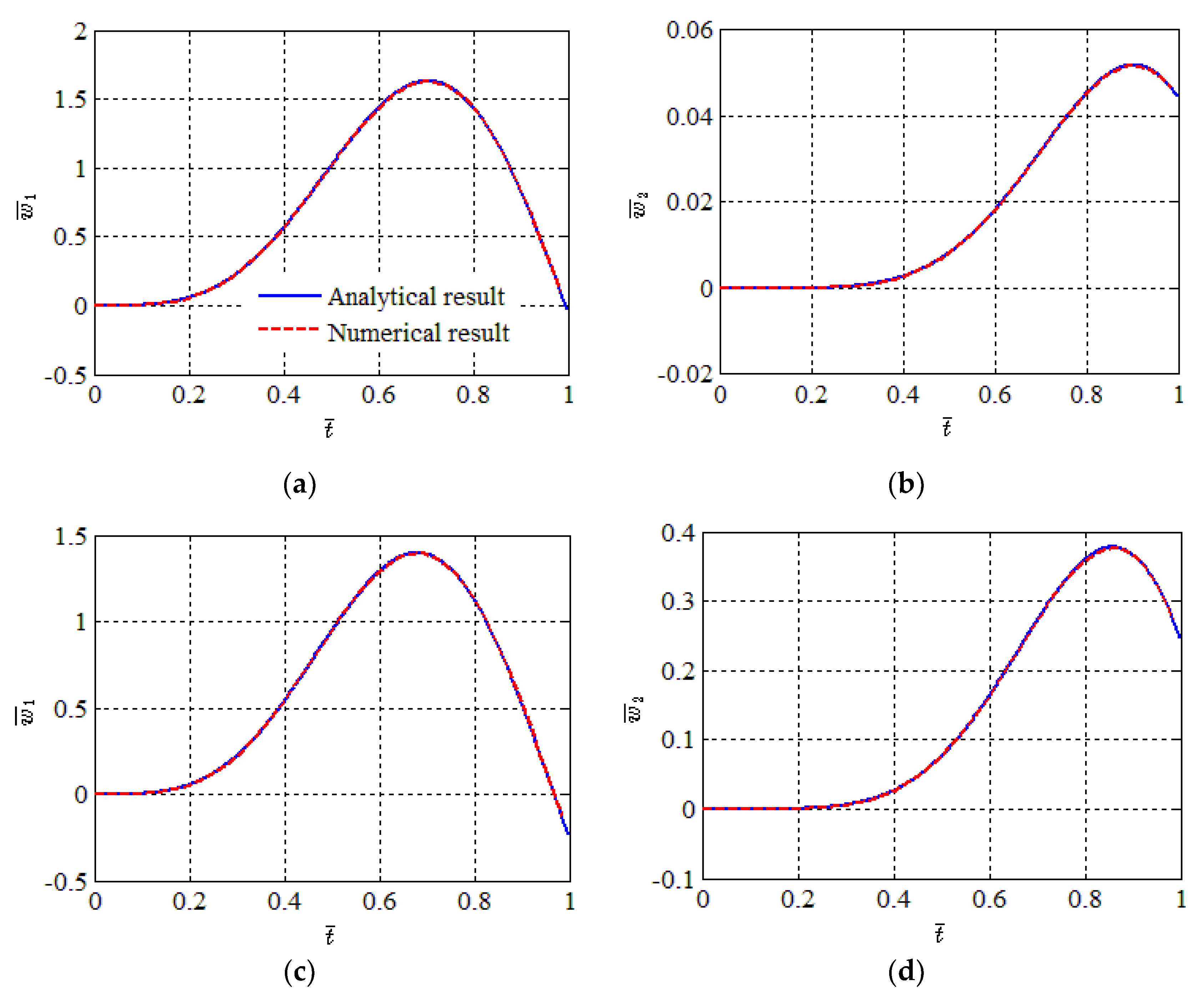
3.2. Verification of the Analytical Solutions in Section 3.1

An example of the double-beam system with two identical beams ($s_{\mathrm{m}}=1,s_{\mathrm{k}}=1$) subjected to a moving force is used firstly to verify the analytical solutions in Section 3.1. To be concise, only the formulae for fixed-fixed and pinned-pinned boundary conditions are verified.

3.2.1. Fixed-Fixed Boundary Conditions

The Newmark-Beta integration method is adopted to obtain numerical solutions of Equation (52) and compared with its analytical solutions. It is found in computations that using only the first basic mode (m = 1) is good enough to reach satisfied accuracies for the fixed-fixed double-beam system. For comparison, only the first basic mode is used in the following analyses for other kinds of boundary conditions. Figure 12 shows the comparisons between the results by the two methods for the dimensionless speed ($\mathsf{\alpha }$) of 0.5 and contact stiffness ratios ($s_{\mathrm{e}}$) of 10 and 100. It can be seen from the figure that the two kinds of results have very good agreements. In addition, it can be found that the maximum displacement of the secondary beam (${\overline{w}}_{2,\max }$) is smaller than that of the primary beam (${\overline{w}}_{1,\max }$) and the instants for ${\overline{w}}_{2,\max }$ lag behind those for ${\overline{w}}_{1,\max }$. When $s_{\mathrm{e}}$ becomes larger, the difference between ${\overline{w}}_{1,\max }$ and ${\overline{w}}_{2,\max }$ is smaller.

3.2.2. Pinned-Pinned Boundary Conditions

The obtained analytical results by MS method are compared with those by the Equation Decoupled (ED) method in Reference [19]. Figure 13 shows the comparisons between the results by the two methods for the dimensionless speed (α) of 0.5 and contact stiffness ratio ($s_{\mathrm{e}}$) of 10 and 100. The two groups of results agree with each other very well. It can also be seen from the figure that the difference between ${\overline{w}}_{1,\max }$ and ${\overline{w}}_{2,\max }$ becomes smaller with the increase of $s_{\mathrm{e}}$. More detailed study about the relationship between ${\overline{w}}_{i,\max }\left(i=1,2\right)$ and $s_{\mathrm{e}}$ will be shown in Section 3.3.

3.3. Parametric Studies

The dimensionless displacements of the primary beam (${\overline{w}}_1$) and the secondary beam (${\overline{w}}_2$) are affected by four dimensionless parameters: speed ratio ($\alpha$), contact stiffness ratio ($s_{\mathrm{e}}$), mass ratio (${\mathrm{s}}_{\mathrm{m}}$) and beam stiffness ratio (${\mathrm{s}}_{\mathrm{k}}$). The effects of these parameters on the maximum dimensionless displacements of the primary beam (${\overline{w}}_{1,\max }$) and the secondary beam (${\overline{w}}_{2,\max }$) are investigated for five kinds of boundary conditions.

3.3.1. Speed Ratio

Figure 14 shows the maximum dimensionless displacements of the primary beam (${\overline{w}}_{1,\max }$) and the secondary beam (${\overline{w}}_{2,\max }$) versus the speed ratio ($\alpha$) for different boundary conditions ($s_{\mathrm{e}}$) when $s_{\mathrm{e}}=100$, $s_{\mathrm{m}}=1$ and $s_{\mathrm{k}}=1$. It can be found from the figure that the difference between ${\overline{w}}_{1,\max }$ and ${\overline{w}}_{2,\max }$ is smaller for looser boundary conditions.

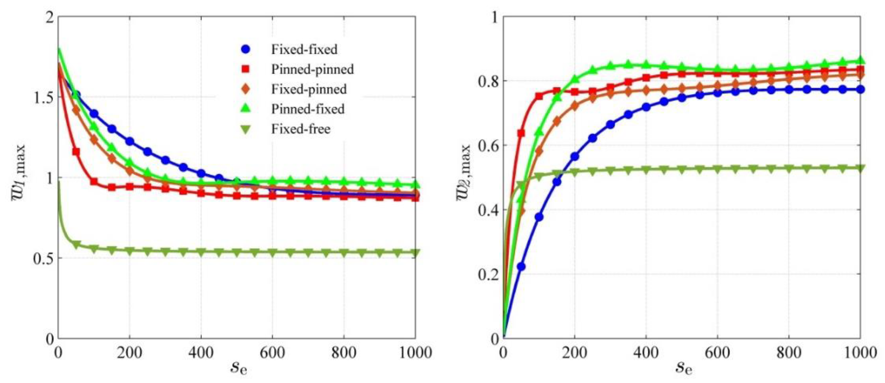
3.3.2. Contact Stiffness Ratio

Figure 15 shows maximum dimensionless displacements (${\overline{w}}_{1,\max }$) and (${\overline{w}}_{2,\max }$) versus the contact stiffness ratio ($s_{\mathrm{e}}$) for different boundary conditions when $\alpha =0.5$, $s_{\mathrm{m}}=1$ and $s_{\mathrm{k}}=1$. Several characteristics can be found from the figure:

• ${\overline{w}}_{1,\max }$ generally decreases with $s_{\mathrm{e}}$ and the opposite trend is true for ${\overline{w}}_{2,\max }$;
• The varying rates of ${\overline{w}}_{i,\max }\left(i=1,2\right)$ are very large when $s_{\mathrm{e}}$ is below a turning point and become much smaller when $s_{\mathrm{e}}$ is beyond the turning point;
• With the increase of $s_{\mathrm{e}}$, ${\overline{w}}_{1,\max }$ and ${\overline{w}}_{2,\max }$ tend to be the same value which is half of that for a single beam with the same boundary conditions and at the same values of $\alpha$, $s_{\mathrm{m}}$ and $s_{\mathrm{k}}$;
• The difference between ${\overline{w}}_{1,\max }$ and ${\overline{w}}_{2,\max }$ is generally smaller for looser boundary conditions.

3.3.3. Mass Ratio

Figure 16 shows maximum dimensionless displacements (${\overline{w}}_{1,\max }$) and (${\overline{w}}_{2,\max }$) versus the mass ratio ($s_{\mathrm{m}}$) for different boundary conditions when $\mathsf{\alpha }=0.5$, $s_{\mathrm{e}}=50$ and $s_{\mathrm{k}}=1$. It can be seen from the figure that ${\overline{w}}_{i,\max }\left(i=1,2\right)$ increases firstly and then decreases with $s_{\mathrm{m}}$. In addition, the difference between ${\overline{w}}_{1,\max }$ and ${\overline{w}}_{2,\max }$ is smaller for looser boundary conditions.

3.3.4. Beam Stiffness Ratio

Figure 17 shows maximum dimensionless displacements (${\overline{w}}_{1,\max }$) and (${\overline{w}}_{2,\max }$) versus the beam stiffness ratio ($s_{\mathrm{k}}$) for different boundary conditions when $\alpha =0.5$, $s_{\mathrm{e}}=50$ and $s_{\mathrm{m}}=1$. It can be seen from the figure that both ${\overline{w}}_{1,\max }$ and ${\overline{w}}_{2,\max }$ decrease with $s_{\mathrm{k}}$ and the decreasing rate is large when $s_{\mathrm{k}}$ is small. The influence of boundary conditions on ${\overline{w}}_{i,\max }\left(i=1,2\right)$ is basically bigger when $s_{\mathrm{k}}$ is smaller.

4. Conclusions

The vibrations of the double-beam system with five general kinds of symmetric boundary conditions traversed by a moving force are studied analytically by using the Modal Superposition (MS) method in this paper. Main conclusions can be drawn as below:

(1)

Each wavenumber corresponds to two sub-modes of the system. The mode shapes of one beam of the system are the same as those for the single beam with the same boundary condition. The amplitudes of the mode shapes for one beam of the double-beam system are the multiple of those for the other beam of the system.

(2)

The two sub-modes corresponding to the first wavenumber both make significant contributions to the dynamics of the system under a moving load, which is different from the case for a single beam.

(3)

The maximum dynamic displacement of the primary beam generally decreases with the stiffness of the contact springs. The opposite trend is true for the maximum dynamic displacement of the secondary beam. The two beams vibrate together when the contact springs are very stiff. With the increase of the ratio between the mass of the primary beam and the secondary beam, the maximum dynamic displacement ratios of both beams increases first and then decreases. The maximum dynamic displacement ratios of both beams are smaller for a larger bending stiffness ratio of the primary beam to the secondary beam.

(4)

The primary beam tends to vibrate together with the secondary beam when the boundary condition of the system is looser.

References

1. Hussein, M.F.M.; Hunt, H.E.M. Modelling of floating-slab tracks with continuous slabs under oscillating moving loads. J. Sound Vib. 2006, 297, 37–54. [Google Scholar] [CrossRef]
2. Cheng, Y.S.; Au, F.T.K.; Cheung, Y.K. Vibration of railway bridges under a moving train by using bridge-track-vehicle element. Eng. Struct. 2001, 23, 1597–1606. [Google Scholar] [CrossRef]
3. Lou, P. Finite element analysis for train–track–bridge interaction system. Arch. Appl. Mech. 2007, 77, 707–728. [Google Scholar] [CrossRef]
4. Galuppi, L.; Royer-Carfagni, G. Laminated beams with viscoelastic interlayer. Int. J. Solids Struct. 2012, 49, 2637–2645. [Google Scholar] [CrossRef]
5. Hamada, T.R.; Nakayama, H.; Hayashi, K. Free and forced vibrations of elastically connected double-beam systems. Bull. JSME 1983, 26, 1936–1942. [Google Scholar] [CrossRef]
6. Chen, Y.H.; Sheu, J.T. Dynamic characteristics of layered beam with flexible core. J. Vib. Acoust. 1994, 116, 350–356. [Google Scholar] [CrossRef]
7. Rahmani, O.; Norouzi, S.; Golmohammadi, H.; Hosseini, S.A.H. Dynamic response of a double, single-walled carbon nanotube under a moving nanoparticle based on modified nonlocal elasticity theory considering surface effects. Mech. Adv. Mater. Struct. 2017, 24, 1274–1291. [Google Scholar] [CrossRef]
8. Seelig, J.M.; Hoppmann, W.H., II. Normal mode vibrations of systems of elastically connected parallel bars. J. Acoust. Soc. Am. 1964, 36, 93–99. [Google Scholar] [CrossRef]
9. Rao, S.S. Natural vibrations of systems of elastically connected Timoshenko beams. J. Acoust. Soc. Am. 1974, 55, 1232–1237. [Google Scholar] [CrossRef]
10. Oniszczuk, Z. Free Transverse Vibrations Of Elastically Connected Simply Supported Double-Beam Complex System. J. Sound Vib. 2000, 232, 387–403. [Google Scholar] [CrossRef]
11. Mirzabeigy, A.; Dabbagh, V.; Madoliat, R. Explicit formulation for natural frequencies of double-beam system with arbitrary boundary conditions. J. Mech. Sci. Technol. 2017, 31, 515–521. [Google Scholar] [CrossRef]
12. Han, F.; Dan, D.; Cheng, W. An exact solution for dynamic analysis of a complex double-beam system. Compos. Struct. 2018, 193, 295–305. [Google Scholar] [CrossRef]
13. Hao, Q.; Zhai, W.; Chen, Z. Free vibration of connected double-beam system with general boundary conditions by a modified Fourier–Ritz method. Arch. Appl. Mech. 2018, 88, 741–754. [Google Scholar] [CrossRef]
14. Xiang, P.; Zhao, Y.; Lin, J.; Kennedy, D.; Williams, F.W. Random vibration analysis for coupled vehicle-track systems with uncertain parameters. Eng. Comput. 2016, 33, 443–464. [Google Scholar] [CrossRef]
15. Kordestani, H.; Xiang, Y.-Q.; Ye, X.-W.; Jia, Y.-K. Application of the Random Decrement Technique in Damage Detection under Moving Load. Appl. Sci. 2018, 8, 753. [Google Scholar] [CrossRef]
16. Wang, W.; Deng, L.; Shao, X. Number of stress cycles for fatigue design of simply-supported steel I-girder bridges considering the dynamic effect of vehicle loading. Eng. Struct. 2016, 110, 70–78. [Google Scholar] [CrossRef]
17. Chen, Y.; Zhang, B.; Zhang, N.; Zheng, M. A Condensation Method for the Dynamic Analysis of Vertical Vehicle–Track Interaction Considering Vehicle Flexibility. J. Vib. Acoust. 2015, 137, 041010. [Google Scholar] [CrossRef]
18. Vu, H.V.; OrdÓÑEz, A.M.; Karnopp, B.H. Vibration of a Double-Beam System. J. Sound Vib. 2000, 229, 807–822. [Google Scholar] [CrossRef]
19. Abu-Hilal, M. Dynamic response of a double Euler–Bernoulli beam due to a moving constant load. J. Sound Vib. 2006, 297, 477–491. [Google Scholar] [CrossRef]
20. Wu, Y.; Gao, Y. Analytical Solutions for Simply Supported Viscously Damped Double-Beam System under Moving Harmonic Loads. J. Eng. Mech. 2015, 141, 04015004. [Google Scholar] [CrossRef]
21. Wu, Y.; Gao, Y. Dynamic response of a simply supported viscously damped double-beam system under the moving oscillator. J. Sound Vib. 2016, 384, 194–209. [Google Scholar] [CrossRef]
22. Zhang, Y.Q.; Lu, Y.; Ma, G.W. Effect of compressive axial load on forced transverse vibrations of a double-beam system. Int. J. Mech. Sci. 2008, 50, 299–305. [Google Scholar] [CrossRef]
23. Kessel, P.G. Resonances Excited in an Elastically Connected Double-Beam System by a Cyclic Moving Load. J. Acoust. Soc. Am. 1966, 40, 684–687. [Google Scholar] [CrossRef]
24. Kessel, P.G.; Raske, T.F. Damped Response of an Elastically Connected Double-Beam System Due to a Cyclic Moving Load. J. Acoust. Soc. Am. 1967, 42, 873–881. [Google Scholar] [CrossRef]
25. Oniszczuk, Z. Forced transverse vibrations of an elastically connected complex simply supported double-beam system. J. Sound Vib. 2003, 264, 273–286. [Google Scholar] [CrossRef]
26. Chonan, S. Dynamical behaviors of elastically connected double-beam systems subjected to an impulsive load. Bull. JSME 1976, 19, 595–603. [Google Scholar] [CrossRef]
27. Pavlović, R.; Kozić, P.; Pavlović, I. Dynamic stability and instability of a double-beam system subjected to random forces. Int. J. Mech. Sci. 2012, 62, 111–119. [Google Scholar] [CrossRef]
28. Stojanović, V.; Kozić, P. Forced transverse vibration of Rayleigh and Timoshenko double-beam system with effect of compressive axial load. Int. J. Mech. Sci. 2012, 60, 59–71. [Google Scholar] [CrossRef]
29. Kozić, P.; Pavlović, R.; Karličić, D. The flexural vibration and buckling of the elastically connected parallel-beams with a Kerr-type layer in between. Mech. Res. Commun. 2014, 56, 83–89. [Google Scholar] [CrossRef]
30. Kukla, S.; Skalmierski, B. Free vibration of a system composed of two beams separated by an elastic layer. J. Theor. Appl. Mech. 1994, 3, 581–590. [Google Scholar]
31. Mao, Q.; Wattanasakulpong, N. Vibration and stability of a double-beam system interconnected by an elastic foundation under conservative and nonconservative axial forces. Int. J. Mech. Sci. 2015, 93, 1–7. [Google Scholar] [CrossRef]
32. Li, Y.X.; Sun, L.Z. Transverse vibration of undamped elastically connected double-beam system with arbitrary boundary conditions. J. Eng. Mech. 2016, 142, 04015070. [Google Scholar] [CrossRef]
33. Li, Y.X.; Hu, Z.J.; Sun, L.Z. Dynamical behavior of a double-beam system interconnected by a viscoelastic layer. Int. J. Mech. Sci. 2016, 105, 291–303. [Google Scholar] [CrossRef]
34. Şimşek, M.; Cansız, S. Dynamics of elastically connected double-functionally graded beam systems with different boundary conditions under action of a moving harmonic load. Compos. Struct. 2012, 94, 2861–2878. [Google Scholar] [CrossRef]
35. Zhang, Z.; Huang, X.; Zhang, Z.; Hua, H. On the transverse vibration of Timoshenko double-beam systems coupled with various discontinuities. Int. J. Mech. Sci. 2014, 89, 222–241. [Google Scholar] [CrossRef]
36. Chen, Y.H.; Sheu, J.T. Beam on viscoelastic foundation and layered beam. J. Eng. Mech. 1995, 121, 340–344. [Google Scholar] [CrossRef]
37. Li, J.; Hua, H. Spectral finite element analysis of elastically connected double-beam systems. Finite Elem. Anal. Des. 2007, 43, 1155–1168. [Google Scholar] [CrossRef]
38. Palmeri, A.; Adhikari, S. A Galerkin-type state-space approach for transverse vibrations of slender double-beam systems with viscoelastic inner layer. J. Sound Vib. 2011, 330, 6372–6386. [Google Scholar] [CrossRef]
39. Jun, L.; Hongxing, H.; Xiaobin, L. Dynamic stiffness matrix of an axially loaded slender double-beam element. Struct. Eng. Mech. 2010, 35, 717–733. [Google Scholar] [CrossRef]
40. Lou, P. A vehicle-track-bridge interaction element considering vehicle’s pitching effect. Finite Elem. Anal. Des. 2005, 41, 397–427. [Google Scholar] [CrossRef]
41. Jing, H.; He, X.; Zou, Y.; Wang, H. In-plane modal frequencies and mode shapes of two stay cables interconnected by uniformly distributed cross-ties. J. Sound Vib. 2018, 417, 38–55. [Google Scholar] [CrossRef]
42. Yang, J.; Ouyang, H.; Stǎncioiu, D. Numerical studies of vibration of four-span continuous plate with rails excited by moving car with experimental validation. Int. J. Struct. Stab. Dyn. 2017, 17, 2039–2060. [Google Scholar] [CrossRef]
43. Yang, J.; Ouyang, H.; Stǎncioiu, D. An approach of solving moving load problems by Abaqus and Matlab using numerical modes. In Proceedings of the 7th International Conference on Vibration Engineering, Shanghai, China, 18–20 September 2015. [Google Scholar]
Figure 1. Double-beam system with symmetric boundary conditions.
Applsci 09 01218 g001
Figure 2. Mode shapes of the first 8 modes for the fixed-fixed double beam system.
Applsci 09 01218 g002
Figure 3. Frequency ratios in two sub-modes versus the order of basic mode for different boundary conditions when s e = 100 , s m = 1 and s k = 2 .
Applsci 09 01218 g003
Figure 4. Mode amplitude ratios in two sub-modes versus the order of basic mode for different boundary conditions when s e = 100 , s m = 1 and s k = 2 .
Applsci 09 01218 g004
Figure 5. Frequency ratios in two sub-modes corresponding to the 1st basic mode versus contact stiffness ratio ( s e ) for different boundary conditions when s m = 1 and s k = 2 .
Applsci 09 01218 g005
Figure 6. Mode amplitude ratios in two sub-modes corresponding to the 1st basic mode versus contact stiffness ratio ( s e ) for different boundary conditions when s m = 1 and s k = 2 .
Applsci 09 01218 g006
Figure 7. Frequency ratios in two sub-modes corresponding to the 1st basic mode versus contact stiffness ratio for different boundary conditions when s e = 100 and s k = 1 .
Applsci 09 01218 g007
Figure 8. Mode amplitude ratios in two sub-modes corresponding to the 1st basic mode versus contact stiffness ratio for different boundary conditions when s e = 100 and s k = 1 .
Applsci 09 01218 g008
Figure 9. Frequency ratios in two sub-modes corresponding to the 1st basic mode versus beam stiffness ratio for different boundary conditions when s e = 100 and s m = 1 .
Applsci 09 01218 g009
Figure 10. Mode amplitude ratios in two sub-modes corresponding to the 1st basic mode versus beam stiffness ratio for different boundary conditions when s e = 100 and s m = 1 .
Applsci 09 01218 g010
Figure 11. Double-beam system with symmetric boundary conditions traversed by a moving force.
Applsci 09 01218 g011
Figure 12. Comparison between analytical results and numerical results for α = 0.5 , (a,b) s e = 10 , (c,d) s e = 100 .
Applsci 09 01218 g012
Figure 13. Comparison between the results from the Modal Superposition (MS) method in this study and the results from the Equation Decoupled (ED) method by Hilal [19] for α = 0.5 , (a,b) s e = 10 , (c,d) s e = 100 .
Applsci 09 01218 g013
Figure 14. Maximum displacement ratios w ¯ 1 , max and w ¯ 2 , max versus speed ratio α for different boundary conditions when s e = 100 , s m = 1 and s k = 1 .
Applsci 09 01218 g014
Figure 15. Maximum displacement ratios w ¯ 1 , max and w ¯ 2 , max versus contact stiffness ratio s e for different boundary conditions when α = 0.5 , s m = 1 and s k = 1 .
Applsci 09 01218 g015
Figure 16. Maximum displacement ratios w ¯ 1 , max and w ¯ 2 , max versus mass ratio s m for different boundary conditions when α = 0.5 , s e = 100 and s k = 1 .
Applsci 09 01218 g016
Figure 17. Maximum displacement ratios w ¯ 1 , max and w ¯ 2 , max versus mass ratio s k for different boundary conditions when α = 0.5 , s e = 100 and s m = 1 .
Applsci 09 01218 g017