Article

Construction of Maize Threshing Model by DEM Simulation

1
College of Agricultural Equipment Engineering, Henan University of Science and Technology, Luoyang 471003, China
2
Collaborative Innovation Center of Machinery Equipment Advanced Manufacturing of Henan Province, Henan University of Science and Technology, Luoyang 471003, China
3
Science & Technology Innovation Center for Completed Set Equipment, Longmen Laboratory, Luoyang 471023, China
4
School of Art and Design, Henan University of Science and Technology, Luoyang 471003, China
*
Author to whom correspondence should be addressed.
Agriculture 2024, 14(4), 587; https://doi.org/10.3390/agriculture14040587
Submission received: 4 March 2024 / Revised: 29 March 2024 / Accepted: 3 April 2024 / Published: 8 April 2024
(This article belongs to the Section Agricultural Technology)

Abstract

:
This paper proposes a modeling method of maize in threshing. The static friction coefficient and rolling resistance coefficient of the maize grain were measured using the slope method. The maize grain stacking angle test was designed using the central composite design response surface test. A regression model was established based on the simulation results to find the best combination. The results suggested that the modeling method proposed in this paper was effective in improving the accuracy of maize grain simulation compared with previous methods. Furthermore, this paper presents a method to verify the feasibility and reliability of the maize grain cob discrete element model using the distribution of grain in the granary and the final removal rate as the verification method. The results of the actually simulated threshing test were analyzed using a Wilcoxon signed-rank test, heat map analysis, and the Spearman’s rank correlation coefficient. It was found that the DEM model of maize cob is suitable for simulating the maize threshing process. This can aid in further research on the subject.

1. Introduction

DEM is a numerical method for simulating the contact behavior between granular materials and between particles and mechanical components. It was first introduced by Cundall and Strack [1] to analyze rock mechanics problems. At present, the discrete element method has been effectively and widely used in agricultural engineering and other fields in modern calculation [2,3,4,5]. Due to the invisibility of the crop harvest process, the force of the crop, the speed acquisition, and the wear of the mechanical device are difficult to obtain in the actual process. Applying the discrete element method to the analysis of the maize threshing process can intuitively obtain the movement and stress state of the maize in the threshing device and effectively analyze the interaction between the maize threshing mechanism and the maize threshing device. The method provides a theoretical basis for subsequent design and analysis.
Directly introducing the actual measured maize parameters into DEM simulation can lead to accuracy issues in simulation. Some research experiments have proved that when establishing discrete element simulation, being closer to the actual simulation modeling and closer to the actual simulation model parameter calibration is of great significance to the reliability analysis of the discrete element simulation. Wang et al. [6] established a discrete element model of maize ear by studying the geometric shape, size parameters, and density of maize. By comparing the experimental data and simulation data, the feasibility and effectiveness of the modeling method of maize ear and single maize grains were preliminarily verified. Li et al. [7] proposed a construction method of a maize grain model based on the cross-section method. Rocky DEM [8] was used to calibrate the contact parameters of the model, and the feasibility and accuracy of the maize grain model and contact parameters were verified. Zhou et al. [9] classified maize seeds according to their different shapes and modeled horse-tooth, truncated cone, ellipsoid, and spherical maize seeds. The multi-sphere model of seed particles established by different researchers was analyzed from the aspects of bulk density, angle of repose, and passing rate. Li et al. [10] proposed a discrete element model rapid prototyping method for maize grain, maize cobs, garlic, and wheat crops. This method can truly and accurately establish discrete element simulation models of crop monomers or groups. The accuracy of the rapid prototyping method was verified by physical experiments. Alejandro Gabriel Chiaravalle [11] used Rocky DEM simulation to obtain the main parameters of the maize particle breakage model, which laid the foundation for further simulation of the full milling process in the hammer mill. Han et al. [12] used the discrete element method to calibrate and verify the parameters of maize-coated particles. Wang et al. [13] proposed a method for measuring the energy COR of irregular particles by deducing the calculation model of particle collision energy (COR). The discrete element method was used to simulate the collision of maize particles. The research results will be helpful to the creation of the maize grain simulation model and the design of maize processing machinery.
Other teams have focused on studying grain properties, optimizing mechanical structures, and analyzing grain–mechanical interactions through the discrete element method. Mousavviraad [14] proposed that grain moisture content should be taken into account when calibrating discrete element models. They found through experiments that the performance of grain in simulation experiments has a significant minimum value when they have a high moisture content. Xia et al. [15] used the discrete element method to study the material attributes (MAs), processing parameters (PPs), and quality attributes (QAs) for the milling of grinding wheels. Based on the discrete element method, Dong et al. [16] determined the optimal structural parameters of the optimized threshing components from the perspective of the force in the maize threshing process. The results showed that compared with the traditional nail-tooth and rod-tooth threshing devices, the proportion of broken grain decreased by 31.80% and 46.12%, respectively, when the file-type threshing device was used. Compared with the traditional sizing roller, the proportion of broken grain by the variable diameter roller was reduced by 13.91%. Li et al. [17] used the discrete element method to study the effect of the maize constitutive model on mechanical structure design and mechanical properties. A new construction method of the maize ear discrete element model is proposed and verified. The results show that the model can better explain the threshing mechanism of maize ear.
Nevertheless, differences in grain varieties and discrete element modeling methods will determine the authenticity and accuracy of the model. DEM modeling requires a detailed understanding of the interaction between particles under various loads. The correct value of the physical parameters of the particle material and the correct selection and application of the particle interaction physical model are crucial as the input of DEM modeling [18]. Only by carefully selecting the input parameter values can an accurate simulation be performed [19]. Hence, how to obtain a crop discrete element model that is closer to the actual results is one of the problems that need to be paid attention to at present. In addition, due to the fact that most scholars ignore the interaction between the maize–mandrel after the fracture of the cohesive force, the basic theory of maize grain–mandrel separation in maize threshing research is still blank.
The purpose of this article is as follows:
  • In Rocky DEM, the characteristic parameters of maize should be consistent with the real maize parameters. However, due to the differences in shape, surface roughness, and grain shape between the maize simulation model and real maize, there are errors between the contact parameters between maize grain and maize grain, maize grain and threshing devices, and the real values. In order to ensure the rationality and reliability of the simulation, the contact parameters need to be recalibrated.
  • In order to solve the problem that the threshing process is not visible and the threshing mechanism is difficult to analyze, a method is proposed to verify the mass distribution of maize in the granary after threshing. The simulation is compared with the actual situation, and the correlation coefficient between the simulation results and the actual results is analyzed to verify the reliability of the simulation results, which provides support for the subsequent feasibility analysis of the maize threshing mechanism based on the simulation results.

2. Materials and Methods

2.1. Test Materials and Equipments

The maize variety in this experiment was Dr. Bang 767, and the average moisture content measured during the experiment as shown in Figure 1 was 13%. Because the shape of maize grain has a great influence on the static friction coefficient and roll resistance coefficient, in order to ensure the accuracy of the simulation test, 200 maize grains were randomly selected for shape classification. In previous experiments, the shapes of maize grain were divided into horse-tooth shapes, truncated triangular pyramid shapes, ellipsoidal cone shapes, spheroid shapes, and irregular shapes [6,20,21]. In this paper, the classification of maize grain shape is shown in Table 1.
Broken shape is affected by pests and diseases, and it is difficult to determine the specific shape of the maize. From Table 1, it can be seen that in the classification of maize grain shape, the horse-tooth type accounts for 81%. Therefore, the shape of maize grain is uniformly identified as horse-tooth shape in this paper. The total length, upper width, lower width, and thickness of 162 maize grains of the horse-tooth shape were measured by a vernier caliper. The measurement process is shown in Figure 2, and the average value is shown in the Table 2.
The test equipment is shown in Figure 3.

2.2. Test Methods

The parameters related to the properties of maize kernel are: Poisson’s ratio, density, shear modulus, contact parameters, etc. These parameters can be measured and calculated by means of experimental methods or simulation experiments. According to the literature, it is found that the static friction coefficient and dynamic friction coefficient between maize have more significant influence on the simulation results than other parameters in the grain model simulation modeling of maize ears. Therefore, this paper will measure the static friction coefficient and roll resistance coefficient and carry out the stacking angle test on maize. Through the design of the simulation stacking angle response surface test, the simulation stacking angle of maize grain was measured, and the static friction coefficient and roll resistance coefficient of maize grain in the simulation were calibrated. After completing the calibration and determining the optimal combination of parameters, this paper designs the simulation test of the grain–cob model and verifies the feasibility and reliability of the model by comparing the results of the actual test and simulation test.

2.2.1. Determination of Static Friction Coefficient

In this paper, the inclined sliding method is used to measure the static friction coefficient between grain and grain. The test process is as follows: Firstly, the grain plate filled with grain is installed on the inclined plate, and the inclined plate is adjusted to a horizontal state. A maize grain is randomly selected on the grain plate, and the angle of the inclined plate is slowly and uniformly raised. When the downward sliding trend of maize grain occurs, the angle θS between the inclined plate and the horizontal direction is calculated, as shown in Formula (1). The experimental process and analysis are shown in Figure 4:
tan θ S = tan ( 90 β )
where:
  • β is the angle displayed by the digital protractor.
  • tan θS is the value of the static friction coefficient.
Figure 4. The experimental analysis (a) and process (b).
Agriculture 14 00587 g004
The determination of the static friction coefficient was repeated 10 times. The test results are shown in Table 3.

2.2.2. Determination of Roll Resistance Coefficient

The roll resistance coefficient is identified as the tangent of the maximum slope when the rolling resistance moment and moment generated by gravity are balanced in the linear spring rolling limit model of Rocky DEM. This paper uses the slope rolling method to measure the roll resistance coefficient. Considering that the shape of a single maize kernel is relatively close to a cuboid, it is difficult to observe the rolling state of a single maize kernel on the grain plate. The complete maize ear shape is close to a cylinder, and the contact surface between the maize and the grain plate is also the kernel–kernel, and it is easy to observe its rolling state. Therefore, the test process of the roll resistance coefficient is similar to the test process of the static friction coefficient: The grain plate full of maize grain is installed on the inclined plate, and the inclined plate is adjusted to a horizontal state. A maize grain is randomly selected on the grain plate. The angle of the inclined plate is slowly and uniformly raised. When the maize ear rolls downward, the angle θR between the inclined plate and the horizontal direction is recorded. This angle is the rolling friction angle between grain and grain, and the roll resistance coefficient is tan θR.
The determination of the roll resistance coefficient was repeated 10 times. The results are shown in Table 4.

2.3. The Stacking Angle Test

2.3.1. The Actual Test

The test process is shown in Figure 5. The specific operation is as follows: First, the natural slope meter is cleaned, and the disc is placed in the granary. Secondly, the grain is poured into the granary until they reach the 10 mm mark on the scale. Then, the handwheel is slowly shook, the disc is lifted to a certain height through the suspension line is set to stand still for a period of time. After it is stable, the scale reading is measured and read. Finally, according to Formula (2), the tangent value of maize grain stacking angle is obtained.
α = arctran   ( h r )
where:
  • α is the maize grain stacking angle, which is expressed by the angle system.
  • h is the scale reading.
  • r is the radius of the disk.

2.3.2. The Simulated Test

  • Establishment of the maize grain model
In the simulation test, the original particle polymer, particle replacement, polyhedron particles, and other methods can be used to establish a three-dimensional model of maize kernels [6,10]. In order to improve the accuracy of the simulation test and reduce the time consumption of the simulation test, this paper uses the method of custom polyhedral particles to establish the maize kernel model. The modeling process is as follows: According to the average value of the three-dimensional data of the pre-measured maize kernels, the three-dimensional STL model of the maize kernels is drawn in Solidworks. Create a particle in Rocky DEM’s particles and name it kernel. Its shape is defined as a custom polyhedron, and select the custom polyhedron maize grain model drawn in Solidworks to import it. The setting of relevant parameters is completed, and some parameters are determined by experiments as shown in Figure 6 and previous references [11,22,23]. The relevant parameter settings are shown in Table 5.
  • Accumulation angle test scheme
After the previous slope test, this paper determines the level of the two factors in the simulation test as shown in Table 6. The central composite response surface analysis method was used in the experiment. In the simulation test, the geometric model of the natural slope meter and the geometric model of the maize kernel are imported into Rocky DEM, and the simulation process is the same as the real test process.

2.4. Simulation Test of Maize Threshing

2.4.1. Modeling of Adhesive Model

In order to analyze the threshing situation of maize and the threshing mechanism of maize in the threshing process, this paper proposes a kernels–cob adhesive model. The model will realize the separation of maize kernels and maize cobs in the simulation experiment of maize threshing and contribute to the subsequent research on threshing. Combined with the existing related research [10], in this paper, the ideal state of the kernels–cob bonding force is regarded as a constant value. When the external force of the maize is greater than the adhesive force, the kernel will be separated from the cob to achieve threshing. Therefore, in Rocky DEM, this paper will use the contact model of Hertzian–Mindlin theory and the adhesion model of constant adhesive force. The setting of the adhesive force parameters is calculated according to Formula (3) [8].
F n ,   a d h = { 0 s n δ a d h f a d h g   min ( m 1 , m 2 ) s n δ a d h
where:
  • Fn, adh is the normal adhesive contact force.
  • sn is the contact normal overlap, which is assumed to be positive when particles touch each other and negative when they are separated.
  • m1 and m2 are the mass of the particles in contact.
  • g is the gravity acceleration.
  • δadh is a model parameter listed as adhesive distance in the Rocky UI. If the distance between two particles or between a particle and a boundary surface is below δadh, the adhesive force will be activated. In Rocky, the value of this parameter can be defined in the materials interaction editor panel.
  • fadh is a model parameter listed in the Rocky UI as force fraction. The value of the adhesive force will be equal to the particle gravity force multiplied by the value of fadh. If the force fraction is 1, that means the adhesive force will be equal to the gravity force on the particle. In the case of contact between two particles of different mass, the smallest mass is considered for gravity force calculations.
In Rocky DEM, the combination model of maize kernels and maize cobs and the cohesive force model used in this paper are shown in Figure 7.

2.4.2. Establishment of the Threshing Simulation Model

According to the actual threshing cylinder shown in Figure 8, in this paper, the single longitudinal axial flow threshing device model and conveyor belt model are imported into Rocky DEM, as shown in Figure 9. In order to be consistent with the actual test, in the simulation, the simulation parameters of the machine working in the threshing process are set as shown in Table 7.

2.4.3. Analysis of Kernels Distribution after Threshing

In reality, the threshing process is invisible. In this paper, the kernels distribution after threshing is analyzed. By collecting the actual and simulated kernels distribution data after threshing, the two groups of distribution data will be compared, and the correlation between the two groups of distribution data will be analyzed to prove the validity of the adhesive model. In order to analyze the distribution of the actual simulated grains after threshing, a 4 × 4 equal-area segmentation of the granary was performed in this paper, as shown in Figure 10.

3. Results and Discussion

3.1. Analysis of the Results of the Stacking Angle Test

3.1.1. The Actual Test Results and Discussion

After repeating the above test process 10 times, the recorded results are shown in Figure 11, and the obtained test results are shown in Table 8.
After repeated tests, this paper calculates that the average reading of the scale obtained from the 10 stacking angle tests is 52.3 mm, and the standard deviation is 1.70. The average stacking angle is 27.646°, and the standard deviation is 1.040. The data show that the data points of the 10 stacking angle tests are very concentrated near the average value, and there is not much dispersion. Therefore, this paper takes 27.646° as the final selection result of the actual stacking angle.

3.1.2. The Simulation Test Results and Discussion

In order to obtain the optimal parameter combination of the static friction coefficient and roll resistance coefficient, the two-factor and three-level simulation tests are carried out in this paper. After the experiment, the CSV-format data of the stacking angle are exported, and a linear regression analysis is carried out by using a Python script independently written in this paper. The degree of the stacking angle is obtained. The result of the first test is shown in Figure 12, and the linear analysis after script processing is shown in Figure 13. The final stacking angle results of the simulation test are shown in Table 9.
The linear equation of the linear regression line i in Figure 13 and the formula for solving the simulated stacking angle are shown in Formula (4).
y = k i x + b i α = arctan ( | k 1 | ) ± arctan ( | k 2 | ) 2
where:
  • α is the simulated stacking angle, Deg.
  • ki is the slope of the linear regression line i, i = 1, 2.
  • bi is the intercept of linear regression line i.
The second-order regression model of the stacking angle and two factors was established using Design Expert software. The quadratic polynomial equation was obtained as Formula (5). Figure 14 is the response surface of the influence of A and B on the stacking angle.
θ = 26.42 + 1.56 A + 2.42 B 0.3625 A B + 0.5216 A 2 + 1.17 B 2
The results of the model analysis of variance are shown in Table 10, where the whole model is significant, the F-value is 5.03, and the p-value is 0.0284, indicating that at least one independent variable in the model has a significant impact on the dependent variable. In the model, the contribution of the static friction coefficient (A) and roll resistance coefficient (B) to the prediction of the stacking angle was significant, and the p-values were 0.0392 and 0.0056, respectively, which were less than 0.05. The p-value of the lack of fit is 0.9381 > 0.05, which is not significant, indicating that the model has a good degree of fitting and no unexplainable significant variation.

3.1.3. Determination of the Optimal Parameter Combination

According to the objective function and constraints, as shown in Formula (6):
{ θ = 27.655 s . t . { 1 A 1 1 B 1
The optimal calibration parameter combination of the kernels stacking angle is: static friction coefficient of 0.47, and roll resistance coefficient of 0.129. In order to verify the accuracy of the optimal parameter combination, the optimal combination parameter with a static friction coefficient of 0.47 and roll resistance coefficient of 0.129 was set into Rocky DEM. The simulation test was repeated three times. The process is shown in Figure 15. The simulation accumulation angles are 27.435°, 27.837°, and 27.034°, respectively.
In order to explore whether there was a significant difference between the simulation test results and the actual test results, the Shapiro–Wilk test was performed on the actual stacking angle data. As shown in Formula (7), W = 0.947, p = 0.629 > 0.05, indicating that the data obeys the normal distribution and has normality.
W = ( i = 1 n a i x i ) 2 i = 1 n ( x i x ¯ ) x ¯ = 1 n i = 1 n x i
where:
  • x i is the i-th order statistic, i = 1, 2, …, n.
The actual average stacking angle of 27.645° is taken as the theoretical value, and the one-sample t-test is carried out on the simulated stacking angle, as shown in Formula (8). The results show that there is no significant difference between the average simulated stacking angle (M = 27.435, SD = 0.4015) and 27.645°, t (2) = −0.904, p > 0.05, d = −0.52. The relative errors between the final simulation stacking angle under the optimal parameter combination and the actual selected value of 27.645° are 0.76%, 0.69%, and 2.210%, respectively. The error is less than 3%, which can be used for the simulation of the maize threshing test.
t = x ¯ μ s / n
where:
  • x ¯ is the sample average;
  • μ   is the theoretical value or the assumed mean of the population;
  • s is the sample standard deviation;
  • n is the sample size.

3.2. Discussion of Threshing Test Simulation Results of Maize Kernels–Cob Model

3.2.1. Results and Discussion of Actual–Simulation Threshing Performance

Threshing performance is one of the important indexes for evaluating the threshing performance of maize harvester in the process of maize threshing. In this paper, it is used as a means to verify the reliability of the maize kernels–cob model. In the actual experiment, the average maize threshing performance obtained in this paper is 97.62%. Compared with the actual situation, the simulation experiment can clearly show the change process of maize threshing with time in the threshing device. According to the statistics of the contacts adhesive particle in Rocky DEM, this paper obtains the simulated threshing process, and the results are shown in Figure 16. At 20 s, the maize threshing result was in a stable state, the adhesion rate for kernels–cob was 2.75%, and the corresponding threshing performance was 97.25%. The relative error with the actual threshing performance is 0.37%. The results show that the relative error between the simulation test results and the actual test results is small, and the test results are reliable, which is helpful for further studying the mechanism of maize threshing and providing a reference for optimizing the maize threshing process.

3.2.2. The Test Results of Mass Distribution of Maize Kernels after Threshing

  • Discussion of actual–simulation quality distribution results
The actual test process of maize threshing was captured by a high-speed camera, as shown in Figure 17. The process of the maize threshing actual–simulation test is shown in Figure 18.
After the actual test and simulation test, the maize grain quality of 16 granaries is measured. In the simulation test, the data table of the maize kernels quality in the 16 observation windows is derived in the .csv format, and the ratio of the mass in each granary to the total mass was obtained, as shown in Formula (9). The ratio of the mass in each granary to the total mass was calculated, and the results are shown in Table 11. The point-line image drawn according to the results is shown in Figure 19.
ω i = M i M T × 100 %
where:
  • ω i is the percentage of maize kernels in the total mass of the i-th granary in %.
  • Mi is the maize grain quality of the first granary in kg.
  • MT is the maize grain weight of the 16 granaries in kg.
According to the above results and the point-line image, this paper intuitively finds that the actual results are close to the simulation results. In order to further verify the reliability of the maize kernels–cob model in threshing process, in this paper, the Wilcoxon signed-rank test statistical method was used in a non-parametric test to verify whether there is a significant difference between the actual results and the simulation results. The calculation process is shown in Table 12, and Formula (10) is shown as follows.
T + / = i = 1 n R i + /
where:
  • T + / is the sum of positive/negative rank.
  • R i + / is positive/negative rank.
The Wilcoxon signed-rank was tested and statistically analyzed. The results showed that Z = −0.569 and p > 0.05, indicating that there was no significant difference between the results of the maize threshing simulation test and the maize threshing actual test.
  • Discussion of the actual–simulation kernels distribution trend results
In this paper, the heat maps of the actual results and the simulation results are drawn, respectively, to reflect the kernels distribution in the actual–simulation maize threshing process, as shown in Figure 20. According to the heat map analysis, whether it is actual threshing or simulated threshing, the main distribution areas of maize grains are the B and C areas. Among them, the B2 area accounted for the most, and its values were 25.237 and 21.402, respectively, followed by the B4 area, which were 10.574 and 12.607, respectively. In addition, from column A to column D, the distribution of maize grain quality showed a trend of less on both sides and more in the middle. From row 1 to row 4, the distribution of maize grain quality showed a trend of more on both sides and less in the middle.
  • Test of the trend correlation of actual–simulation kernels distribution results and discussion
In this paper, the actual results are used as the X-axis, and the simulation results are used as the Y-axis to draw a scatterplot so as to visually analyze the relationship between the two, as shown in Figure 21. According to the scatter distribution, this paper observes that the scatter points are roughly distributed around the y = x trend line.
In addition, in order to accurately evaluate the correlation between the actual–simulation kernels distribution results, this paper uses the Spearman correlation coefficient for analysis, as shown in Formula (11).
r = i = 1 n ( X i X ¯ ) ( Υ i Y ¯ ) i = 1 n ( X i X ¯ ) 2 i = 1 n ( Y i Y ¯ ) 2
The results show that there is a significant positive correlation between the actual results and the simulation results (Spearman correlation coefficient (r = 0.776, p = 0.000404 < 0.001)).

4. Conclusions

  • In this paper, the static friction coefficient between maize kernels and maize kernels was 0.56 when using the slope sliding method. The roll resistance coefficient between maize kernels and maize kernels was determined to be 0.104 by the slope rolling method.
  • By designing the central composite response surface test, the regression equation of the stacking angle fitting under simulation was obtained. The best parameter combination of the static friction coefficient and roll resistance coefficient was found: the static friction coefficient was 0.47, the roll resistance coefficient was 0.129. After simulation verification, three simulation stacking angles were obtained, which were 27.435°, 27.837°, and 27.034°, respectively. The t-test showed that there was no significant difference between the average simulation stacking angle (M = 27.435, SD = 0.4015) and 27.645°, t = −0.904, p > 0.05, d = −0.52.
  • In Rocky DEM, the modeling method of maize kernels–cob was compared with the traditional maize kernels modeling method. The results showed that the relative errors between the maize kernels–cob model and the actual maize kernel measurement results were 0.76%, 0.69%, and 2.210%, respectively, which proves that the modeling method can effectively improve the simulation accuracy of maize kernels.
  • In this paper, the reliability and accuracy of the discrete element model were analyzed by comparing the distribution of maize kernels in the granary after threshing in the actual–simulation test. A Wilcoxon signed-rank test, heat map analysis, and the Spearman correlation coefficient were used to analyze the results of the actual–simulation threshing test. The following results were obtained: Wilcoxon signed-rank sum test (Z = −0.569, p > 0.05); heat map analysis (whether actual or simulated, from Column A to Column D, the distribution of maize grain quality showed a trend of less on both sides and more in the middle. From row 1 to row 4, the distribution of maize grain quality showed a trend of more on both sides and less in the middle); and Spearman correlation coefficient (r = 0.776, p = 0.000404 < 0.001).
  • The overall results showed that there was no significant difference between the simulation test and the actual test of maize threshing, and there was a significant positive correlation between the distribution of maize grains. Therefore, the maize ear discrete element model can be used for the simulation test of maize threshing process and contribute to the subsequent research on maize threshing.

Author Contributions

Conceptualization, J.J., Q.L. and X.W.; software, T.J.; validation, T.J., J.J. and X.W.; formal analysis, T.J.; investigation, Y.W. and T.J.; writing—original draft preparation, T.J.; writing—review and editing, T.J.; supervision, J.J. and Q.L.; project administration, J.J. All authors have read and agreed to the published version of the manuscript.
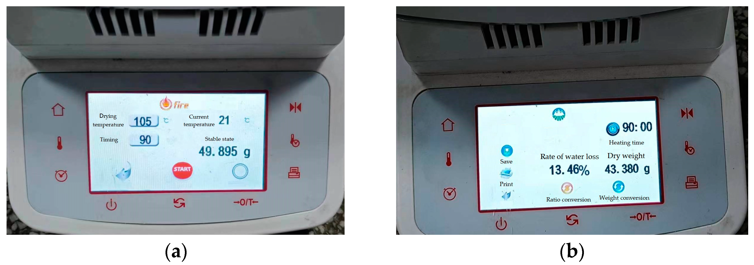
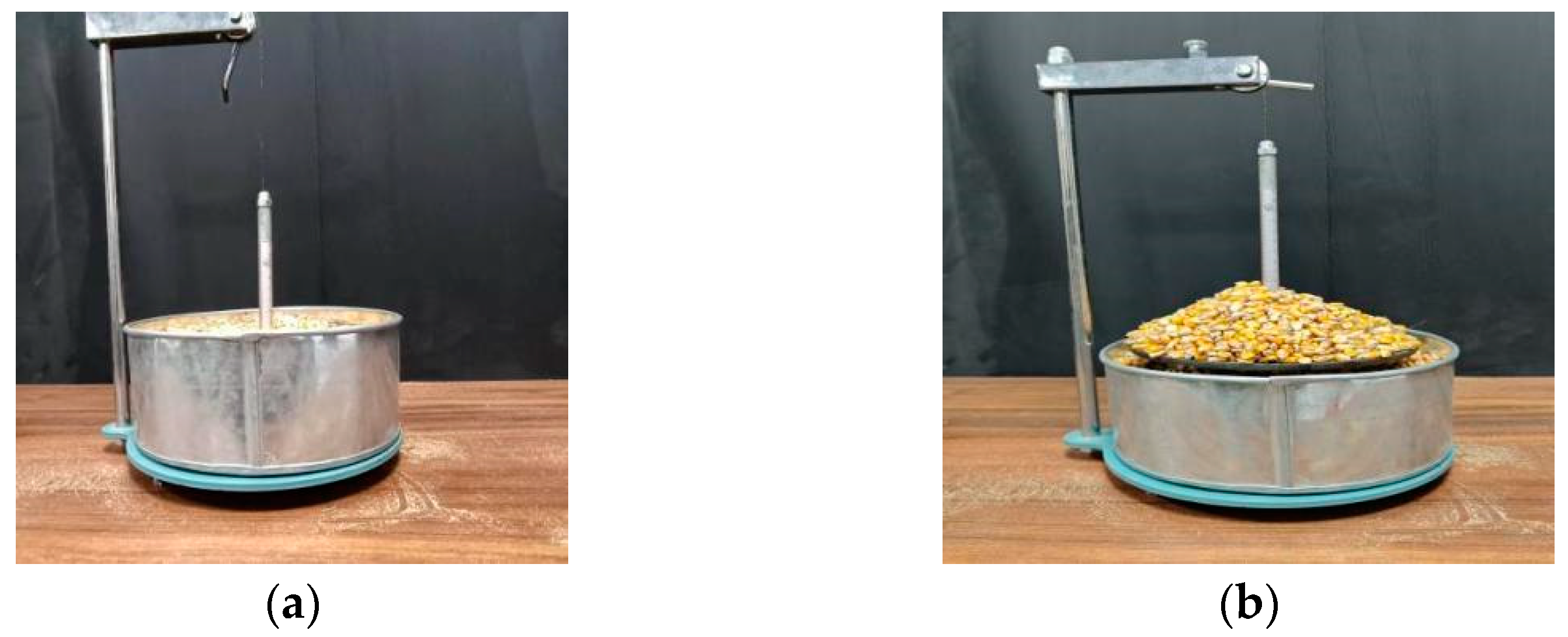
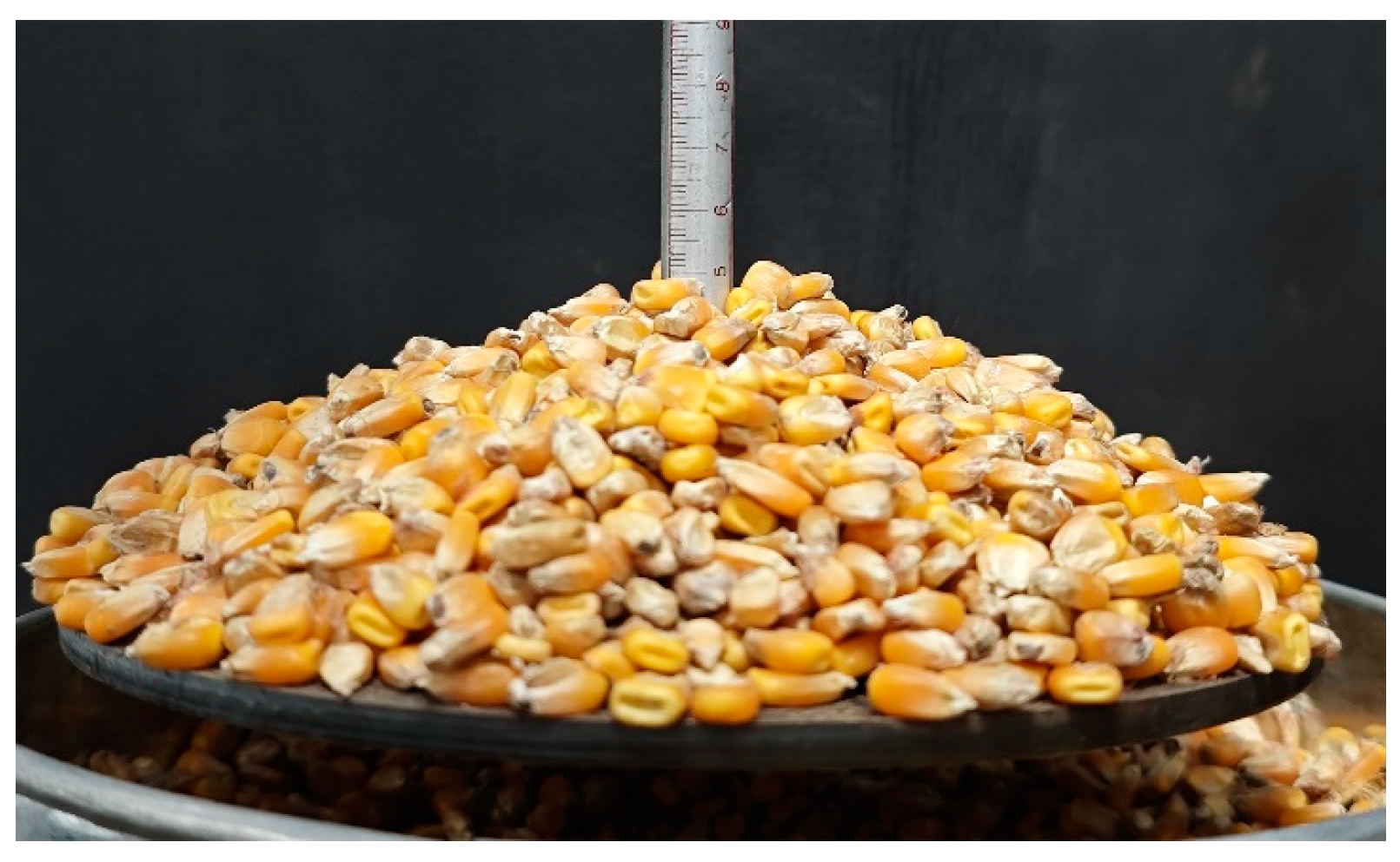
Funding

This research was funded by the National Key Research and Development Program of China, grant number 2022YFD2300803; Major Science and Technology Programs in Henan Province, grant number 221100110800; and Major Science and Technology Special Project of Henan Province (Longmen Laboratory First-class Project), grant number 231100220200.

Institutional Review Board Statement

Not applicable.

Data Availability Statement

The data presented in this study are available upon request from the corresponding author. The data are not publicly available.

Conflicts of Interest

The authors declare no conflicts of interest.

References

  1. Cundall, P.A.; Strack, O.D.L. A Discrete Numerical Model for Granular Assemblies. Géotechnique 1979, 29, 47–65. [Google Scholar] [CrossRef]
  2. Boac, J.M.; Ambrose, R.P.K.; Casada, M.E.; Maghirang, R.G.; Maier, D.E. Applications of Discrete Element Method in Modeling of Grain Postharvest Operations. Food Eng. Rev. 2014, 6, 128–149. [Google Scholar] [CrossRef]
  3. Anand, A.; Curtis, J.S.; Wassgren, C.R.; Hancock, B.C.; Ketterhagen, W.R. Predicting Discharge Dynamics of Wet Cohesive Particles from a Rectangular Hopper Using the Discrete Element Method (DEM). Chem. Eng. Sci. 2009, 64, 5268–5275. [Google Scholar] [CrossRef]
  4. Raji, A.O.; Favier, J.F. Model for the Deformation in Agricultural and Food Particulate Materials under Bulk Compressive Loading Using Discrete Element Method. II: Compression of Oilseeds. J. Food Eng. 2004, 64, 373–380. [Google Scholar] [CrossRef]
  5. Berger, R.; Kloss, C.; Kohlmeyer, A.; Pirker, S. Hybrid Parallelization of the LIGGGHTS Open-Source DEM Code. Powder Technol. 2015, 278, 234–247. [Google Scholar] [CrossRef]
  6. Wang, X.; Yu, J.; Lv, F.; Wang, Y.; Fu, H. A Multi-Sphere Based Modelling Method for Maize Grain Assemblies. Adv. Powder Technol. 2017, 28, 584–595. [Google Scholar] [CrossRef]
  7. Li, H.; Zeng, R.; Niu, Z.; Zhang, J. A Calibration Method for Contact Parameters of Maize Kernels Based on the Discrete Element Method. Agriculture 2022, 12, 664. [Google Scholar] [CrossRef]
  8. ANSYS. Rocky DEM Technical Manual; ANSYS: Canonsburg, PA, USA, 2022. [Google Scholar]
  9. Zhou, L.; Yu, J.; Liang, L.; Yu, Y.; Yan, D.; Sun, K.; Wang, Y. Study on Key Issues in the Modelling of Maize Seeds Based on the Multi-Sphere Method. Powder Technol. 2021, 394, 791–812. [Google Scholar] [CrossRef]
  10. Li, X.; Du, Y.; Liu, L.; Mao, E.; Wu, J.; Zhang, Y.; Guo, D. A Rapid Prototyping Method for Crop Models Using the Discrete Element Method. Comput. Electron. Agric. 2022, 203, 107451. [Google Scholar] [CrossRef]
  11. Chiaravalle, A.G.; Cotabarren, I.M.; Pina, J. DEM Breakage Calibration for Single Particle Fracture of Maize Kernels under a Particle Replacement Approach. Chem. Eng. Res. Des. 2023, 195, 151–165. [Google Scholar] [CrossRef]
  12. Han, D.-D.; Xu, Y.; Huang, Y.-X.; He, B.; Dai, J.-W.; Lv, X.-R.; Zhang, L.-H. DEM Parameters Calibration and Verification for Coated Maize Particles. Comp. Part. Mech. 2023. [Google Scholar] [CrossRef]
  13. Wang, L.; Zheng, Z.; Yu, Y.; Liu, T.; Zhang, Z. Determination of the Energetic Coefficient of Restitution of Maize Grain Based on Laboratory Experiments and DEM Simulations. Powder Technol. 2020, 362, 645–658. [Google Scholar] [CrossRef]
  14. Mousaviraad, M.; Tekeste, M.Z. Effect of Grain Moisture Content on Physical, Mechanical, and Bulk Dynamic Behaviour of Maize. Biosyst. Eng. 2020, 195, 186–197. [Google Scholar] [CrossRef]
  15. Xia, Y.; Klinger, J.; Bhattacharjee, T.; Aston, J.; Small, M.; Thompson, V. An Experiment-Informed Discrete Element Modelling Study of Knife Milling for Flexural Biomass Feedstocks. Biosyst. Eng. 2023, 236, 39–53. [Google Scholar] [CrossRef]
  16. Dong, J.; Zhang, D.; Yang, L.; Cui, T.; Zhang, K.; He, X.; Wang, Z.; Jing, M. Discrete Element Method Optimisation of Threshing Components to Reduce Maize Kernel Damage at High Moisture Content. Biosyst. Eng. 2023, 233, 221–240. [Google Scholar] [CrossRef]
  17. Li, X.; Du, Y.; Liu, L.; Mao, E.; Yang, F.; Wu, J.; Wang, L. Research on the Constitutive Model of Low-Damage Corn Threshing Based on DEM. Comput. Electron. Agric. 2022, 194, 106722. [Google Scholar] [CrossRef]
  18. Horabik, J.; Molenda, M. Parameters and Contact Models for DEM Simulations of Agricultural Granular Materials: A Review. Biosyst. Eng. 2016, 147, 206–225. [Google Scholar] [CrossRef]
  19. Coetzee, C.J. Review: Calibration of the Discrete Element Method. Powder Technol. 2017, 310, 104–142. [Google Scholar] [CrossRef]
  20. Coetzee, C.J.; Els, D.N.J. Calibration of Discrete Element Parameters and the Modelling of Silo Discharge and Bucket Filling. Comput. Electron. Agric. 2009, 65, 198–212. [Google Scholar] [CrossRef]
  21. Markauskas, D.; Ramírez-Gómez, Á.; Kačianauskas, R.; Zdancevičius, E. Maize Grain Shape Approaches for DEM Modelling. Comput. Electron. Agric. 2015, 118, 247–258. [Google Scholar] [CrossRef]
  22. Chen, Z.; Wassgren, C.; Ambrose, R.P.K. Development and Validation of a DEM Model for Predicting Impact Damage of Maize Kernels. Biosyst. Eng. 2022, 224, 16–33. [Google Scholar] [CrossRef]
  23. Su, Y.; Xu, Y.; Cui, T.; Gao, X.; Xia, G.; Li, Y.; Qiao, M. Determination and Interpretation of Bonded-Particle Model Parameters for Simulation of Maize Kernels. Biosyst. Eng. 2021, 210, 193–205. [Google Scholar] [CrossRef]
Figure 1. Determination of moisture content in maize kernels. The setting (a) and the result (b).
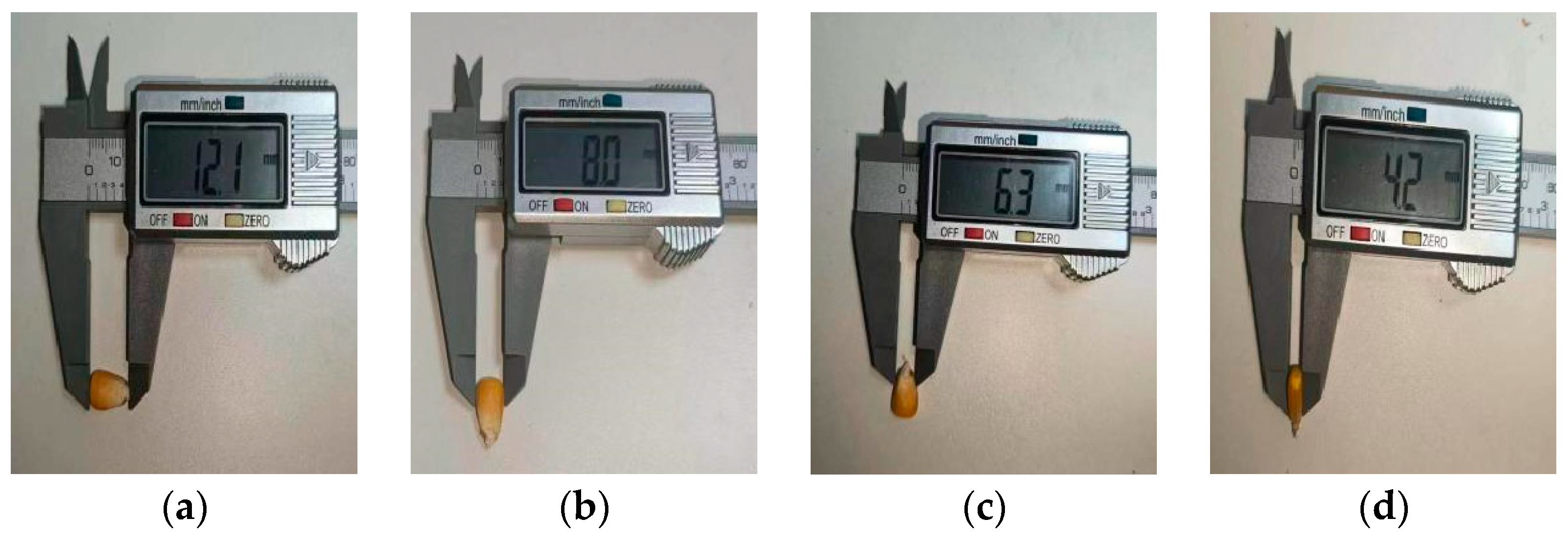
Agriculture 14 00587 g001
Figure 2. The measurement process of maize total length (a), upper width (b), lower width (c), and thickness (d).
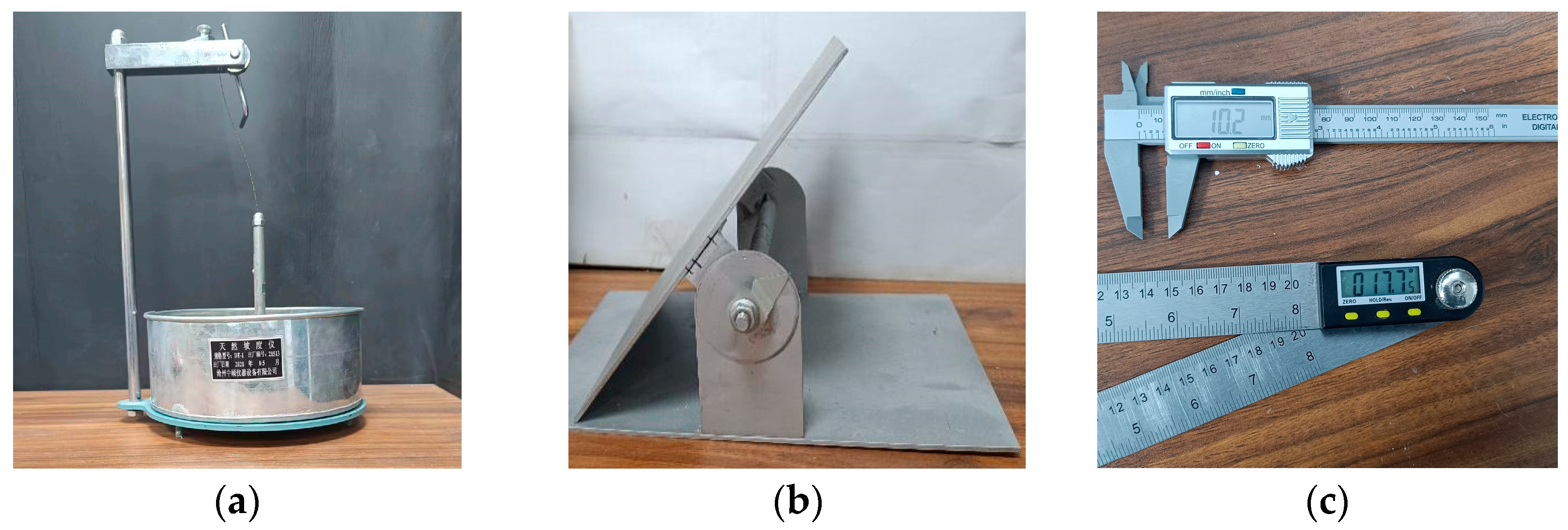
Agriculture 14 00587 g002
Figure 3. The test equipment consist of a DT-1 natural slope meter (a), electronic vernier caliper and inclined plate (b), and digital protractor (c) for the slope sliding method and slope rolling method.
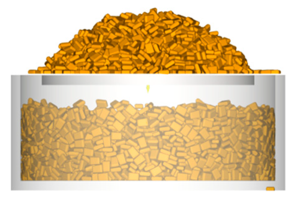
Agriculture 14 00587 g003
Figure 5. The test process of the real stacking angle. The initial state (a) and final state (b).
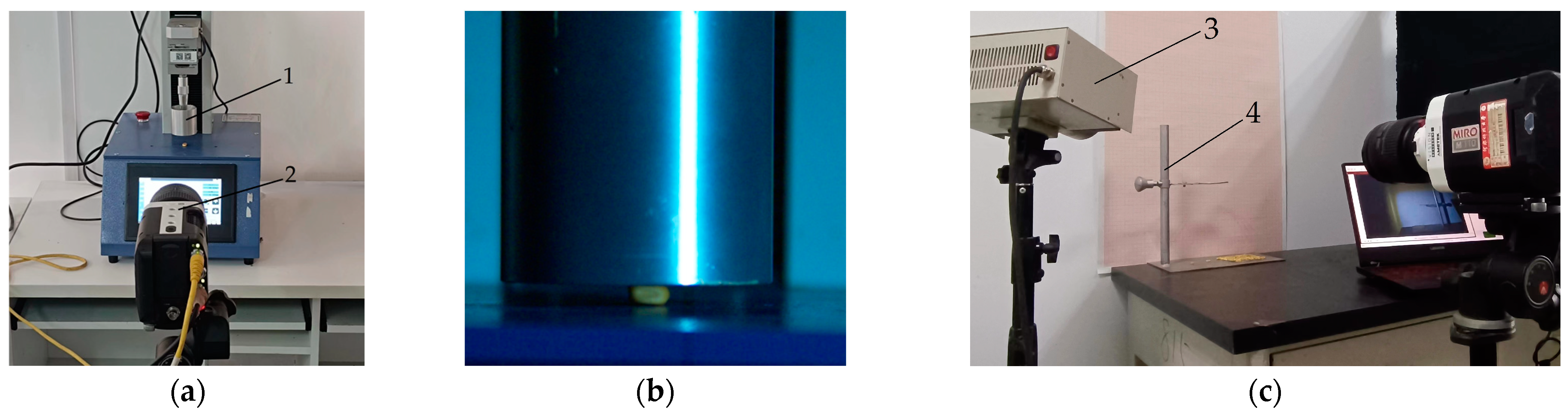
Agriculture 14 00587 g005
Figure 6. The measurement process of some parameters. The Poisson’s ratio of the kernel (a), the Young’s modulus of the kernel (b) and the recovery coefficients (c). 1. Texture analyzer; 2. High-speed camera; 3. Fill light; 4. The stand.
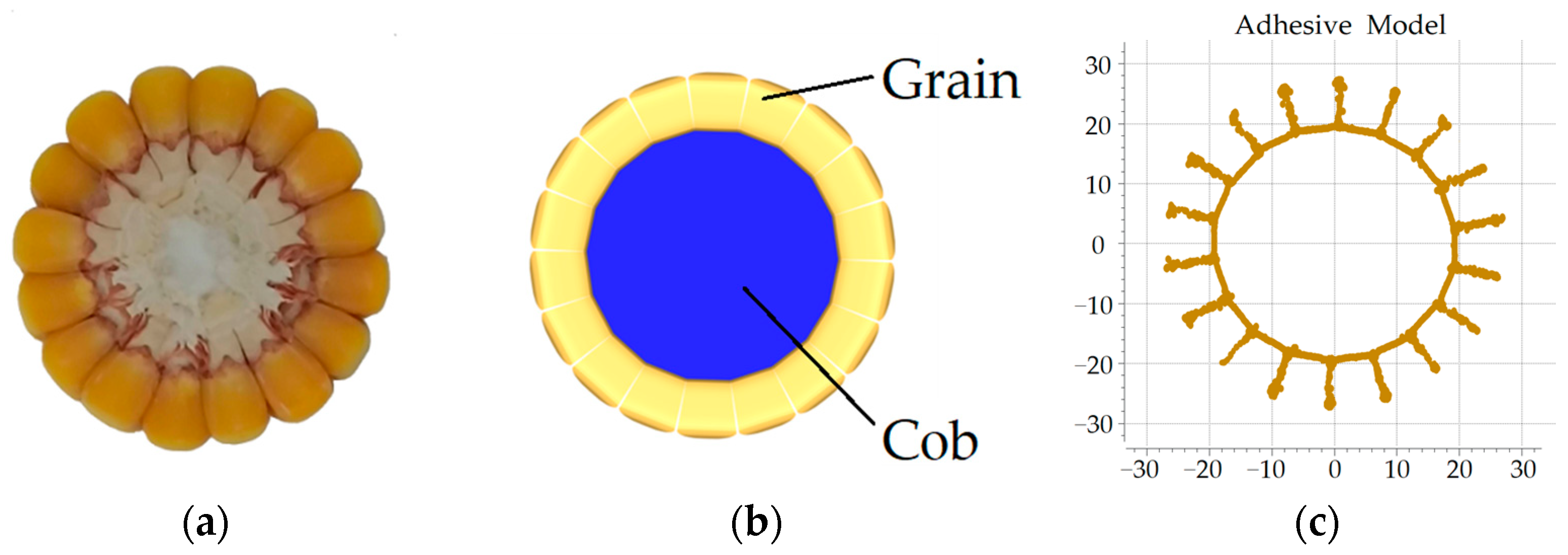
Agriculture 14 00587 g006
Figure 7. The actual maize image (a), the combination model of grain and cob (b), and the adhesive force model (c).
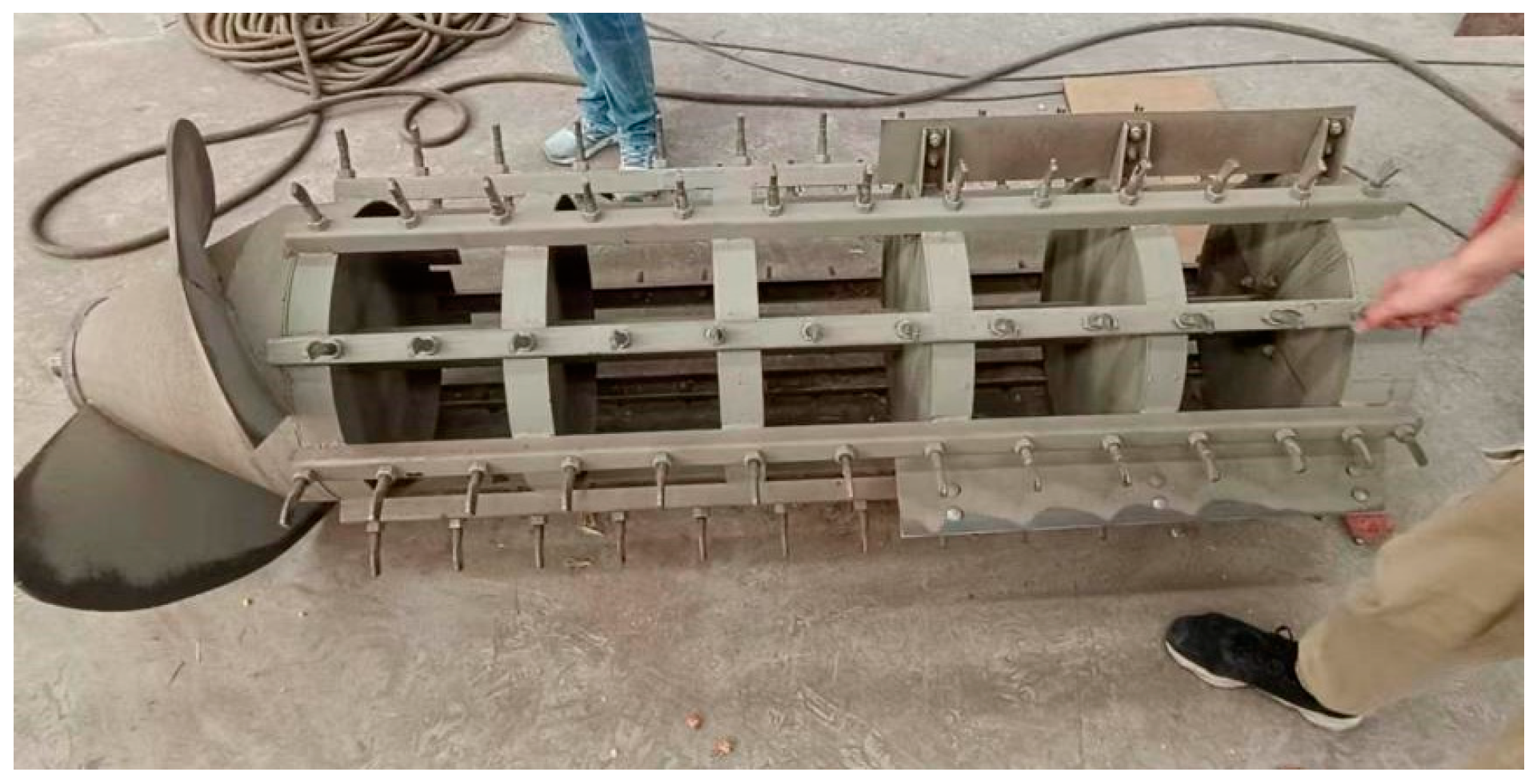
Agriculture 14 00587 g007
Figure 8. The actual threshing cylinder.
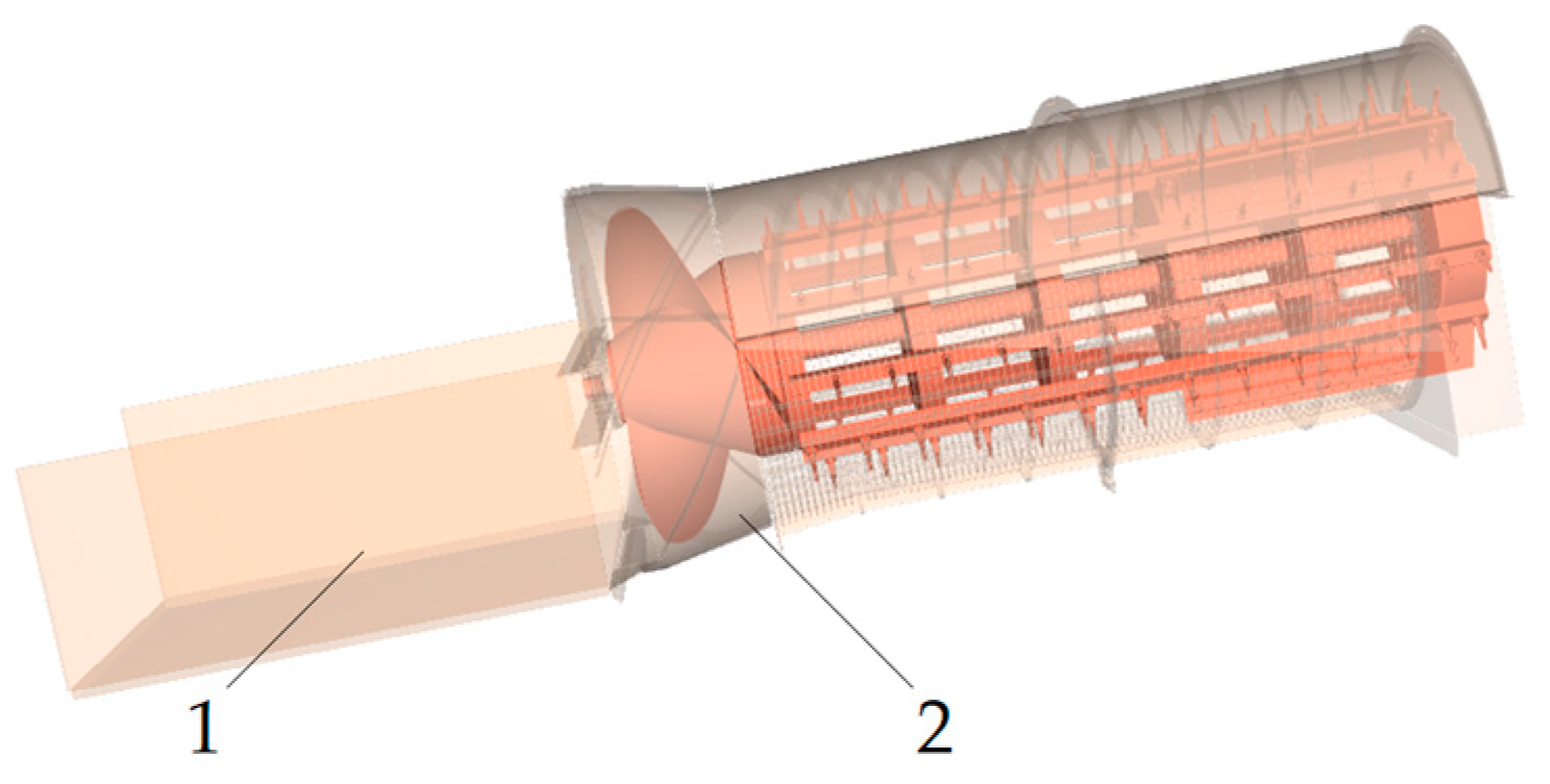
Agriculture 14 00587 g008
Figure 9. The single longitudinal axial flow threshing device model. 1. Conveyor belt; 2. Threshing device.
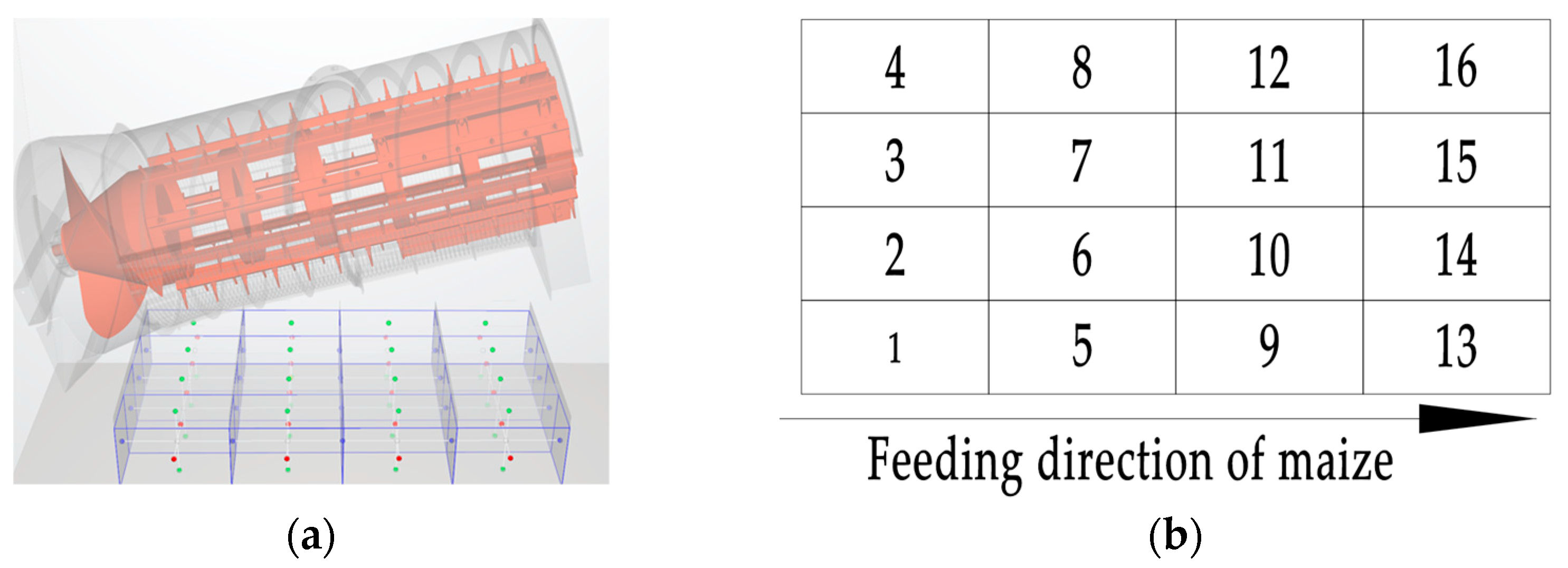
Agriculture 14 00587 g009
Figure 10. The 4 × 4 equal-area segmentation granary: (a) overall schematic diagram; (b) the vertical view.
Agriculture 14 00587 g010
Figure 11. The result of the actual stacking angle test.
Agriculture 14 00587 g011
Figure 12. The result of the first test.
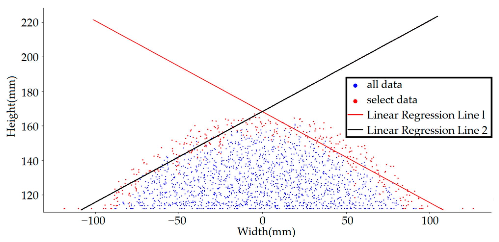
Agriculture 14 00587 g012
Figure 13. The linear analysis of the first test.
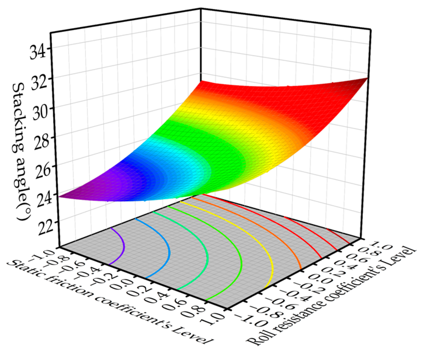
Agriculture 14 00587 g013
Figure 14. The response surface of the influence of A and B on the stacking angle.
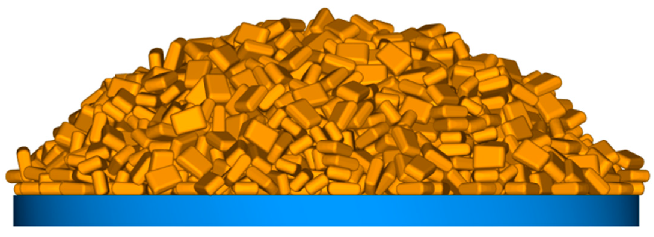
Agriculture 14 00587 g014
Figure 15. The test of the optimal calibration parameter.
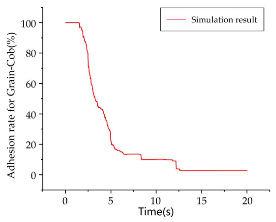
Agriculture 14 00587 g015
Figure 16. The adhesion rate of maize kernels–cob model.
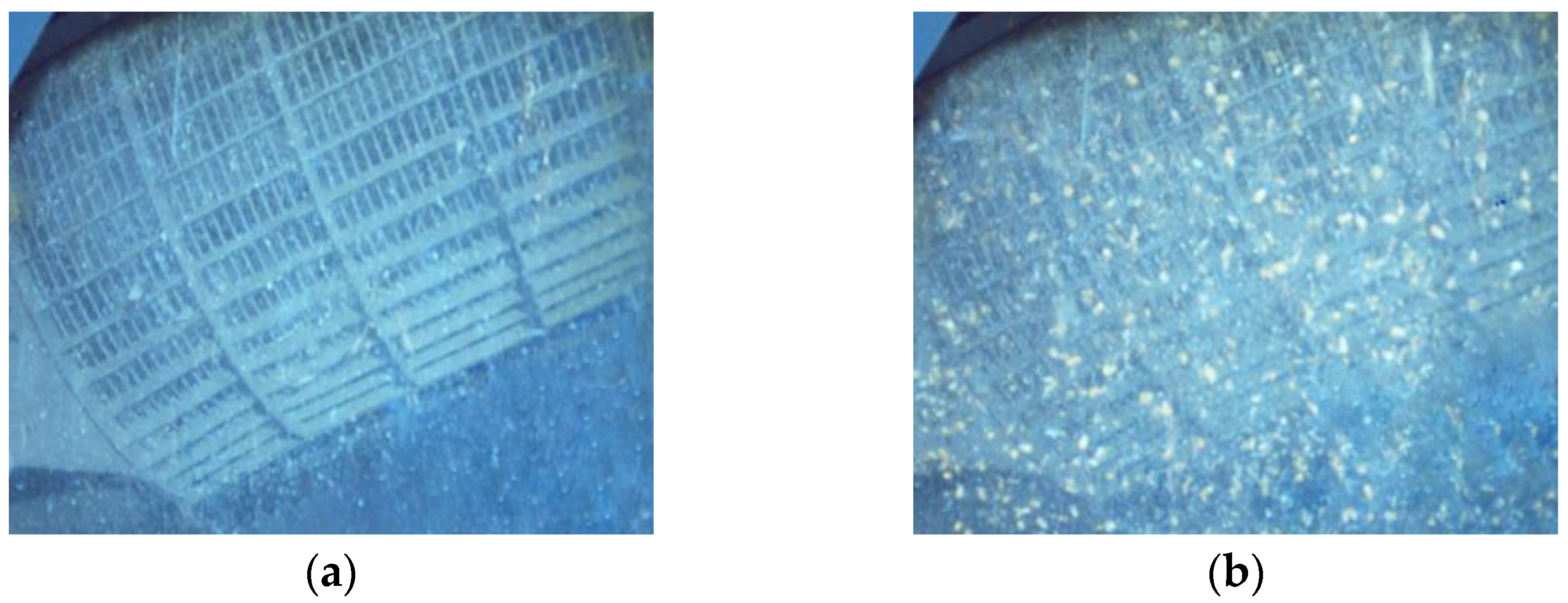
Agriculture 14 00587 g016
Figure 17. The actual test process of maize threshing. (a). Threshing at 2 s (b). Threshing at 8 s.
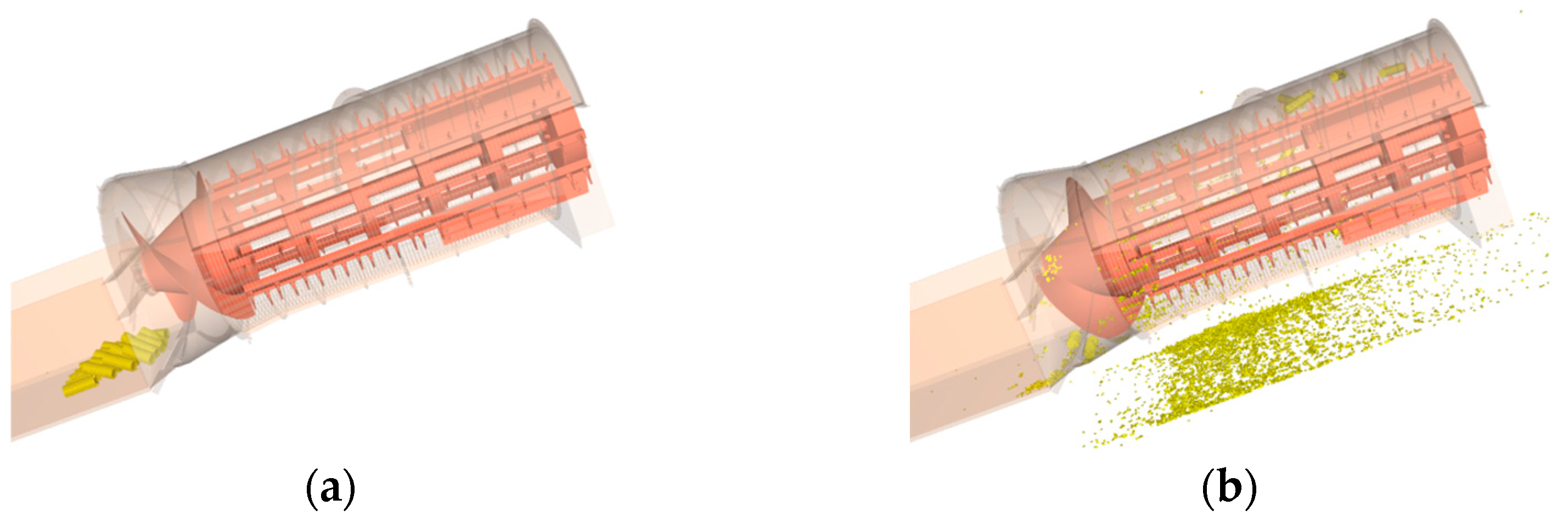
Agriculture 14 00587 g017
Figure 18. The simulation test process of maize threshing. (a). Threshing at 2 s (b). Threshing at 8 s.
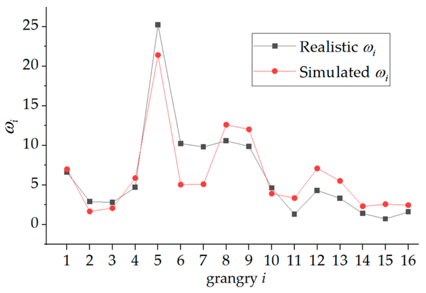
Agriculture 14 00587 g018
Figure 19. The point line image of the actual–simulation test.
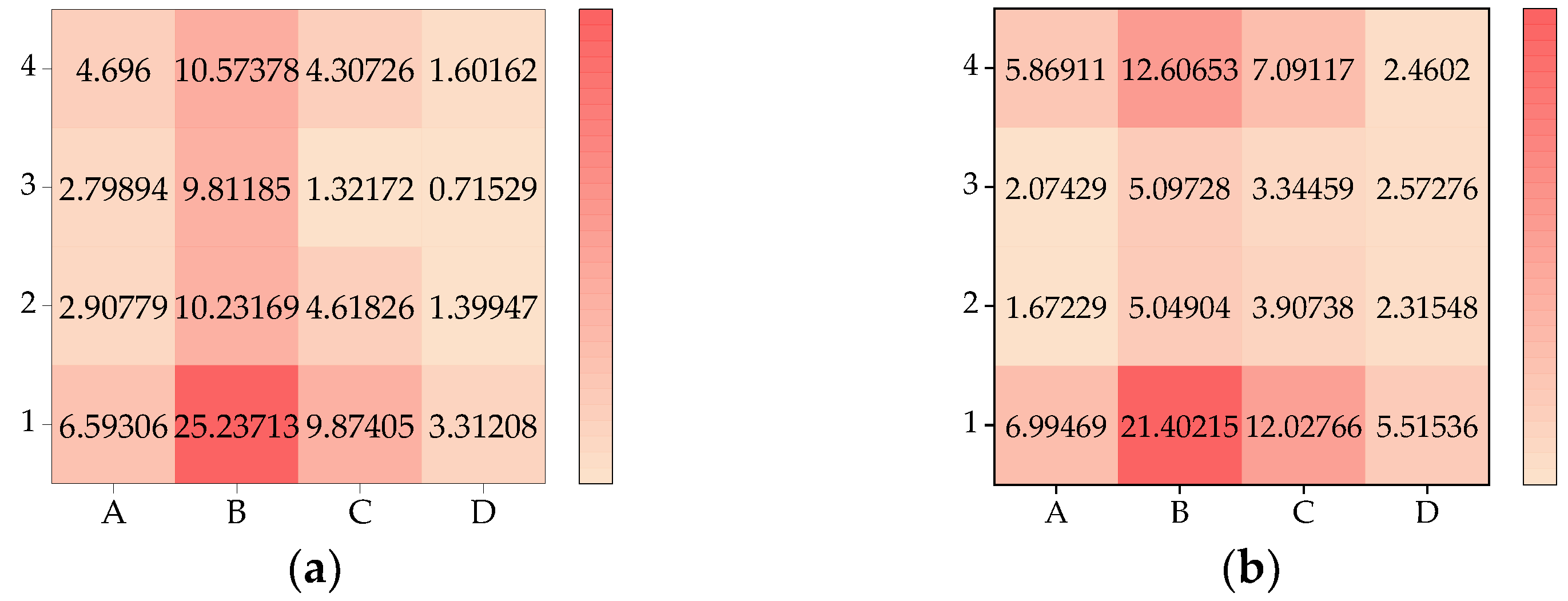
Agriculture 14 00587 g019
Figure 20. The heat maps of the actual results (a) and the simulation results (b).
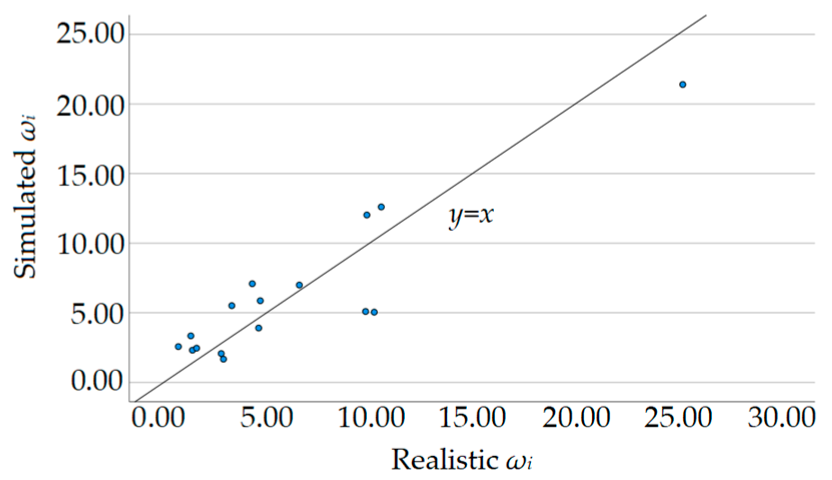
Agriculture 14 00587 g020
Figure 21. The scatterplot of the relationship between the actual results and simulation results.
Agriculture 14 00587 g021
Table 1. The classification of maize grain shape.
Grain ShapeGrain NumbersProportion
horse-tooth16281%
truncated triangular pyramid2311.50%
ellipsoidal cone42%
spheroid31.50%
irregular31.50%
broken52.5%
Table 2. The results of maize measurement.
SizeAverage (mm)
Total length11.1
Upper width8.1
Lower width7
Thickness4.5
Table 3. The determination of the static friction coefficient.
ResultsStatic Friction Coefficient
Maximum0.67
Minimum0.46
Average0.56
Standard deviation0.06
Table 4. The determination of the roll friction coefficient.
ResultsRoll Resistance Coefficient
Maximum0.133
Minimum0.070
Average0.104
Standard deviation0.021
Table 5. The settings of relevant parameters.
ParametersValue
Poisson’s ratio of kernel0.4
Young’s modulus of kernel116.91 MPa
Kernel density1197 Kg/m3
Kernel–Kernel recovery coefficient0.233
Kernel–Steel recovery coefficient0.6
Static friction coefficient of kernel–steel0.46
Poisson’s ratio of steel plate0.29
Young’s modulus of steel plate206 GPa
Steel plate density8000 Kg/m3
Table 6. The level of the two factors in the simulation test.
LevelStatic Friction CoefficientRoll Resistance Coefficient
−10.410.054
00.560.104
10.710.154
Table 7. The simulation parameters of the machine working in the threshing process.
ParametersValue
Rotational speed of threshing cylinder400 Rpm
Conveying speed of conveyor belt0.8 m/s
Maize feeding amount10 Kg/s
Simulation duration20 s
Table 8. The results of the actual stacking angle test.
ResultsGauge Reading (mm)Stacking Angle (DEG)
Average52.427.646
Standard deviation2.321.040
Table 9. The final stacking angle results of the simulation test.
StdStatic Friction
A
Dynamic Friction
B
Stacking Angle (DEG)
11−127.75
20−125.5
30024.8
41028.1
5−1−123.3
6−1026.7
70023.9
8−1129.1
91131.8
100130.1
110028.2
120027.9
130026.9
Table 10. The results of the model analysis of variance.
SourceSum of SquaresdfMean SquareF-Valuep-ValueSignificance
Model57.2511.445.030.0284*
A14.57114.576.40.0392*
B35.28135.2815.50.0056**
AB0.525610.52560.23090.6455-
0.751310.75130.330.5836-
3.7913.791.670.2379-
Residual15.9472.28 -
Lack of fit1.430.46780.12880.9381-
Pure error14.5343.63
Cor total73.1312
* means significant influence in the 95% confidence interval. ** means significant influence in the 99% confidence interval. – means no significant influence.
Table 11. The ratio of the mass in each granary to the total mass.
Granary i Realistic   ω i Simulated   ω i
16.596.99
22.911.67
32.802.07
44.705.87
525.2421.40
610.235.05
79.815.10
810.5712.61
99.8712.03
104.623.91
111.323.34
124.317.09
133.315.52
141.402.32
150.722.57
161.602.46
Table 12. The calculation process of the Wilcoxon signed-rank test.
Granary i Realistic   ω i Simulated   ω id R i + R i
16.596.990.41-
22.911.67−1.24-−7
32.82.07−0.73-−3
44.75.871.176-
525.2421.4−3.84-−14
610.235.05−5.18-−16
79.815.1−4.71-−15
810.5712.612.0410-
99.8712.032.1611-
104.623.91−0.71-−2
111.323.342.029-
124.317.092.7813-
133.315.522.2112-
141.42.320.925-
150.722.571.858-
161.62.460.864-
Total T + = 79 T = 57
Disclaimer/Publisher’s Note: The statements, opinions and data contained in all publications are solely those of the individual author(s) and contributor(s) and not of MDPI and/or the editor(s). MDPI and/or the editor(s) disclaim responsibility for any injury to people or property resulting from any ideas, methods, instructions or products referred to in the content.

