Design and Test of Hydraulic Driving System for Undercarriage of Paddy Field Weeder

Abstract

In response to challenges such as inadequate driving stability and power in traditional weeding machinery, we designed and investigated a hydraulic chassis tailored for paddy field operations. Utilizing SolidWorks and RecurDyn V9R4 software, we obtained linear driving and steering curves to model and simulate the dynamics of the mower chassis. Through the AMESim software, we further modeled and simulated the hydraulic chassis system, focusing on the hydraulic characteristics of the components relevant to its operation. Subsequently, we developed a hydraulic-driven paddy weeder and conducted tests to evaluate the linear deviation and paddy slip rates. Our findings indicate that the designed hydraulic weeder chassis exhibits commendable dynamic performance and driving stability, with the actual average deviation and paddy slip rates measured at 2.61% and 3.59%, respectively. These results underscore the efficacy of our approach in addressing the challenges inherent in traditional weeding machinery and highlight the potential of hydraulic systems in enhancing agricultural operations.

1. Introduction

Rice cultivation holds a paramount position in global food production [1], predominantly in Asia, where nearly 90% of the world’s rice sowing area and output are concentrated [2]. However, weed infestation poses a significant threat, causing annual yield reductions of over 15% [3,4]. Conventional methods such as chemical herbicides exhibit low efficacy and substantial environmental harm [5,6]. Consequently, the development of innovative agricultural machinery is imperative to enhance land productivity sustainably.

In Europe, the US, and other countries, rice planting mostly uses air seeding, seedling growth is chaotic, and agricultural tools such as weeding machines are inapplicable [7]. Therefore, chemical weeding is the main solution to field grass damage. Most rice planting methods in Asian countries include mechanical transplanting, seedling growth is organized, and mechanical weeding can be used to control weeds [8]. Existing paddy field weeding machines are mainly divided into two types according to the walking mode: the step type and ride type. Step weeding machines are mainly Japanese and the same as industry MSJ-type and Meishan SMW models [9], Wang et al.’s [10] organic rice weeding machine, and Qi et al.’s [11] research and development of a step-type paddy field weeding machine. The riding weeder is typically operated approximately seven rows each time, and the work efficiency is relatively high. These weeders are mainly Japanese Yanma SJVP series, Mitsubishi Agricultural Machinery LW-8, real industry RW50 and other models [12], and the 2BYS-6 paddy field weeding machine [13] developed by Nanjing Agricultural Mechanization Research Institute, most of which use a traditional chassis as the carrying unit [14,15]. However, the traditional chassis has the following disadvantages: (1) the transmission system is complex and bulky, increasing the complexity of its adaption to the working condition of the paddy field with poor bearing capacity, and the layout is fixed and single; (2) failure to realize continuous speed change; and (3) achieving automation and intelligent control is also difficult [16,17].

Compared with traditional mechanical transmission, hydraulic drive technology has an excellent power-to-mass ratio, fast response, flexible layout, and direct implementation of intelligent control [18]. The hydraulic transmission system can provide higher power at a relatively light weight, which enables the weeder to achieve greater work efficiency while maintaining the light weight. The hydraulic-driven weeding machine can quickly adjust the height of the weeding disc according to soil conditions, thereby achieving precise weeding.

This paper addresses the limitations of existing paddy field weeders by proposing a novel hydraulic-driven chassis. Through 3D modeling, dynamic simulation, and comprehensive testing, the hydraulic chassis driving system is meticulously examined. Key advancements include enhanced steering flexibility and a reduced turning radius achieved through hydraulic steering, contributing to improved maneuverability in challenging paddy field conditions [19,20]. Additionally, this study conducts ground driving offset distance and paddy field slip rate tests, providing insights into the performance of the hydraulic chassis under various operating scenarios.

2. System Structure and Working Principle

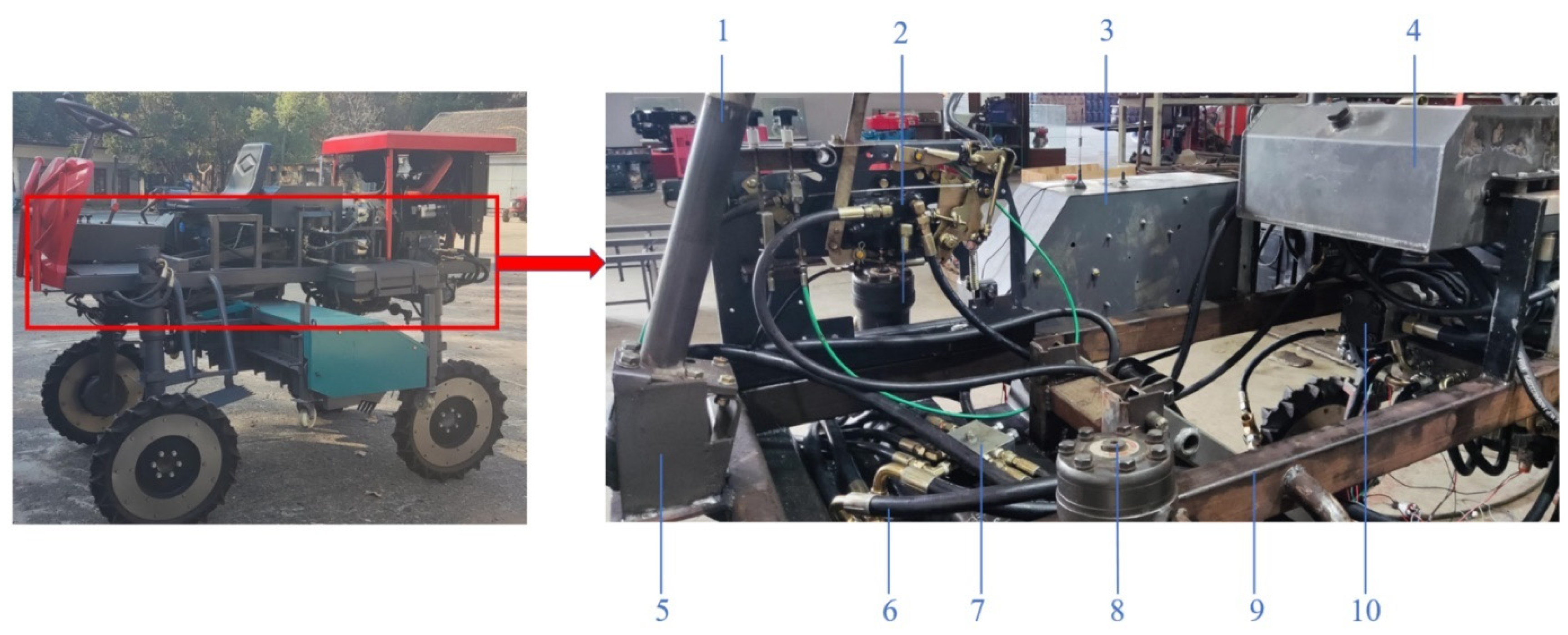
2.1. Chassis Structure

The chassis of a paddy field weeder is mainly composed of a chassis steel frame, fixed device, and driving wheel. A diesel engine, hydraulic oil pump (double pump), hydraulic tank, diverter valve, hydraulic motor, reversing valve, cooling device, and filter are all included in the hydraulic drive system. The field weeder is composed of two hydraulic fuel tanks and two separate hydraulic systems. One set is responsible for the walking and hydraulic lifting device of the weeder, and the other set is used for the steering system of the weeder. Under the premise of ensuring the balanced operation of the weeder, the weeder device is installed in the middle of the weeder due to the particularity of paddy fields, and the hydraulic lifting device is connected with the chassis of the weeder. Only the driving system is designed in this paper, and only the hydraulic interface can be provided for the hydraulic lifting system (Figure 1).

2.2. Working Principle

A four-wheel drive is adopted by the designed paddy field weeder. The capability to adapt to highly complex land and road conditions and the strong obstacle crossing and anti-slip performance, which is suitable for paddy field work, are the main advantages of four-wheel drive [21,22]. The weed wheel is driven by four hydraulic motors, and the mechanical energy of the diesel engine is converted to the pressure energy of the hydraulic oil using double pumps. The inside and outside flow of the hydraulic motor and the direction of operation are controlled by the diverter and reversing valves, respectively, to complete the weeder forward, backward, and steering functions. The relevant technical parameters of the weeder are shown in

Table 1. Main technical parameters of paddy field weeder chassis.

Argument	Value/Type
Machine size (length × width × height)/(mm × mm × mm)	2080 × 1650 × 1020
Overall quality/kg	1000
Supporting power/kw	15
Driving mode	Four-wheel drive
Steering mode	Differential steering
Minimum adaptive line spacing/mm	300
Working width/mm	1985
Adaptive plant spacing/mm	100

.

3. Walking Hydraulic System Design

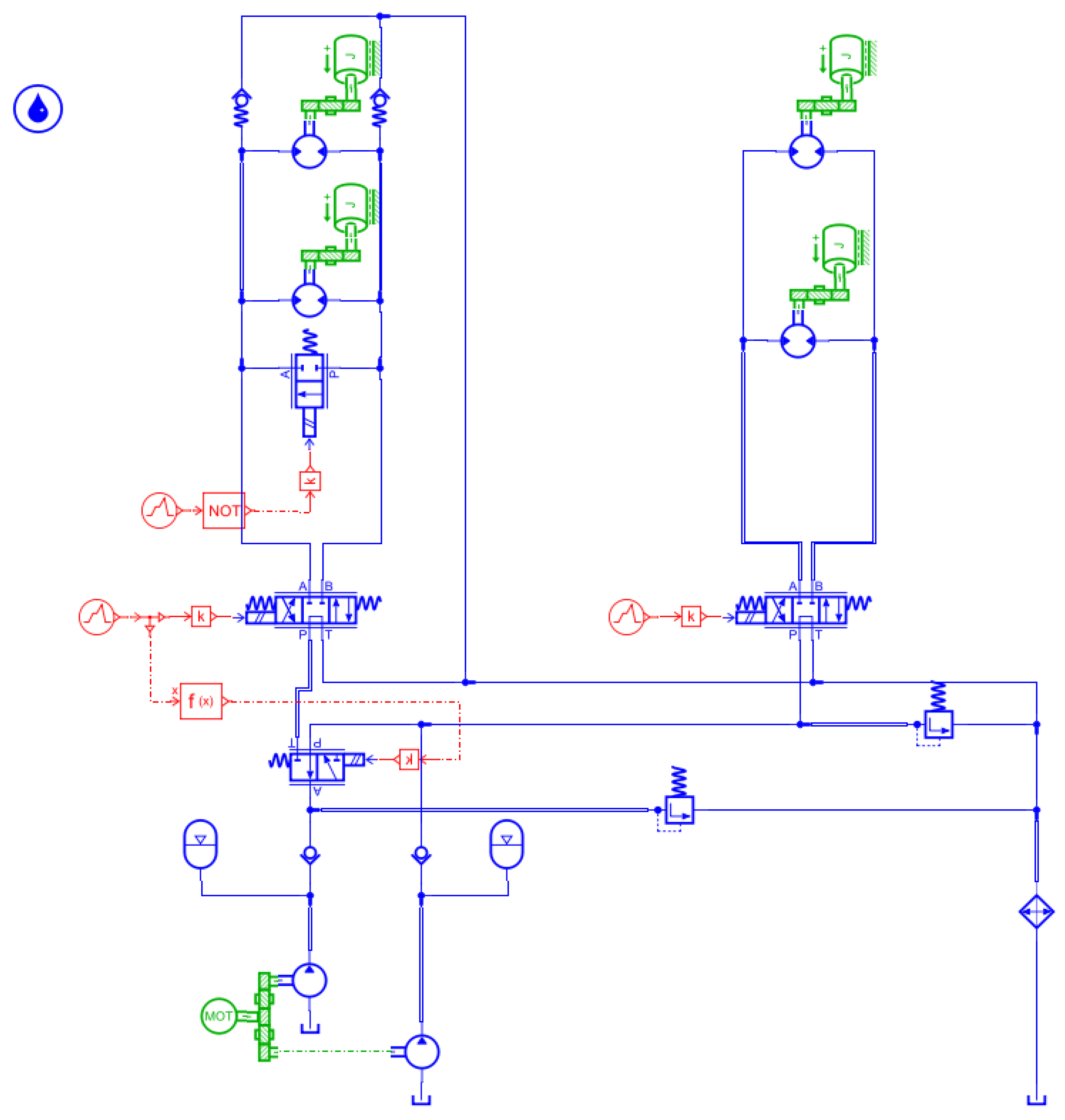
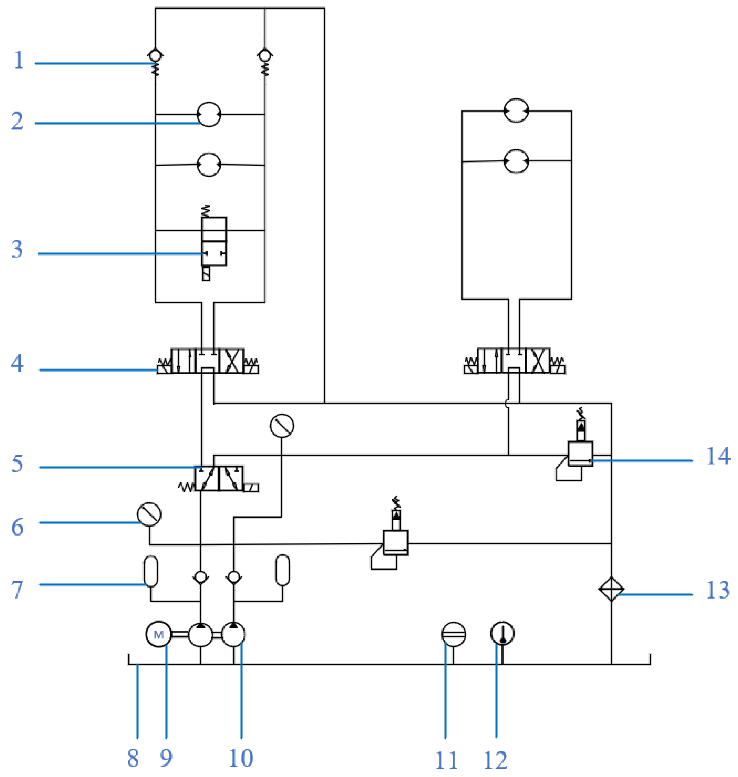
3.1. Principle of Hydraulic System

The principal diagram of the fully hydraulic chassis drive system designed in this paper is shown in Figure 2.

The power transmission process begins with the engine (9), which supplies mechanical power to the double pump (10). This double pump is pivotal, as it serves as the heart of the hydraulic system, pumping hydraulic oil to the system’s components. Its dual-pump design is strategic, allowing for the separation of the hydraulic circuits that operate the weeder’s various functions. This division enhances the system’s efficiency and reliability, as each circuit can be optimized for its specific task without imposing load or operational constraints on the other.

A critical component in managing the flow and direction of the hydraulic oil is the two-position three-way directional valve (5). By altering the flow direction, this valve facilitates the seamless switching between oil circuits, enabling the hydraulic system to adapt swiftly to changing operational needs. This adaptability is crucial for precision tasks in the paddy field.

For the control of the chassis’s movement, including forward and reverse motions, the three-position four-way solenoid directional valve (4) is utilized. This valve’s ability to adjust the hydraulic motor’s direction ensures that the chassis can navigate effectively through the paddy fields, offering both flexibility and control in maneuvering.

The integration of the two-position two-way solenoid directional valve (3) allows for precise on–off control of the hydraulic flow, effectively managing the chassis’s movement commands. This precise control is essential for stopping the chassis, highlighting the system’s responsiveness to operator inputs.

Safety and system integrity are ensured by the check valve (1), which prevents the backflow of hydraulic oil, safeguarding the system against potential damage. The monitoring and maintenance of the hydraulic system are facilitated by several key components: the pressure gauge (6) monitors the circuit pressure, the accumulator (7) stabilizes the energy and balances the pressure fluctuations, and the level gauge (11) measures the hydraulic oil height in the cylinder (8), ensuring optimal operation. Thermal management is addressed by the thermometer (12), which provides temperature readings, and the temperature regulator (13), which cools overheated oil, maintaining the system’s efficiency and preventing damage. The relief valve (14) plays a vital role in maintaining system pressure, ensuring the hydraulic system operates within its safe operating parameters.

The decision to deploy two separate hydraulic systems within the weeder stems from the need for operational redundancy and specialization. This dual-system approach allows for the separation of the weeder’s locomotion and operational functions, enhancing performance efficiency and minimizing the risk of system failure impacting the entire device.

The integration of the fixed device and driving wheel into the chassis structure, and their role in the overall functioning, are designed with the paddy field’s unique challenges in mind. The fixed device ensures stability during operation, essential in the uneven and muddy terrain of paddy fields. The driving wheel’s design and placement are optimized for maximum traction and minimal soil compaction, ensuring the weeder moves smoothly without damaging the crop.

3.2. Calculation and Selection of Main Power Components

3.2.1. Calculation of Maximum Driving Resistance

The driving conditions of the weeder should be met:

$$F\ge F_{ f}+F_{ w}+F_{ g}+F_{ a}$$

(1)

where $F$ is the traction force (N), $F_{ f}$ is the rolling resistance (N), $F_{ w}$ is the air resistance (N), $F_{ g}$ is the slope resistance (N), and $F_{ a}$ is the acceleration resistance (N).

When the weeder works in a paddy field, the rolling resistance $F_{ f}$ is the product of the normal supporting force of the ground and the rolling resistance coefficient. The slope resistance $F_{ g}$ is the product of the total mass of the weeder and the slope, and the air resistance $F_{ w}$ is related to the frontal windward area, body shape, and fuselage material of agricultural machinery and increases in a square relationship with the speed. The air resistance is remarkably small and ignorable for medium–low speed off-highway driving machinery with a maximum speed of no more than 50 km/h [23]. The maximum speed of the weeder does not exceed 10 km/h; therefore, its air resistance is disregarded in the calculation.

Rice fields typically have flat terrain, resulting in negligible slope resistance during the operational process. The calculation formula of the slope resistance is as follows:

$$F_{ g}=G\mathit{cos}\alpha$$

(2)

The acceleration resistance $F_{ a}$ refers to the comprehensive inertial resistance of the vehicle caused by speed changes, including the inertial resistance parallel to the driving direction accelerated by the vehicle body as a translational mass and the inertial resistance converted to improve the torque increment of the rotating mass speed of the wheel and other interior vehicles. The acceleration resistance is generally small in the medium–low speed vehicles and machinery driven by the hydrostatic pressure. In the actual calculation process, the acceleration resistance $F_{ a}$ is:

$$F_{ a}=\lambda mg$$

(3)

where $m$ is the overall quality (Kg), $g$ is the acceleration of gravity (m/s²), and $\lambda$ is the acceleration coefficient, which is numerically equal to the ratio of the actual acceleration to the gravitational acceleration.

Some parameters of the hydraulic chassis of the weeder can be designed by calculating the driving resistance of the weeder. The rolling resistance coefficient $f$ and the maximum adhesion coefficient $\mu$ of different road surfaces are presented in

Table 2. Rolling resistance coefficient $f$ and maximum adhesion coefficient $\mu$ of different road conditions.

Pavement	Peculiarity	Rolling Resistance Coefficient f	Maximum Adhesion Coefficient μ
Land for cultivation	Relatively soft	0.10–0.250	0.40–0.50
Wet mud floor	Changes in resistance, deep wheel printing	0.10–0.15	0.50–0.60
Paddy field	Drive wheel touches the bottom of the plow	0.20–0.25	0.35–0.50
Concrete pavement	Hardly any wheel marks	0.01–0.02	0.80–0.90

.

During paddy field operation, the mass of the weeder is generally 1000 kg, and the upper limit of the rolling resistance coefficient $f$ in the paddy field is 0.25. A paddy field is generally flat; thus, its driving slope can be ignored. The acceleration coefficient of 0.035 is taken and then substituted into Equation (2) to calculate the acceleration resistance $F_{ a}$ = 171.5 N and rolling resistance $F_{ g}$ = 0 N. Simultaneously, the full load gravity of the weeder and the maximum rolling resistance coefficient of the paddy field are inputted into Equation (1). The maximum traction force $F_{ max}$ of the paddy field of the weeder during operation is 2793 N, that is, the maximum driving resistance $F$ = 2793 N. When the weeder walks on the ground, the rolling resistance coefficient is small due to the superiority of the road condition to the paddy field, and the total resistance of the entire machine is less than the total resistance of the paddy field. Therefore, 2793 N is the maximum total driving resistance of the weeder under various working conditions.

3.2.2. Hydraulic Drive Motor Selection Calculation

The required torque for the traveling drive motor is:

$$M=\frac{FR}{m\alpha { }_1}$$

(4)

where $M$ is the required torque for a single hydraulic motor (N·m), $R$ is the driving wheel radius with a value of 0.3 m, $m$ is the number of drive motors with a value of 4, and ${\alpha }_{ 1}$ is the wheel drive efficiency, ${\alpha }_{ 1}$ = 0.91.

The theoretical displacement of the traveling drive motor is:

$$V_{ m}=\frac{2\pi M}{P\alpha { }_2}$$

(5)

where $V_{ m}$ is the theoretical displacement of the travel drive motor (mL/r), $P$ is the maximum allowable pressure of the hydraulic system with a value of 20 MPa, and ${\alpha }_{ 2}$ is the mechanical efficiency of walking hydraulic motor, ${\alpha }_{ 2}$ = 0.93.

The selected hydraulic motor should not only meet the maximum torque of the driving wheel but also the maximum driving speed of 3.6 km/h under the conditions of the small torque and high speed of the weeder. Therefore, the maximum speed of the hydraulic motor is calculated as follows:

$$n_{ max}=\frac{{1000v}_{ max}}{60\times 2\pi R}$$

(6)

where $n_{ max}$ is the maximum speed of the hydraulic motor (r/min), and $v_{ max}$ is the maximum speed of the weeder (km/h).

Combining Formula (1) with Formula (6), the maximum driving resistance of the weeder is 2793 N, the maximum torque of a single driving wheel is 230.2 N·m, the theoretical displacement of the hydraulic motor is calculated as 77.8 mL/r, and the maximum speed required by the hydraulic motor is 31.8 r/min. Therefore, the required flow rate of the hydraulic motor is roughly 2.5 L/min. Ultimately, the BMR-80 series cycloidal hydraulic motor was selected, and the motor parameters are presented in

Table 3. Hydraulic motor parameters.

Quality Characteristic	Argument
Equivalent displacement (mL/r)	81.5
Maximum working pressure (MPa)	22.5
Maximum speed (rpm)	650
Maximum discharge (L/min)	55
Maximum output torque (N·m)	650

.

3.2.3. Hydraulic Pump Selection Calculation

The model of the double pump is determined in accordance with the total flow of the oil circuit in the hydraulic system and the engine speed. According to the theoretical maximum displacement of the motor above 77.8 mL/r, the maximum operating speed of 2.5 km/h, and the engine speed of 3000 r/min, the output flow of the dual pump is calculated as follows:

$$Q_{ b}=\frac{{4V}_{ mmax}{n}_{ max}}{{1000\alpha }_{ 3}}$$

(7)

$$V_{ b}=\frac{{1000Q}_{ b}}{n_{ b}{\alpha }_{ 4}}$$

(8)

where $Q_{ b}$ is the hydraulic pump output flow (L/min), $V_{ mmax}$ is the maximum displacement of the hydraulic motor (mL/r), ${\alpha }_{ 3}$ is the volumetric efficiency of the hydraulic motor with a value of 0.95, $V_{ b}$ is the theoretical displacement of the hydraulic pump (mL/r), $n_{ b}$ is the hydraulic pump speed (r/min), and ${\alpha }_{ 4}$ is the volumetric efficiency of the hydraulic pump with a value of 0.95.

The total output flow of the hydraulic system is 10.4 L/min, and the theoretical displacement of the hydraulic pump is 10.9 mL/r.

According to the above calculation, combined with the selection principle of a hydraulic pump, the final selection model CBTL-F420-AL double-gear pump is shown in

Table 4. Hydraulic pump parameters.

Quality Characteristic	Argument
Maximum displacement (mL/r)	20
Working pressure (MPa)	Rated 20 Peak 25
Input/output speed (r/min)	2500–3000
Quality (kg)	3.7

below.

4. Simulation of Chassis Dynamics and Walking Hydraulic System

4.1. Chassis Dynamics Simulation

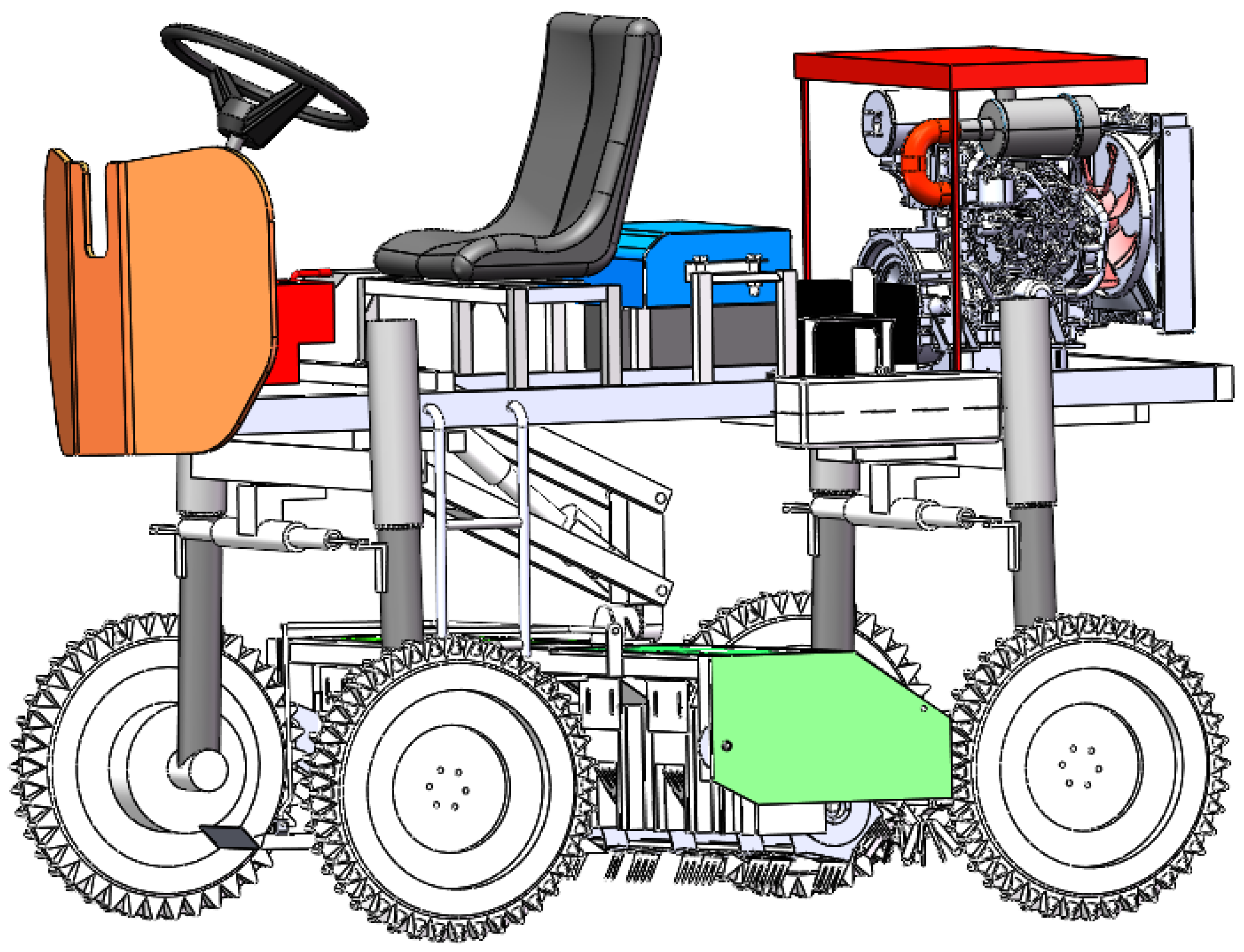
4.1.1. Chassis Modeling

The model of the paddy field weeder is built in SolidWorks 2021 software, the model is saved in SolidWorks in the *x_t format, and the import is selected in RecurDyn. A pavement model is created using the Track/LM toolkit. During the simulation, the mathematical model is automatically established in accordance with the relevant parameters and constraint input during the model establishment, and the data such as the displacement, speed, torque, and interaction between components can be outputted at any time for the hydraulic chassis [24,25] (Figure 3).

4.1.2. Paddy Field Pavement Modeling

The driving characteristics of the chassis are considerably influenced by the road condition simulation of paddy fields during weeder operation [26]. Thus, the modeling is performed using the ground module in the RecurDyn software. The damping coefficient is set to 0.25 and the dynamic friction coefficient is set to 0.3. The fixed constraint definition between the car body and the ground and the rotation constraint definition of the driving wheel are determined. In addition, it is necessary to establish the contact definition between the wheel and the ground. The flexible contact model used in this study is confirmed. Finally, the drive function of the driving wheel is defined, and the STEP function is studied in this paper. The driving wheel speed function is defined as STEP (Time, 0, 0, 2, 2.4), that is, within 2 s after starting, the angular speed of the driving wheel accelerates from 0 to 2.4 rad/s and then turns to uniform rotation.

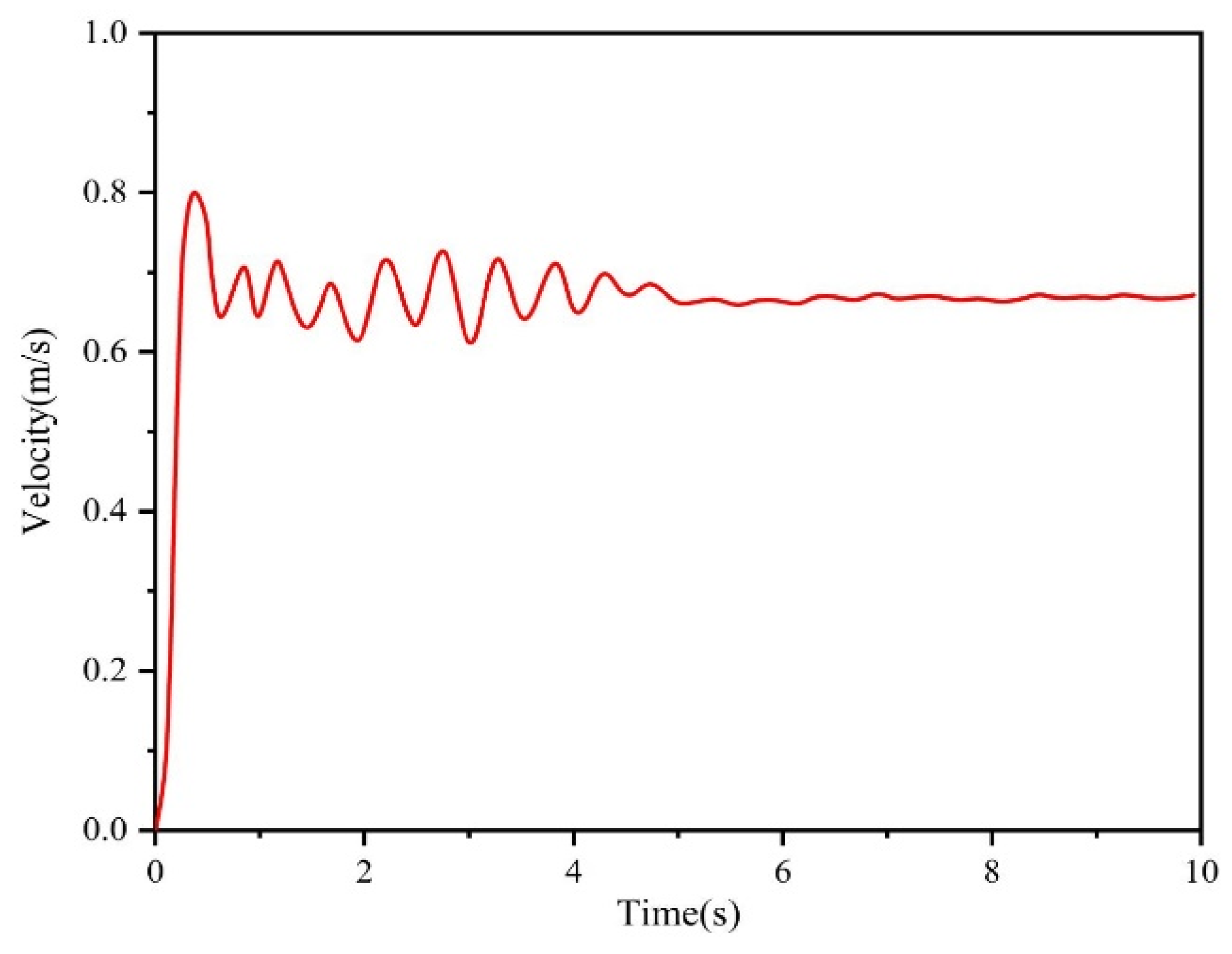
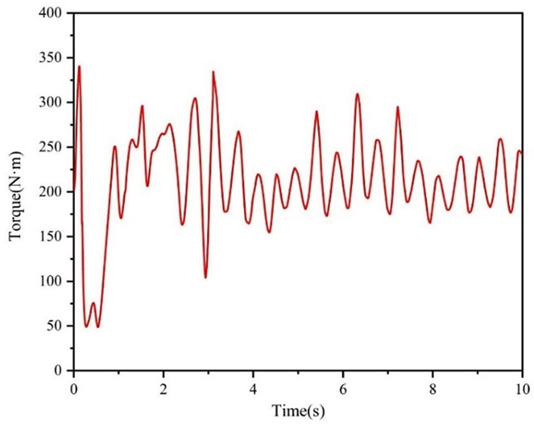
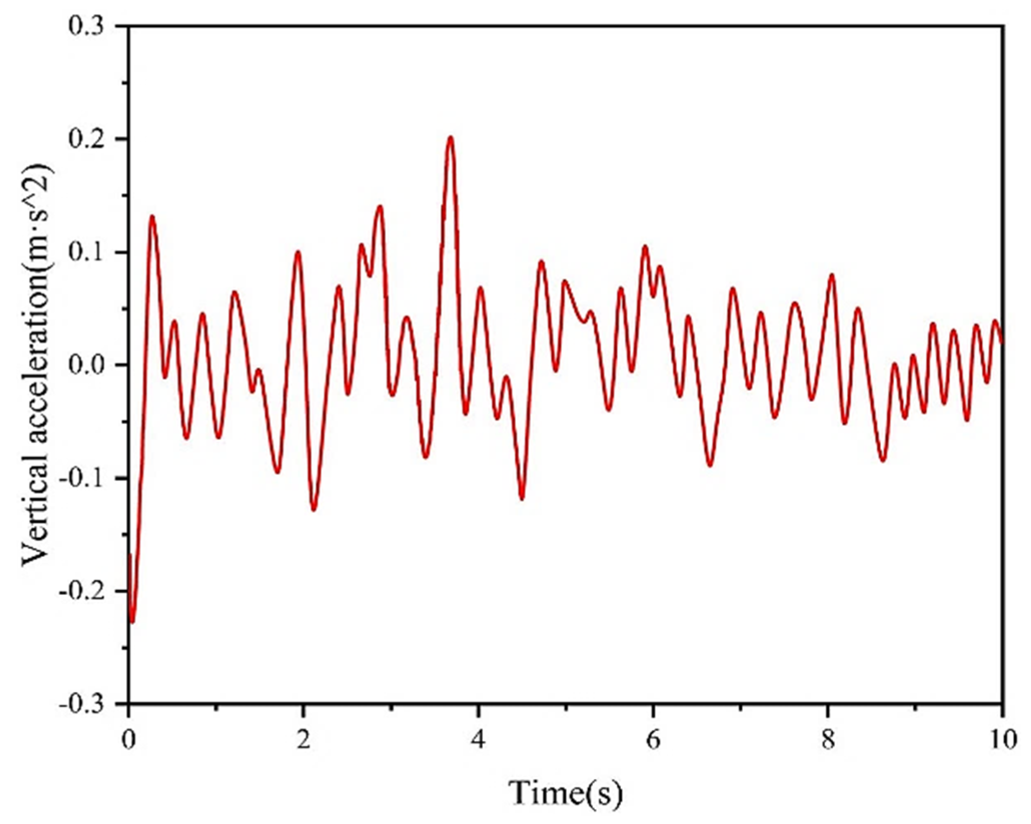
4.1.3. Analysis of Linear Driving Dynamics

When the horizontal velocity undergoes drastic changes, the chassis becomes susceptible to precarious phenomena, such as oscillation, trembling, or inclination. This inherent instability considerably elevates the likelihood of the chassis losing control when operating in agricultural lands, ultimately resulting in an undesirable overturning of the lawn mower. When encountering substantial lateral deviation, the chassis becomes predisposed to relinquish command over the intended driving trajectory, causing the weed removal device to deviate from the designated path and, in turn, augment the seedling pressure rate. This predicament becomes particularly pronounced in marshy paddy fields where the terrain is muddied, as the lawn mower becomes more vulnerable to irregular friction during operation, leading to fluctuations in the speed and continuous deviation from the desired driving path. As such, the smoothness and uninterrupted continuity of the horizontal velocity and lateral deviation variation curves emerge as pivotal factors for ensuring the steadfastness of the chassis during operation.

According to the actual driving condition of the chassis, the speed of the weeder in the paddy field is set at 0.7 m/s and then accelerated to the set speed within 5 s after starting, and the overall simulation time is 10 s. The horizontal velocity change curve of the center of mass is shown in Figure 4. After the hydraulic chassis is started, the set speed requirements are immediately reached, and the driving speed stabilizes after a fluctuation period. Large speed fluctuations before reaching stability may be due to the effects of the physical properties of the soil on the set pavement. The variation curve of the lateral deflection of the hydraulic chassis while driving on the paddy field road surface is shown in Figure 5. The deviation can verify the driving stability of the hydraulic chassis. This chassis is traveling at a speed of approximately 0.7 m/s on the paddy field road surface, the simulation time is 10 s, and the lateral deviation is approximately 13 cm. The deviation of the 100 m hydraulic chassis is approximately 1.86 m, and the deviation rate can be calculated as 1.86%. The actual driving condition is more complex than the simulation environment, which will be further verified by the following test.

In agricultural settings, the heightened peak torque facilitates swift acceleration and adept resistance management, thereby augmenting acceleration prowess and responsiveness, a pivotal aspect within such agricultural contexts. The torque change curve of the driving wheel during the hydraulic chassis driving at a speed of 0.7 m/s in the simulation environment is shown in Figure 6. The hydraulic chassis must overcome the starting acceleration and static friction force during its operation based on this figure. Moreover, the peak value of the required torque is large, and the peak value can reach 350 N·m. After 5 s, the chassis will enter a relatively stable driving state, and the small fluctuation in the stable working condition may be due to the existence of different degrees of subsidence on the paddy field road surface. The average torque is approximately 200 N·m.

The curve of the vertical acceleration change of the weeder while driving in the simulated environment is shown in Figure 7. Vertical acceleration refers to the acceleration of the vehicle in the vertical direction during driving, and the unit is m/s². The value range of vertical acceleration is also dependent on the specific application scenario and vehicle performance. The normal vertical acceleration is generally between 0.1 and 0.3 m/s² for ordinary passenger cars. Vertical acceleration can also exceed this range due to special circumstances, such as emergency braking, acceleration, and high-speed cornering. Vertical acceleration may even exceed 1 m/s² during hard braking or extreme driving [27,28]. The simulated speed change curve indicates that the speed of the weeder stabilizes after approximately 4 s, and the curve change amplitude of the vertical acceleration will also decrease. However, fluctuations will still exist within a certain range due to the inevitable discontinuity of the driving environment. The designed hydraulic chassis with good driving stability is observed in the simulation results.

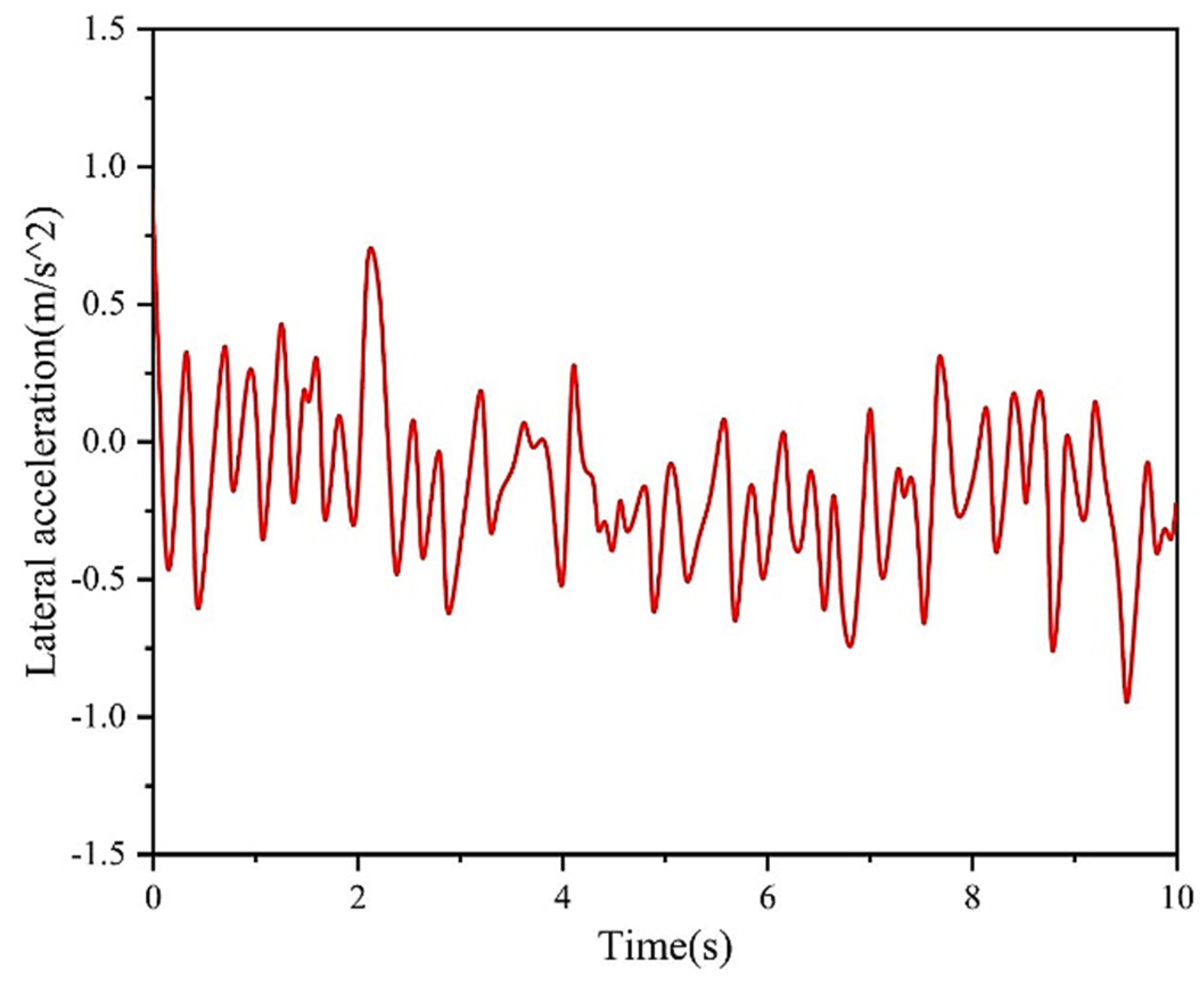
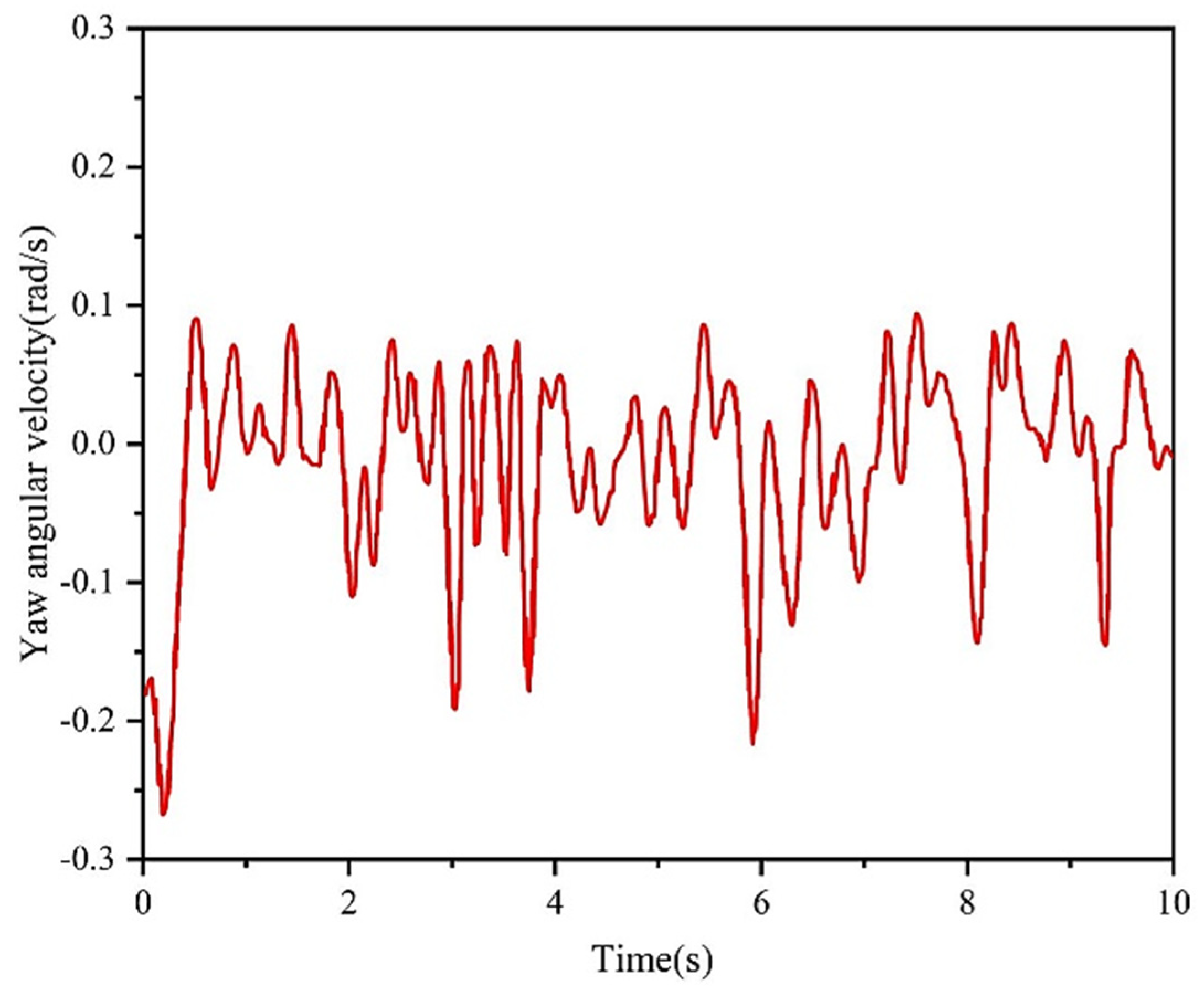
4.1.4. Steering Characteristic Analysis

Steering of the four-wheel-drive hydraulic chassis is realized through the differential speed of the left and right drive wheels [29]. The hydraulic flow rate of the hydraulic motor of each drive wheel is inputted through the steering cylinder regulation when the steering action is completed. Differential steering is rapidly achieved by the side with a large flow rate. The yaw velocity change curve of the weeder during its steering action with a simulation duration of 10 s in the simulation environment is shown in Figure 8. The yaw speed generally refers to the turning speed of the vehicle when driving on a curve (in rad/s). The average yaw speed can be between 0.5 and 1.5 rad/s for ordinary passenger cars. The yaw speed may also be high for vehicles such as high-performance racing cars, reaching more than 2 rad/s [30,31]. A large yaw velocity fluctuation of the weeder throughout the steering but within the normal range, a small yaw velocity, and hydraulic chassis control with superior stability are demonstrated by the simulation results [32].

The lateral acceleration change curve of the weeder during the steering action with a simulation duration of 10 s in the simulation environment is shown in Figure 9. The lateral acceleration is the ratio of the lateral force to the mass generated by the vehicle when driving on a curve, and the unit is m/s². The general lateral acceleration can be between 0.5 and 1.0 m/s² for ordinary passenger cars. The lateral acceleration may be higher for vehicles such as high-performance racing cars, reaching more than 1.5 m/s² [33,34]. The peak lateral acceleration reaches 0.75 m/s² during the simulation. If the lateral acceleration fluctuated frequently and exceeded the normal range, then the weeder would easily turn over when turning. The good steering stability of the designed hydraulic chassis is demonstrated by the simulation results.

4.2. Software Simulation of Chassis Walking Hydraulic System

4.2.1. Walking Hydraulic System Model

The simulation model of the walking hydraulic system is built in the Advanced Modeling Environment for performing Simulation of engineering systems (AMESim 2021.1) software according to the hydraulic schematic [35,36,37]. A hydraulic control component, a hydraulic actuator, a hydraulic auxiliary component, and a signal source are illustrated in Figure 10. An electromagnetic reversing valve, a relief valve, and a check valve comprise the hydraulic control components. A hydraulic cylinder and a hydraulic motor are both included in the hydraulic actuator. Meanwhile, an accumulator and a temperature regulator are included in the hydraulic auxiliary components. The electromagnetic reversing valve control signal is found in the signal source. The actual parameters are set for the hydraulic component module: the diesel engine speed is 3000 r/min, the dual pump displacement is 20 mL/r, and the hydraulic motor maximum displacement is 81.5 mL/r. The step signal for the process of stop, positive turn, and reverse is set by the electromagnetic reversing valve and is used to simulate the stopping forward and backward actions of the weeder.

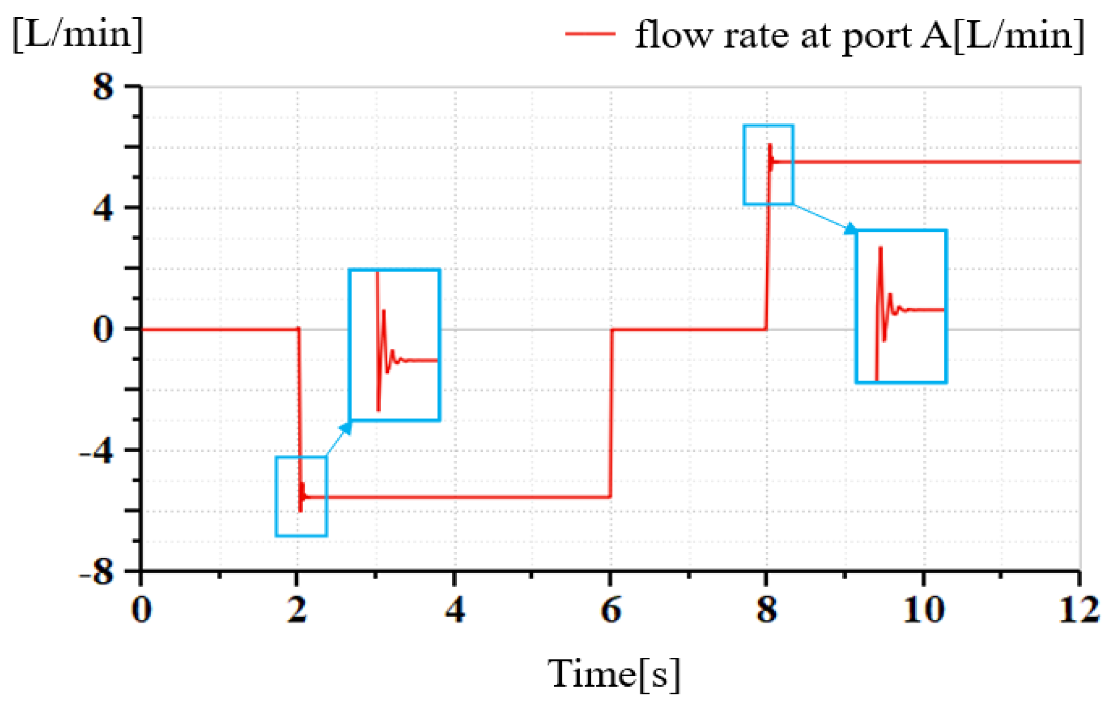
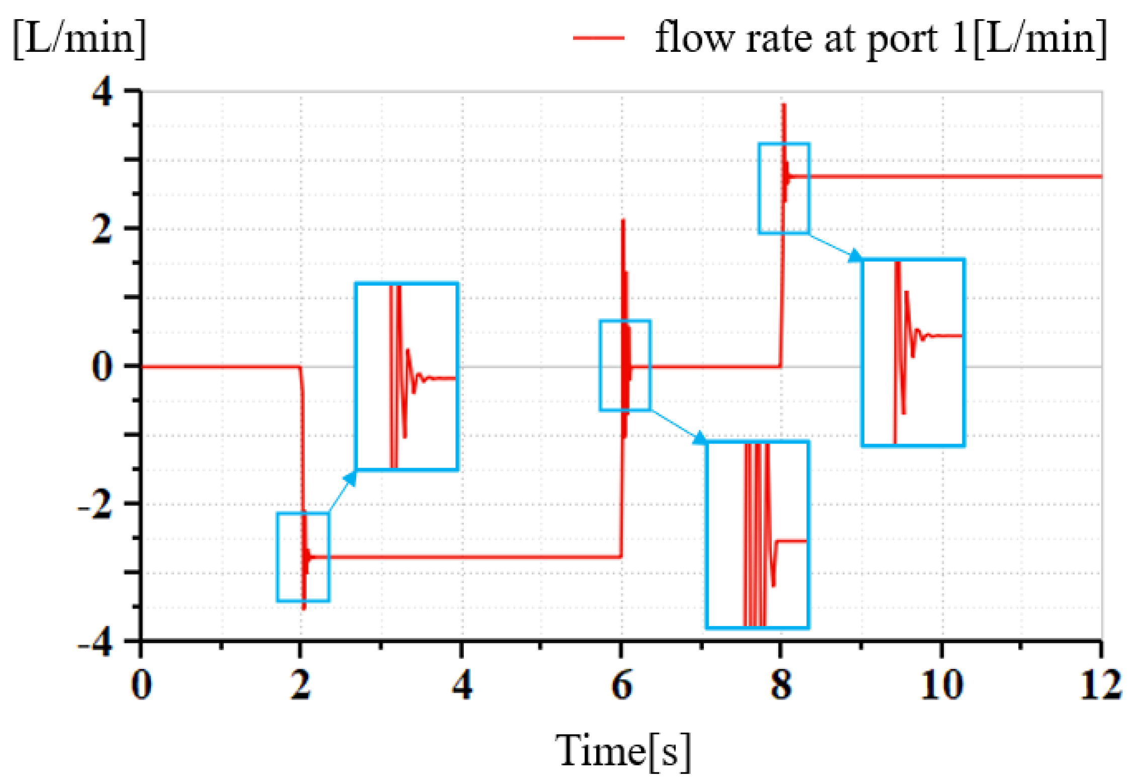
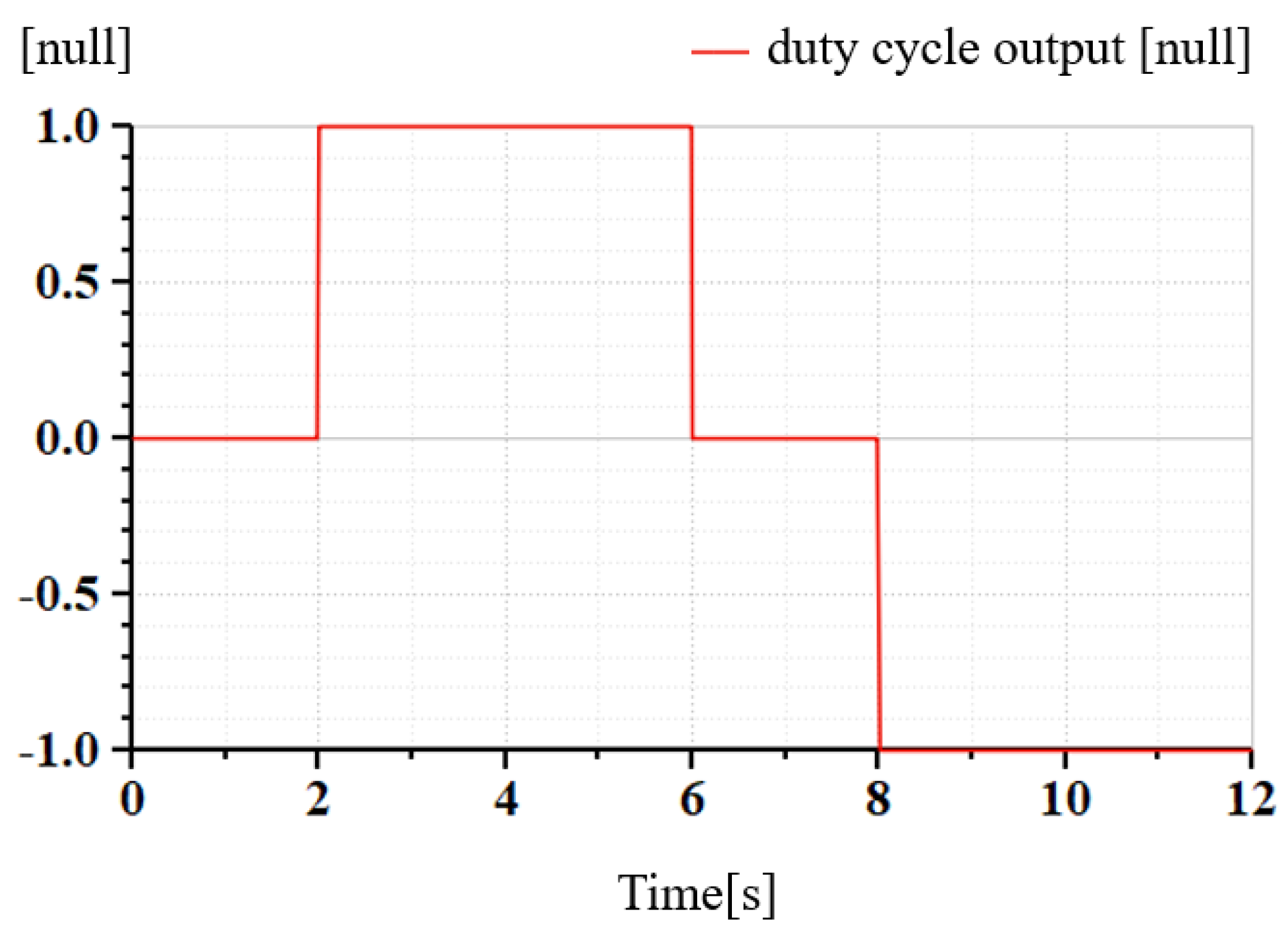
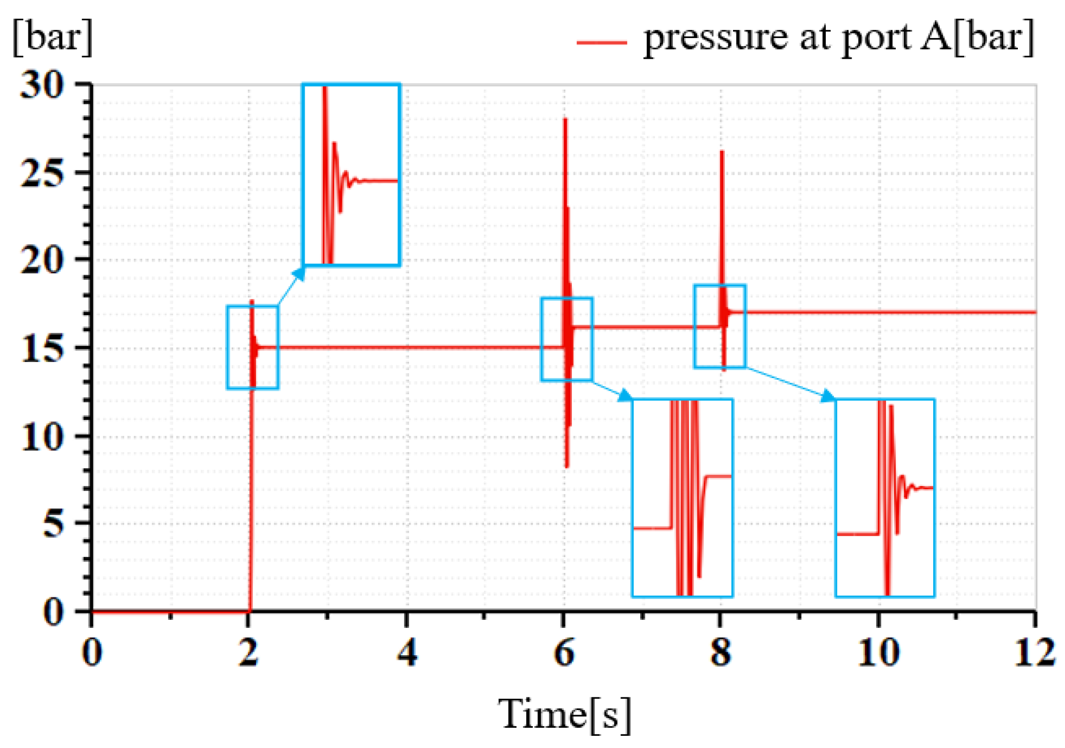
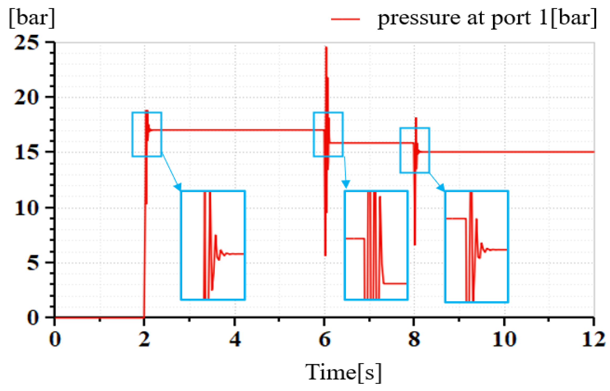
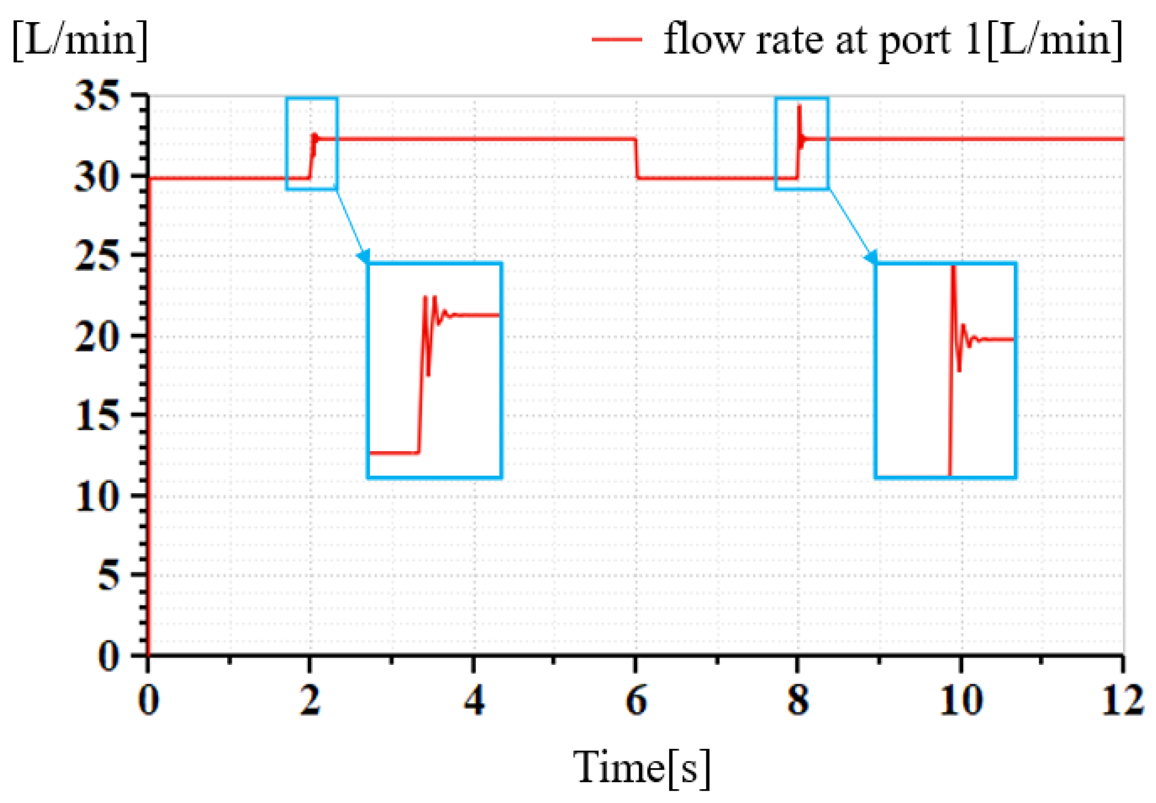
4.2.2. Travel Hydraulic Characteristics

The set step signals of the reversing valve are shown in Figure 11: stop 2 s, turn 4 s forward, stop 2 s, and reverse 4 s. The flow change curve of the reversing valve is shown in Figure 12. In the two positive and negative signal controls of 2–6 and 8–12 s, respectively, the flow rate of the reversing valve reaches 4.5 L/min (positive and negative represent the hydraulic oil flow direction), and the flow rate steadily changes. The peak pressure of the reversing valve reaches 2.5 MPa as shown in Figure 13, and the fluctuation mostly occurs at the start and stop time, which is relatively stable.

As shown in Figure 14, the chassis remains in a stagnant state at 0–2 s, the valve port of 2–6 s gradually increases, and the hydraulic motor flow rate rises to 2.5 L/min (positive or negative represents the hydraulic oil flow direction). When the chassis starts, the hydraulic oil that rushes into the motor will display an instantaneous impact, forming turbulence and resulting in a high flow rate. The flow rate stabilizes when the chassis travels at a constant speed. The sudden closure of the valve during the emergency stop also induces a large change in the impact of the hydraulic motor. The pressure characteristic curve of the traveling motor is shown in Figure 15. The pressure of the hydraulic motor remains stable at approximately 1.5 MPa under a constant chassis speed. As shown in Figure 16, the flow rate of the relief valve is maintained at approximately 30 L/min, effectively maintaining the safety of the hydraulic circuit.

5. Chassis Test

5.1. Linear Driving Offset Distance Test

5.1.1. Test Methods and Contents

The straightness test of the fully hydraulic-driven weeder was based on GB/T 15370.1-2012 [38] “General Technical conditions for Agricultural tractors Part 1: Wheeled tractors below 50 kW”, and the 100 m deviation of the tractor on the dry and flat slope (vertical and horizontal), which is not more than 1% of the road surface, should not exceed 6 m.

• Test site: Guang Ping District, Nanjing Agricultural University.
• Test equipment: A stopwatch (CASIO HS-70W accurate to 1/100 s), tape measure (STANLEY 30-455 with a range of 200 m and precision markings at the millimeter level), marking line, and hydraulic drive weeder.
• Test method: Prior to commencing the test, the hydraulic-driven weeder was brought to a complete stop. A starting point was designated, and chalk was used to mark this point on the ground, serving as the reference line. A vertical line was drawn from this starting point, and the end point was marked 100 m away in a straight line. Reference and vertical reference lines were established at the same horizontal position to ensure accurate measurement. The weeder was then driven from the starting point to the end point at a speed of 0.7 m/s, maintaining a consistent trajectory throughout the test. During the test, a stopwatch was employed to record the time taken by the weeder to traverse the 100 m distance. Upon the completion of each test run, a tape measure was used to measure the vertical deviation distance of the calibration line from the reference line. The recorded time and deviation data were meticulously documented for each of the five test runs, noting both positive and negative deviations to the left and right, respectively, for a comprehensive analysis.

The calculation formula for the deviation rate is as follows:

$$\beta =\frac{∆\gamma }{\gamma }\times 100\%$$

(9)

where $\beta$ is the rate of deflection, $∆\gamma$ is the offset distance (m), and $\gamma$ is the designated driving distance (m).

5.1.2. Test Results and Analysis

The deviation test diagram is shown in Figure 17. The full hydraulic track chassis passed the starting point at the maximum speed during each test and drove at a constant speed to the end. The test deviation rate results are presented in the

Table 5. Test results of deviation rate.

Pilot Project	Data
Offset distance/m	2.84
	2.54
	2.23
	2.97
	2.47
Average deviation/m	2.61

.

An analysis of the test results shows a positive deviation rate, left deviation of the vehicle, and an average deviation rate of 2.61%, which is larger than the deviation rate of 1.86% obtained in the simulation analysis. The actual deviation rate of the actual road surface will be larger than the simulation value due to the differences in the hydraulic components and installation and the complicated actual road conditions. However, the deviation amount remained within the permissible range, thereby satisfying the design requirements.

5.2. Slip Rate Test Experiment

5.2.1. Test Methods and Contents

The loop flow calculation of the full hydraulic drive system was realized by obtaining the slip rate of the weeder operating in the paddy field. Different from the hard pavement with good adhesion conditions, the stress situation of paddy field pavement is complicated and difficult to estimate using an empirical formula. A test of the paddy field slip rate with the weeder was conducted to obtain accurate slip rate data.

• Test site: The rice–wheat Science and Technology Demonstration Center, Jintan District, Changzhou City, Jiangsu Province, with a subtropical monsoon climate, four distinct seasons, abundant precipitation, and mild climate, suitable for rice growth.
• Test equipment: A tape measure (STANLEY 30-455 with a range of 200 m and precision markings at the millimeter level), revolution counter (DTI ±0.1 revolution), and hydraulic drive weeder.
• Experimental sample field: A rice–wheat continuous cropping field, wherein the land uniformity of the experimental area is consistent.
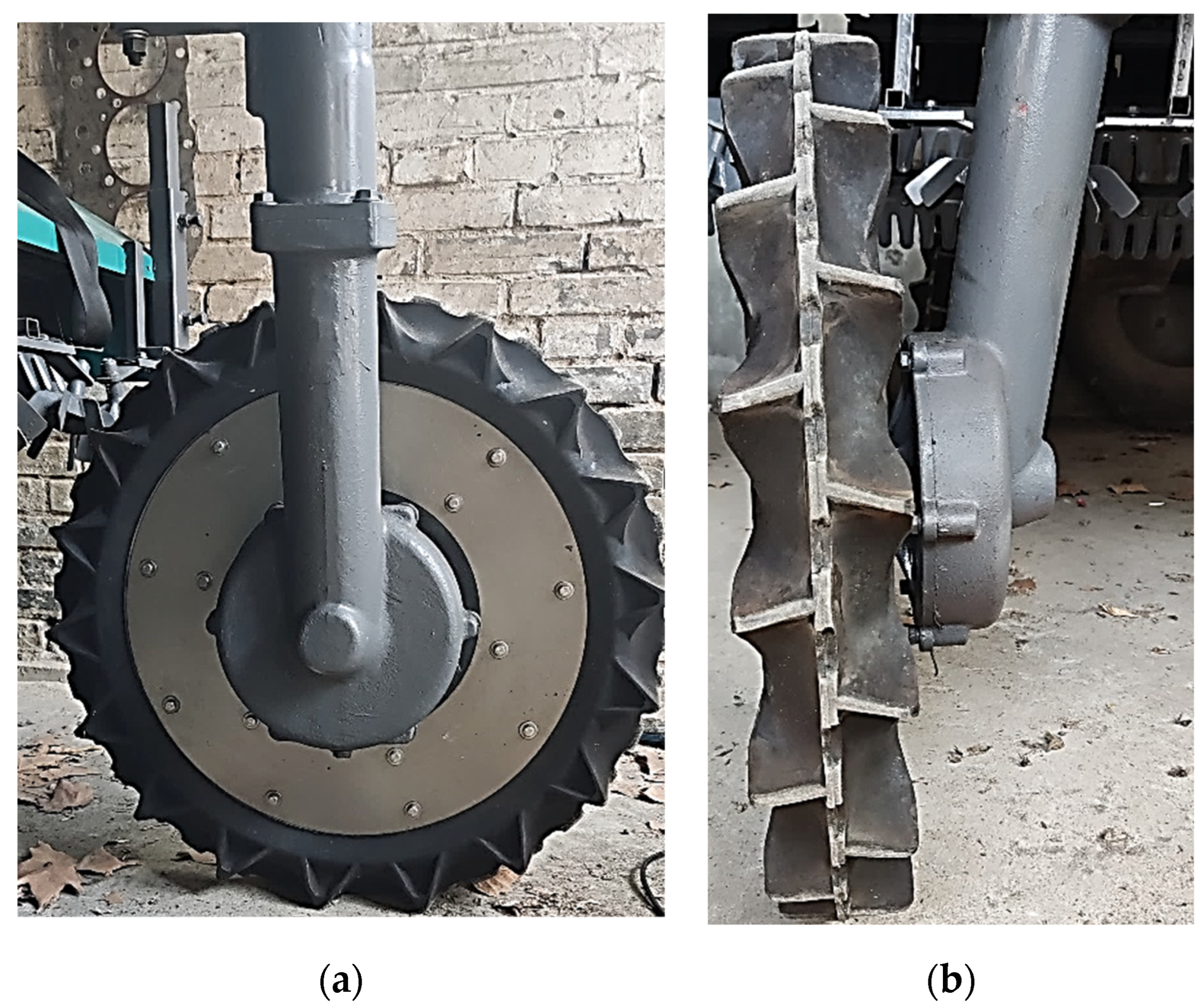
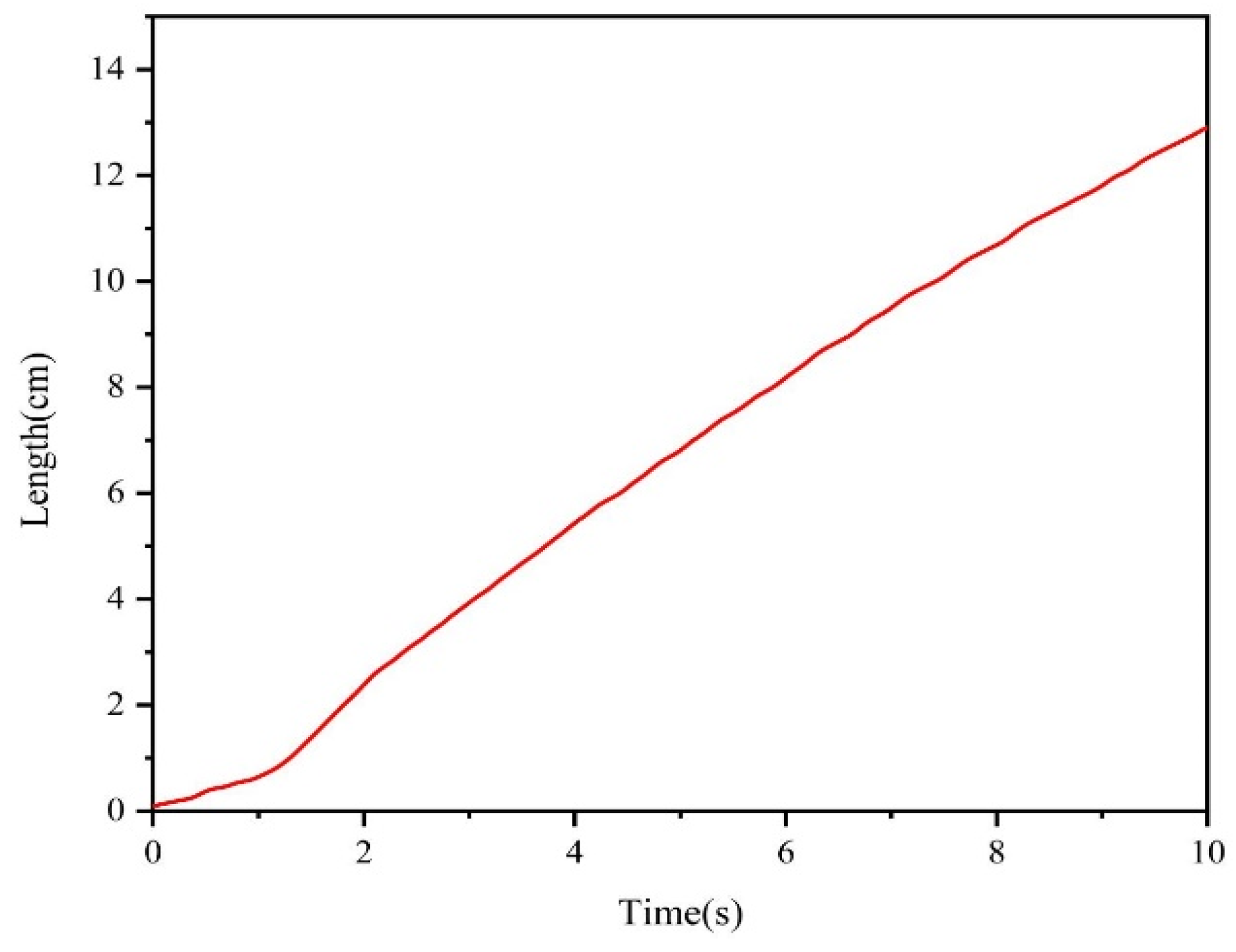
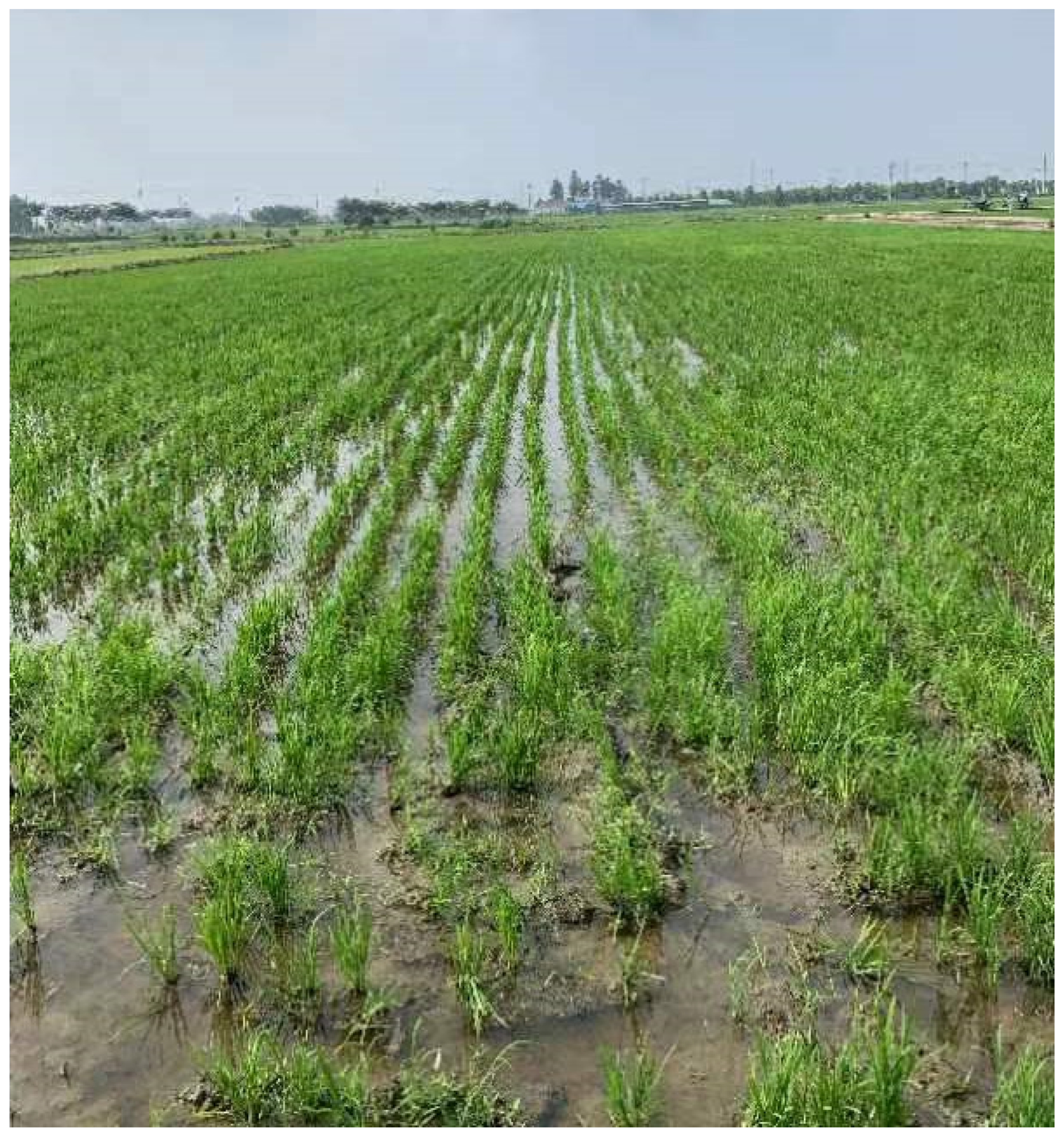
• Test methods: The driving wheel of the weeder was selected as the experimental observation object, and the theoretical driving linear distance of the weeder’s driving wheel rotating 10 turns was calculated. The testing speed was 0.7 m/s. The actual driving distance was then measured with a meter ruler to calculate its slip rate. The revolution counter was used to measure the rotation times of the driving wheel of the weeder. To reduce the experimental errors, the average of three measurements was taken as the final result (Figure 18 and Figure 19).

5.2.2. Test Results and Analysis

The test data are shown in

Table 6. Test data.

Group Number	Actual Travel Distance/m	Theoretical Travel Distance/m	Slippage Rate/%
1	25.36	26.70	5.01
2	25.83	26.70	3.27
3	26.03	26.70	2.49
Average value	37.14	26.70	3.59

.

Table 6 shows that under the precondition of the weeder operating at a speed of 0.7 m/s, the maximum and minimum slip rates of the weeder traveling in a straight line obtained by the test are 5.01% and 2.49%, respectively, which may be attributed to the poor bearing capacity of the paddy field and the complex environment. The average slip rate is 3.59%. In the previous research on the hydraulic chassis of a plant protection machine, when driven at speeds of 0.83 and 1.67 m/s, the average slip rates were 3.79% and 6.17%, respectively, which demonstrates a similar effect to that observed in this study [39]. However, it is worth noting that the working environment of the weed removal machine described in this article occurs approximately 15 days after transplanting, during which the soil moisture content is high. This high moisture content poses challenges in controlling the precision of the slip rate, adding complexity to the operational dynamics of the machine. Therefore, the herbicide chassis designed in this article effectively solves the problem of a high slip rate in rice fields.

6. Conclusions

(1)

The horizontal speed of the hydraulic chassis of the designed weeder fluctuated and stabilized at 0.7 m/s. The torque of the driving wheel stabilized at approximately 200 N·m, and the peak vertical acceleration reached 0.2 m/s². The yaw speed and lateral acceleration of the chassis also fluctuated within the normal range during steering, and the driving remained relatively stable.

(2)

When the hydraulic chassis of the designed weeder was running, the flow rate of the reversing valve reached 4.5 L/min, and the peak flow of the hydraulic motor was 2.5 L/min. The selected hydraulic components addressed the requirements of the working conditions, the hydraulic motor flow and pressure changes were in a reasonable range, and the hydraulic system oil supply flow remained stable.

(3)

The drift rate of the weeder was 2.61%, and the average slip rate of the paddy field was 3.59% under the precondition of the weeder operating at a speed of 0.7 m/s. Thus, the future design of hydraulic systems under specific working conditions in actual production work can be guided by this study.

Moreover, future studies could focus on implementing advanced control algorithms or adaptive mechanisms to address drift and slip rates more effectively. By incorporating real-time feedback and predictive analytics, we can strive to minimize these undesirable phenomena and improve the overall precision and reliability of the weeder in paddy field environments.

References

1. Bin Rahman, A.N.M.R.; Zhang, J. Trends in rice research: 2030 and beyond. Food Energy Secur. 2023, 12, e390. [Google Scholar] [CrossRef]
2. Farooq, M.; Siddique, K.H.; Rehman, H.; Aziz, T.; Lee, D.-J.; Wahid, A. Rice direct seeding: Experiences, challenges and opportunities. Soil Tillage Res. 2011, 111, 87–98. [Google Scholar] [CrossRef]
3. Monteiro, A.; Santos, S. Sustainable Approach to Weed Management: The Role of Precision Weed Management. Agronomy 2022, 12, 118. [Google Scholar] [CrossRef]
4. Raza, A.; Ali, H.H.; Zaheer, M.S.; Iqbal, J.; Seleiman, M.F.; Sattar, J.; Ali, B.; Khan, S.; Arjumend, T.; Chauhan, B.S. Bio-ecology and the management of Chenopodium murale L.: A problematic weed in Asia. Crop Prot. 2023, 172, 106332. [Google Scholar] [CrossRef]
5. Westwood, J.H.; Charudattan, R.; Duke, S.O.; Fennimore, S.A.; Marrone, P.; Slaughter, D.C.; Swanton, C.; Zollinger, R. Weed Management in 2050: Perspectives on the Future of Weed Science. Weed Sci. 2018, 66, 275–285. [Google Scholar] [CrossRef]
6. Holt, J.S. Impact of Weed Control on Weeds: New Problems and Research Needs. Weed Technol. 1994, 8, 400–402. [Google Scholar] [CrossRef]
7. Griepentrog, H.W.; Gulhom-Hansen, T.; Nielsen, J. First field results from intra-row rotor weeding. In Proceedings of the 7th European Weed Research Society Workshop on Physical and Cultural Weed Control, Salem, Germany, 11–14 March 2007. [Google Scholar]
8. Tillett, N.; Hague, T.; Grundy, A.; Dedousis, A. Mechanical within-row weed control for transplanted crops using computer vision. Biosyst. Eng. 2008, 99, 171–178. [Google Scholar] [CrossRef]
9. Shoji, K.; Itoh, K.; Kawahara, F.; Yoshida, Y.; Yamamoto, Y.; Sudo, K.-I. Micro-elevations in paddy fields affect the efficacy of mechanical weeding: Evaluation of weeding machines to control Monochoria vaginalisin herbicide-free farming. Weed Biol. Manag. 2013, 13, 45–52. [Google Scholar] [CrossRef]
10. Jinw, W. Design of organic rice cultivation weeding. J. Northeast. Agric. Univ. 2013, 44, 107–112. [Google Scholar]
11. Qi, L.; Ma, X.; Tan, Z.; Tan, Y.; Qiu, Q.; Yang, C.; Zhang, W. Development and experiment of marching-type inter-cultivation weeder for paddy. Trans. Chin. Soc. Agric. Eng. (Trans. CSAE) 2012, 28, 31–35. [Google Scholar]
12. Matsuda, Y.; Kakutani, K.; Toyoda, H. Unattended Electric Weeder (UEW): A Novel Approach to Control Floor Weeds in Orchard Nurseries. Agronomy 2023, 13, 1954. [Google Scholar] [CrossRef]
13. Wu, C.; Zhang, M.; Jin, C.; Tu, A.; Lu, Y.; Xiao, T. Design and experiment of 2BYS-6 type paddy weeding-cultivating machine. Nongye Jixie Xuebao (Trans. Chin. Soc. Agric. Mach.) 2009, 40, 51–54. [Google Scholar]
14. Qi, L.; Zhao, L.; Ma, X.; Cui, H.; Zheng, W.; Lu, Y. Design and test of 3GY-1920 wide-swath type weeding-cultivating machine for paddy. Nongye Gongcheng Xuebao/Trans. Chin. Soc. Agric. Eng. 2017, 33, 47–55. [Google Scholar]
15. Sanchez, J.; Gallandt, E.R. Functionality and efficacy of Franklin Robotics’ Tertill™ robotic weeder. Weed Technol. 2021, 35, 166–170. [Google Scholar] [CrossRef]
16. Nissing, D.; Gessat, J.; Bitzer, T.; Seewald, A. Hydraulic chassis systems with electrically powered hydraulic steering and active roll control. ATZ Worldw. 2007, 109, 11–15. [Google Scholar] [CrossRef]
17. Han, X.; Su, W.; Zhao, H.; Zheng, Y.; Hu, Q.; Wang, C. The applications of energy regeneration and conversion technologies based on hydraulic transmission systems: A review. Energy Convers. Manag. 2020, 205, 112413. [Google Scholar]
18. Rossetti, A.; Macor, A. Continuous formulation of the layout of a hydromechanical transmission. Mech. Mach. Theory 2019, 133, 545–558. [Google Scholar] [CrossRef]
19. Triet, H.H.; Ahn, K.K. Comparison and assessment of a hydraulic energy-saving system for hydrostatic drives. Proc. Inst. Mech. Eng. Part I J. Syst. Control. Eng. 2011, 225, 21–34. [Google Scholar] [CrossRef]
20. Comellas, M.; Pijuan, J.; Nogués, M.; Roca, J. Efficiency analysis of a multiple axle vehicle with hydrostatic transmission overcoming obstacles. Veh. Syst. Dyn. 2018, 56, 55–77. [Google Scholar] [CrossRef]
21. Morera-Torres, E.; Ocampo-Martinez, C.; Bianchi, F.D. Experimental Modelling and Optimal Torque Vectoring Control for 4WD Vehicles. IEEE Trans. Veh. Technol. 2022, 71, 4922–4932. [Google Scholar] [CrossRef]
22. Qi, X.; Shang, Y.; Ding, Z.; Wei, W. Particularities and research progress of the cutting machinability of wood-plastic composites. Mater. Today Commun. 2023, 37, 106924. [Google Scholar] [CrossRef]
23. Baek, S.-Y.; Baek, S.-M.; Jeon, H.-H.; Kim, W.-S.; Kim, Y.-S.; Sim, T.-Y.; Choi, K.-H.; Hong, S.-J.; Kim, H.; Kim, Y.-J. Traction Performance Evaluation of the Electric All-Wheel-Drive Tractor. Sensors 2022, 22, 785. [Google Scholar] [CrossRef] [PubMed]
24. Yun, S.; Lee, W.; Park, J.; Guak, K. Development of a Virtual Environment Co-Simulation Platform for Evaluating Dynamic Characteristics of Self-Balancing Personal Mobility. IEEE Trans. Veh. Technol. 2021, 70, 2969–2978. [Google Scholar] [CrossRef]
25. Tang, S.; Guo, Z.; Wang, G.; Wang, X. Comparative Performance Analysis of Different Travelling Mechanisms Based on RecurDyn. IOP Conf. Ser. Mater. Sci. Eng. 2020, 782, 42059. [Google Scholar] [CrossRef]
26. Li, Y.; Dai, S.; Zheng, Y.; Tian, F.; Yan, X. Modeling and Kinematics Simulation of a Mecanum Wheel Platform in RecurDyn. J. Robot. 2018, 2018, 9373580. [Google Scholar] [CrossRef]
27. Santos, M.; López, R.; de la Cruz, J.M. Fuzzy control of the vertical acceleration of fast ferries. Control Eng. Pract. 2005, 13, 305–313. [Google Scholar] [CrossRef]
28. Zong, Z.; Sun, Y.; Jiang, Y. Experimental study of controlled T-foil for vertical acceleration reduction of a trimaran. J. Mar. Sci. Technol. 2019, 24, 553–564. [Google Scholar] [CrossRef]
29. Cakici, F.; Yazici, H.; Alkan, A.D. Optimal control design for reducing vertical acceleration of a motor yacht form. Ocean Eng. 2018, 169, 636–650. [Google Scholar] [CrossRef]
30. Ricco, M.; Zanchetta, M.; Rizzo, G.C.; Tavernini, D.; Sorniotti, A.; Chatzikomis, C.; Velardocchia, M.; Geraerts, M.; Dhaens, M. On the Design of Yaw Rate Control via Variable Front-to-Total Anti-Roll Moment Distribution. IEEE Trans. Veh. Technol. 2020, 69, 1388–1403. [Google Scholar] [CrossRef]
31. Chen, T.; Xu, X.; Chen, L.; Jiang, H.; Cai, Y.; Li, Y. Estimation of longitudinal force, lateral vehicle speed and yaw rate for four-wheel independent driven electric vehicles. Mech. Syst. Signal Process. 2018, 101, 377–388. [Google Scholar] [CrossRef]
32. Marino, R.; Scalzi, S. Asymptotic sideslip angle and yaw rate decoupling control in four-wheel steering vehicles. Veh. Syst. Dyn. 2010, 48, 999–1019. [Google Scholar] [CrossRef]
33. Jagelčák, J.; Gnap, J.; Kostrzewski, M.; Kuba, O.; Frnda, J. Calculation of an Average Vehicle’s Sideways Acceleration on Small Roundabouts. Sensors 2022, 22, 4978. [Google Scholar] [CrossRef] [PubMed]
34. Takahashi, T. The influence of tyre transient side force properties on vehicle lateral acceleration for a time-varying vertical force. Veh. Syst. Dyn. 2018, 56, 734–752. [Google Scholar] [CrossRef]
35. Lin, T.; Wang, L.; Huang, W.; Ren, H.; Fu, S.; Chen, Q. Performance analysis of an automatic idle speed control system with a hydraulic accumulator for pure electric construction machinery. Autom. Constr. 2017, 84, 184–194. [Google Scholar] [CrossRef]
36. Kim, J.; Lee, J.; Kim, K. Numerical study on the effects of fuel viscosity and density on the injection rate performance of a solenoid diesel injector based on AMESim. Fuel 2019, 256, 115912. [Google Scholar] [CrossRef]
37. Li, H.; Li, S.; Sun, W.; Wang, L.; Lv, D. The optimum matching control and dynamic analysis for air suspension of multi-axle vehicles with anti-roll hydraulically interconnected system. Mech. Syst. Signal Process. 2020, 139, 106605. [Google Scholar] [CrossRef]
38. GB/T 15370.1-2012; General Requirement of Agricultural Tractors—Part 1: Under 50 kW Wheeled Tractors. National Standards of People’s Republic of China: Beijing, China, 2012.
39. Zhang, C.; Li, C.; Zhao, C.; Li, L.; Gao, G.; Chen, X. Design of Hydrostatic Chassis Drive System for Large Plant Protection Machine. Agriculture 2022, 12, 1118. [Google Scholar] [CrossRef]
Figure 1. Physical photo of the chassis of the paddy field weeder: 1. steering column; 2. hydraulic lifting control device; 3. battery pack; 4. hydraulic oil tank; 5. steering machine; 6. hydraulic pipe; 7. diverter valve; 8. hydraulic motor; 9. chassis steel frame; and 10. duplex pump.
Agriculture 14 00595 g001
Figure 2. Schematic of hydraulic system: 1. check valve; 2. hydraulic motor; 3. two-position two-way solenoid valve; 4. three-position four-way solenoid directional valve; 5. two-position three-way reversing valve; 6. manometer; 7. energy accumulator; 8. cylinder; 9. engine; 10. double pump; 11. level gauge; 12. thermometer; 13. temperature regulator; and 14. relief valve.
Agriculture 14 00595 g002
Figure 3. Modeling diagram of hydraulic-driven weeder.
Agriculture 14 00595 g003
Figure 4. Horizontal velocity change curve of chassis center of mass.
Agriculture 14 00595 g004
Figure 5. Curve of lateral deviation.
Agriculture 14 00595 g005
Figure 6. Torque change curve of driving wheel.
Agriculture 14 00595 g006
Figure 7. Curve of vertical acceleration.
Agriculture 14 00595 g007
Figure 8. Curve of yaw velocity.
Agriculture 14 00595 g008
Figure 9. Curve of lateral acceleration.
Agriculture 14 00595 g009
Figure 10. Hydraulic system simulation modeling diagram.
Agriculture 14 00595 g010
Figure 11. Step signal of reversing valve.
Agriculture 14 00595 g011
Figure 12. Flow curve of reversing valve.
Agriculture 14 00595 g012
Figure 13. Pressure change curve of reversing valve.
Agriculture 14 00595 g013
Figure 14. Flow curve of hydraulic motor.
Agriculture 14 00595 g014
Figure 15. Pressure change curve of hydraulic motor.
Agriculture 14 00595 g015
Figure 16. Flow change curve of relief valve.
Agriculture 14 00595 g016
Figure 17. Deviation test diagram.
Agriculture 14 00595 g017
Figure 18. Driving wheel style and tire pattern: (a) driving wheel style and (b) tire pattern.
Agriculture 14 00595 g018
Figure 19. Working environment of paddy field.
Agriculture 14 00595 g019