AI-Driven Model Prediction of Motions and Mooring Loads of a Spar Floating Wind Turbine in Waves and Wind

Abstract

This paper describes a Long Short-Term Memory (LSTM) neural network model used to simulate the dynamics of the OC3 reference design of a Floating Offshore Wind Turbine (FOWT) spar unit. It crafts an advanced neural network with an encoder–decoder architecture capable of predicting the spar’s motion and fairlead tensions time series. These predictions are based on wind and wave excitations across various operational and extreme conditions. The LSTM network, trained on an extensive dataset from over 300 fully coupled simulation scenarios using OpenFAST, ensures a robust framework that captures the complex dynamics of a floating platform under diverse environmental scenarios. This framework’s effectiveness is further verified by thoroughly evaluating the model’s performance, leveraging comparative statistics and accuracy assessments to highlight its reliability. This methodology contributes to substantial reductions in computational time. While this research provides insights that facilitate the design process of offshore wind turbines, its primary aim is to introduce a new predictive approach, marking a step forward in the quest for more efficient and dependable renewable energy solutions.

1. Introduction

The search for sustainable and reliable energy solutions has increasingly turned toward the oceans, with Floating Offshore Wind Turbines (FOWTs) emerging as pivotal technologies in harnessing marine wind resources [1]. The complexity and stochastic nature of marine environments, characterized by the dynamic interactions of waves, wind, and currents, presents significant challenges in the design and operation of FOWTs. Understanding the hydrodynamic responses of these structures, especially under extreme conditions, is crucial for their safety, efficiency, and longevity. Engineers and designers frequently conduct evaluations and forecasting using various [2] numerical time-domain coupled analyses. In this context, OpenFAST has emerged as an integrated tool, capturing the complete behavior of wind turbine systems—including the turbine, support structure, mooring lines, and the marine environment—to facilitate a comprehensive understanding of system dynamics [3]. While foundational, these studies require large computational resources and face challenges in accurately predicting FOWTs’ non-linear responses to varied sea states, requiring extensive simulations and tuning to validate them.

To obtain the dynamic response of FOWT at a reasonable time, some researchers have improved the time-domain coupling analysis methods. Many of these approaches employ a decoupled analysis in the time domain, treating the platform’s mooring lines as quasi-static springs, while enhancing the model by incorporating the dynamic effects of the lines through equivalent linear damping and inertia coefficients [4,5]. However, these approaches have some inherent limitations, as drag-induced damping is non-linear and thus dependent on the amplitude of the oscillation. More recently, Low and Langley [6] introduced a hybrid method that simulates low-frequency motion in the time domain and wave frequency motion in the frequency domain, thereby reducing the computational load and enhancing the efficiency of time-domain evaluation methods. Nevertheless, the methods’ computational demand, though reduced, still poses challenges, highlighting an ongoing quest for more efficient predictive models.

Parallel to these developments, the field of artificial intelligence (AI), particularly data-driven neural network models (ANN), has shown promise in capturing temporal dependencies and complex patterns in sequential data while reducing computational time. Many scholars and researchers have considered selecting the appropriate model to resolve issues related to time series prediction problems [7]. Feedforward Neural Networks (FNNs) are broadly used in many time series forecasting applications [8,9,10], as well as for the optimization of the mooring lines of FOWT [11,12] to reduce their costs. Nevertheless, while effective for certain tasks, these simple models often fall short when handling the non-linearity and long-term dependencies inherent in complex time series data. This limitation has led to the exploration and adoption of more advanced neural network architectures, such as Recurrent Neural Networks (RNN), proposed in the 1980s, which are capable of storing information for a long time in hidden states [13]. RNNs achieve this by using loops within the network structure, allowing information to be passed from one step of the network to the next. This looping mechanism enables the network to maintain a form of memory, capturing dependencies across different time steps. In particular, one of the self-looping-based RNNs, the Long Short-Term Memory (LSTM) [14,15], has gained significant attention for its ability to understand long-term sequential dependencies, making them exceptionally suitable for forecasting tasks. Consequently, LSTMs present a groundbreaking methodology for predicting seakeeping dynamics, leveraging large response datasets.

The ability of ANN models to learn complex long-term dependencies at low computational cost suggests a potential paradigm shift in how to obtain the dynamic response of FOWTs. It aligns with the recent research of Bjørni et al. [16], where they explored machine learning’s impact on predicting spar floating wind turbine mooring tensions using motion time series as inputs, finding generally strong correlations, except in extreme sea states. Silva and Maki [17] crafted an LSTM neural network for simulating a ship’s six degrees of freedom (DoF) motions at 20 knots in irregular seas, evaluating model accuracy against wave inputs and the training data quantity. Lee et al. [18] presented novel integrated architectures, combining an LSTM encoder and decoder with a convolutional neural network. These have been utilized to forecast ship motion, taking the encoded initial state vector and anticipated ocean wave field information around a vessel. Most recently, Park et al. [19] proposed a novel methodology using FNN to predict the occurrence of green water events in terms of relative wave motions around the hull. In this work, the authors compared the prediction performance between the ANN-based models and the linear model for the peak value of relative wave motion, in which the ANN-based model significantly reduced the prediction error of the linear prediction model.

Building on these advancements and addressing the challenges in sequence learning for FOWT platforms, this study introduces a novel LSTM-based neural network model, implemented using PyTorch (version 2.3.0), that transcends traditional methodologies in simulating the dynamic responses of FOWTs. It bridges the existing gap in the literature regarding the application of AI techniques to infer time-domain responses for FOWTs, using as input operational and severe sea states and wind conditions, leveraging a comprehensive dataset derived from over 300 fully coupled simulations using OpenFAST for the time domain (TD) and ANSYS AQWA for the frequency domain (FD) of the OC3 reference design [20]. The model developed not only forecasts the motion time series, but also extends its predictive power to fairlead tensions under operational and extreme wind and wave conditions. This approach promises to accelerate the prediction process of FOWT dynamics while revolutionizing real-time monitoring and control strategies, thereby improving offshore wind energy systems’ design and operational efficiency. Through rigorous validation and performance evaluation, our research sets a new benchmark in seakeeping analyses in marine sciences, paving the way for more resilient and efficient renewable energy solutions.

This paper is organized as follows: Section 2 defines the case study, Section 3 describes the numerical simulation model, and Section 4 describes the neural network setup applied in the present research. Section 5 presents the results obtained and their evaluation. Finally, in Section 6, some conclusions and future lines of works are discussed.

2. Case Study

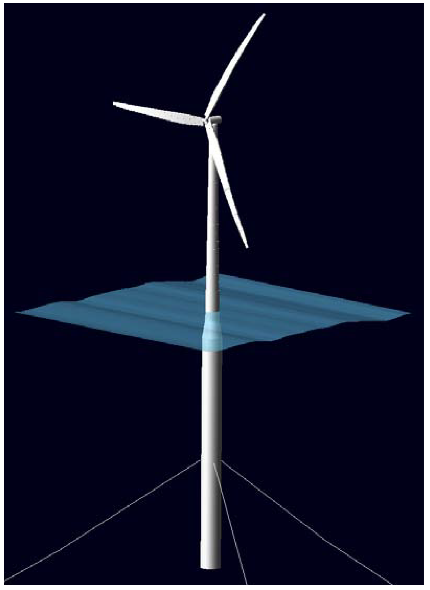
2.1. Floating Wind Turbine Model

The OC3-Hywind model [20] is a reference wind turbine that comprises a spar-type floating wind turbine (FWT) of 5 megawatts, anchored by three catenary mooring lines. This concept has been chosen in the current work as proof of concept due to its extensive validation of both experimental [21,22] and numerical data [20,23], providing a robust foundation for comparative analysis of the performance and accuracy of the numerical simulations carried out in the present study.

The draft of the platform is 120 m, and between 4 m and 12 m below the sea water level (SWL) extends a linearly tapering conical transition region that connects two cylinder diameters of 9.4 m below the taper with a slender one of 6.5 m. Figure 1 illustrates the concept. More details on the platform’s inertia, mass, and mooring properties can be found in

Table 1. Summary of OC3-Hywind spar properties.

Properties	Value
Total Platform Mass	7,466,330 kg
Vertical Position of Center of Gravity (Below SWL)	89.9 m
Platform Roll Inertia (about Center of Gravity)	4,229,230,000 $\mathrm{kg}·{\mathrm{m}}^2$
Platform Pitch Inertia (about Center of Gravity)	4,229,230,000 $\mathrm{kg}·{\mathrm{m}}^2$
Platform Yaw Inertia (about Center of Gravity)	164,230,000 $\mathrm{kg}·{\mathrm{m}}^2$
Number of Mooring Lines	3
Angle Between Adjacent Lines	120°
Unstretched Mooring Line Length	902.2 m
Equivalent Mooring Line Weight in Water	698.09 N/m
Equivalent Mooring Line Extensional Stiffness	384,243,000 N

and in the NREL Report [20].

The 5 MW baseline wind turbine conventional controller relies on a generator-torque controller and a full-span rotor-collective blade-pitch controller [24]. Each one can work independently; the generator-torque controller maximizes the power capture below the rated operation point, while the blade-pitch controller regulates the generator speed above the rated operation point.

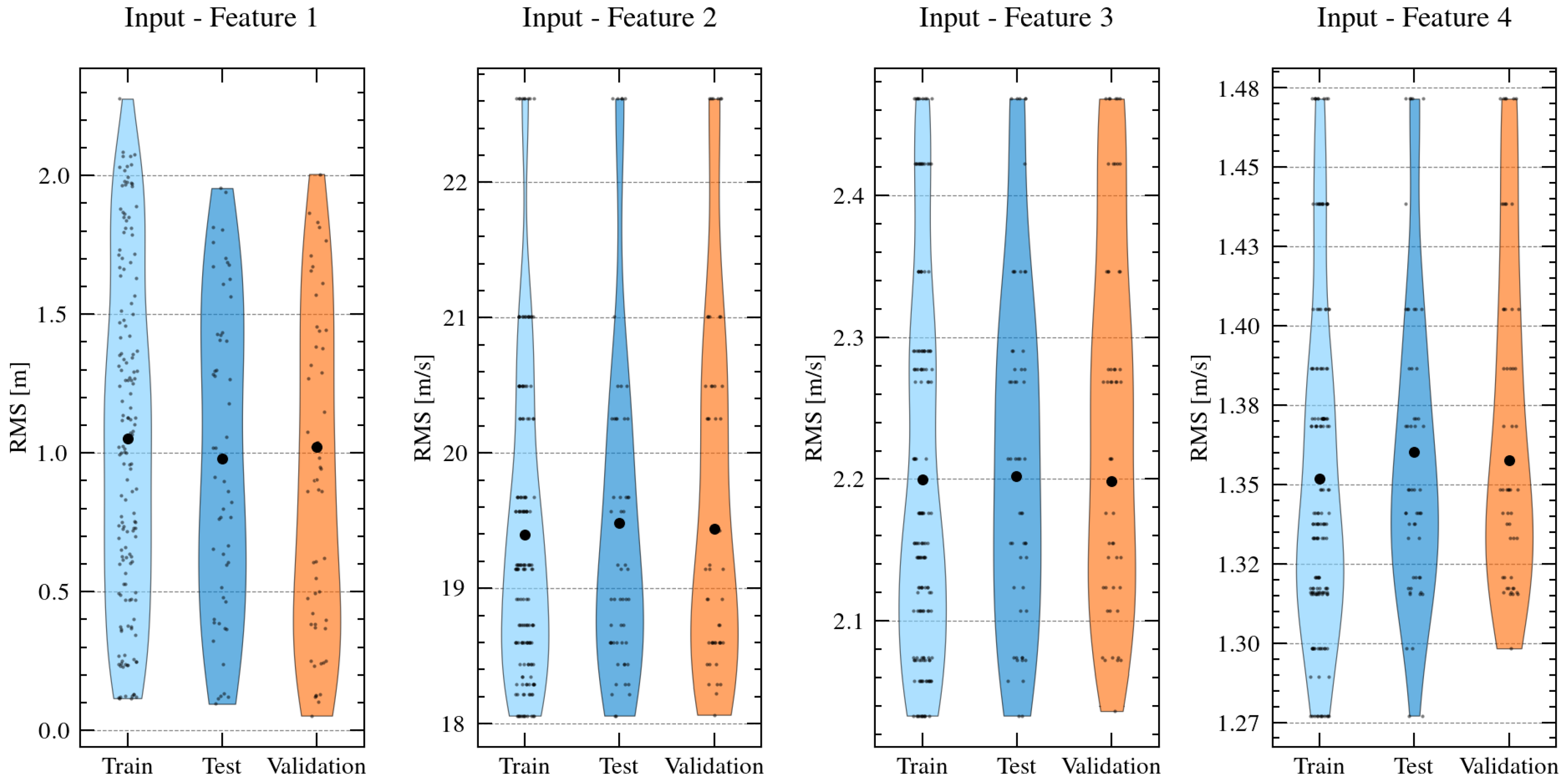
2.2. Database Generation for Training and Validation of the Neural Network Model

This FOWT was simulated under different sea states corresponding to Aberdeenshire’s coast (see Figure 2). This location is significant, as it is where the 30 MW Hywind Scotland pilot wind farm is situated [25]. Utilizing data from the wave scatter diagram, a selection of 300 irregular waves paired with turbulent wind realizations formed the Latin Hypercube sampling employed in the neural network analysis. The mean wind speed at the hub height for each wave scenario was determined using the IEC 61400 [26] power law (see Equation (1)).

$$U\left(z\right)=U_{10}{\left({\displaystyle \frac{z}{10}}\right)}^{\alpha },$$

(1)

with the recommended exponent $\alpha$ of $0.14$ [26], and z, representing the vertical distance in meters from SWL (90 $\mathrm{m}$ in this study for the hub). A range of wind speeds from 6 $\mathrm{m}/\mathrm{s}$ and 33 $\mathrm{m}/\mathrm{s}$ (above the cut-out limit for the present controller) were considered. This range includes both operational and extreme cases. One-hour simulations using OpenFAST v3.5 were conducted with different seeds (randomly uniform distributed) of the selected wind and wave spectra combination, ensuring comprehensive coverage of the FOWT’s dynamic responses under varying environmental conditions.

In the current simulations, the water depth was set at 320 m, following established literature. In addition, both waves and wind were propagating along the x-axis (180-degree heading), simplifying the complexity of actual sea states for the sake of brevity.

3. Numerical Simulations

OpenFAST is a time-domain open-source simulation tool to analyze wind turbines. In the numerical model, the spar FOWT system has been modeled using the platform properties described in Section 2.2. The platform’s hydrodynamic calculations were obtained by merging potential flow theory with Morison’s equation within OpenFAST’s HydroDyn module. The hydrodynamic coefficients obtained from frequency domain analysis are utilized in the time domain by replacing the integral over all frequency-dependent incident-wave-excitation forces [28] with a convolution integral, which in HydroDyn is implemented using Fourier transforms, as outlined by Oglive [29] and Duarte et al. [30]. In the present research, although HydroDyn (OpenFAST) primarily processes data files generated by WAMIT, ANSYS Aqwa, a commercial software for undertaking hydrodynamic and mooring analyses, was employed for the frequency domain analysis.

Then, the model was calibrated and fine-tuned using data from the available literature [31]. A similar methodology was adopted in [23]. For all DoFs, numerical decay tests were performed to calibrate the numerical model. This fine-tuning consisted of adding a quadratic viscous-drag term ($C_D$) equal to 0.6 in the horizontal direction, and an additional linear damping matrix in surge, sway, heave, and yaw, which aligns with the NREL Report [31]. Figure 3 presents an example of a time series of platform motions for both the experimental decay test and the numerical decay test of the tuned numerical model.

Furthermore, motion RAOs were obtained by running a white noise spectrum to validate the numerical model with the available numerical and experimental literature [20,32,33]. In Figure 4, a comparison of the motion RAOs obtained with the developed numerical model and the ones obtained in [20] is displayed.

In addition, the mooring system presented in [34] is modeled with MoorDyn (OpenFAST) [35], which takes into account the effect of inertia, hydrostatics, axial elasticity, structural damping, hydrodynamic added mass, and hydrodynamic drag. Bending stiffness is neglected since a chain is considered for the mooring system. The line’s contact with the seabed is modeled with a series of spring dampers.

A three-dimensional turbulent wind field was generated according to the mean wind speed at the hub height, using the power law explained previously. The TurbSim tool [36] was employed to simulate a one-hour wind time series for each case with a random realization of the Kaimal spectrum. InflowWind module processes these wind time series over the turbine and loads them in OpenFAST. Each irregular wave spectrum was generated using a random phase by HydroDyn, with seeds chosen uniformly.

Also, the aerodynamic loads on both the blades and tower were calculated within OpenFAST’s AeroDyn module. To model the operational rotor, we used dynamic Blade-Element/Momentum (DBEM) with an unsteady airfoil aerodynamic (UA) model; when the mean wind speed overpasses the cut-out limit, the rotor is set as idling, allowing it to spin freely at low speed so that the aerodynamic loads are neglected [37].

Finally, the structural dynamics of the wind turbine are computed with the ElastoDyn module, which receives the forces and the reactions, and obtains the position, velocity, and accelerations of key points of the structure. In scenarios where the turbine is not operational, the initial rotor speed is set to zero, and the blade pitch is in feathered condition. Furthermore, for these cases, the startup of the generator was disabled, and some speed-independent drag was added to the drivetrain by applying a light brake load in the ServoDyn modules [38].

4. Neural Network Model

Although several data-driven and Machine Learning (ML) models have been designed and developed for floating bodies’ motion prediction in the past, considerable challenges still remain. Regarding the Artificial Neural Network (ANN) techniques, Feedforward Neural Networks models (FNN) have been used in many time series forecastings [9], including FOWTs’ mooring lines tension logs prediction and optimization [12,16]. An FNN model is a network without recurrent links, which means the signals only pass in one direction. Data flow through the input layer, where each element calculates a weighted sum of its inputs. These computed values are then fed into the subsequent layer, and this sequence continues through each layer until the final output is produced. The output is finally optimized with the back propagation method. Nevertheless, while these basic models are effective for some tasks, they frequently struggle with high non-linearity and long-term dependencies, characteristic of complex time series data.

To address these limitations, Recurrent Neural Networks (RNNs) were developed in the 1980s [13]. Their architecture with recurrent connections enables the network to maintain a memory of previous inputs in its internal state, which is essential for capturing temporal dependencies in sequential data. However, RNNs face challenges with vanishing or exploding gradients during training. As a result, when dealing with longer sequences, RNNs may struggle to retain earlier information, complicating the learning of dependencies between distant elements within the sequence.

For this reason, in the present study, the authors employed an LSTM-based Neural Network, which mitigates the vanishing gradient problem, implemented using PyTorch. For the FOWTs’ dynamics, excited both by waves and wind, the response depends not only on the current state, but also on the previous states. This approach, distinct from traditional FNN, ensures more accurate and reliable predictions of the complex, time-dependent behavior of FOWT platforms.

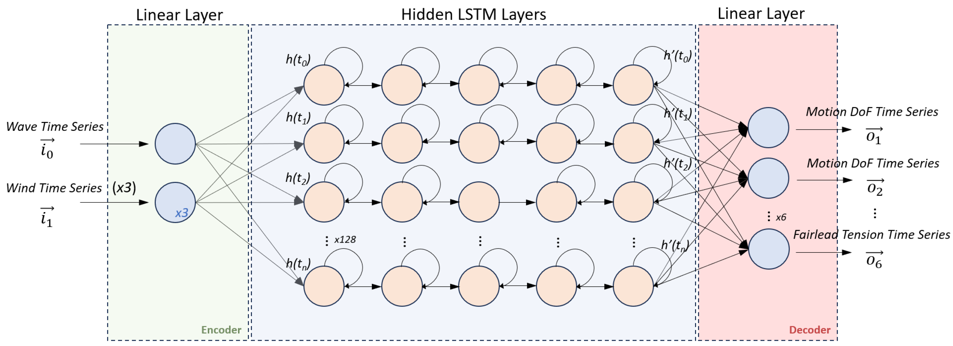
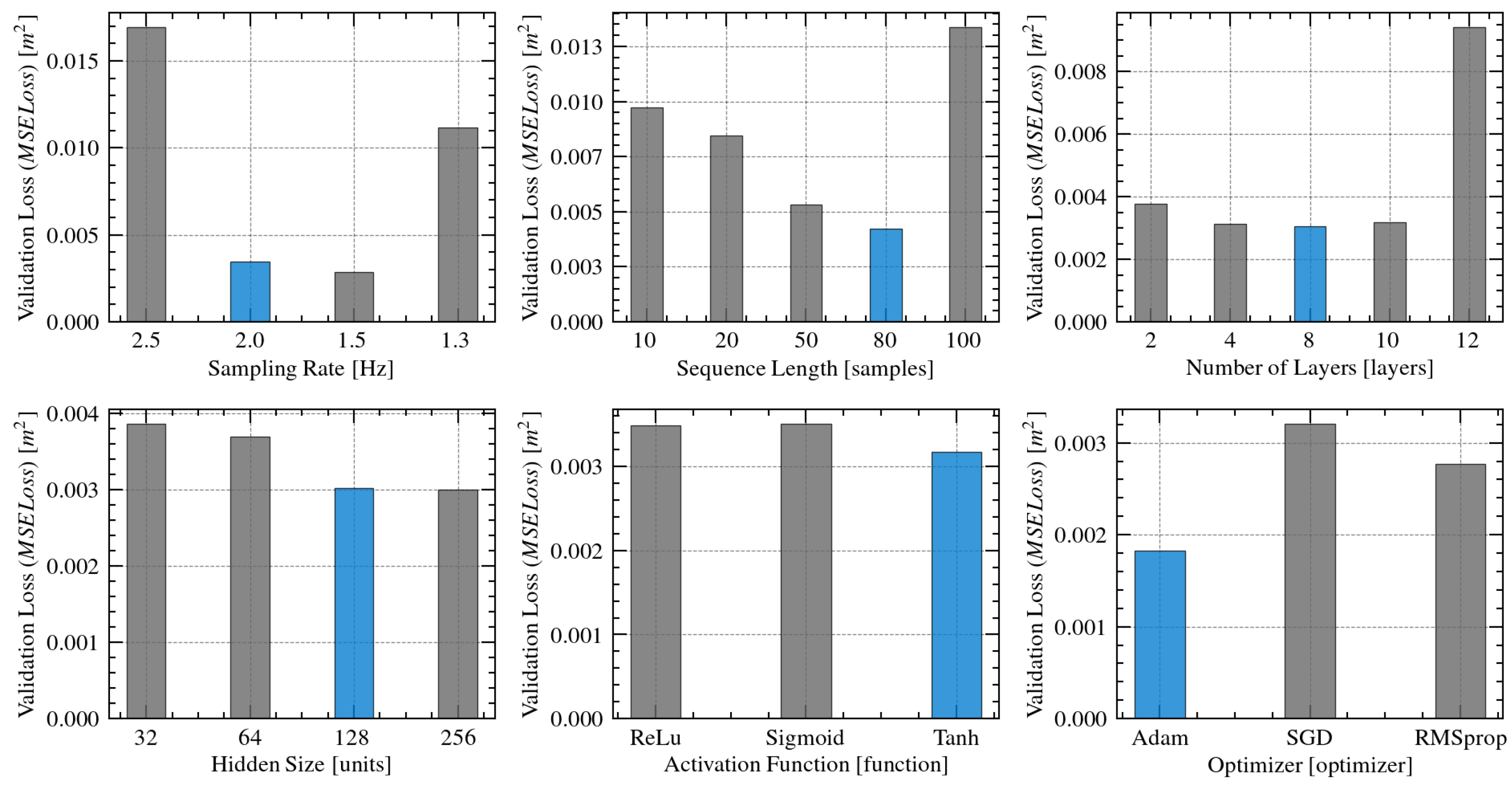
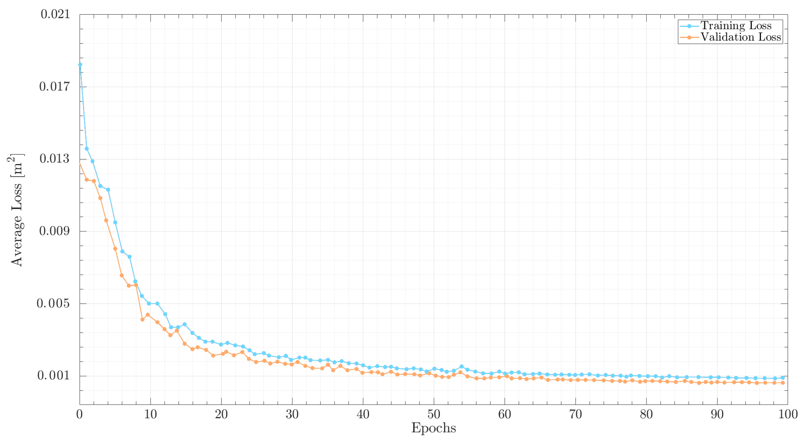
4.1. Model Architecture and Set-Up

The proposed neural network includes an input linear layer that works as an encoder and a single linear output layer that acts as a decoder, producing the time series prediction for each DoF motion. These linear layers adjust the feature space for optimal LSTM processing. The hidden layers consist of five LSTM layers, each with 128 cells, tailored to capture both complex dependencies between the input and output features and the temporal sequence information from previous time steps ($h_{t-1}$). The use of the tanh activation function ($\sigma$) across these layers enhances the model’s ability to learn intricate mappings, especially under the normalization applied here (between −1 and +1).

Figure 5 illustrates the developed neural network architecture and its data flow. The input layer is designed to collect the four excitation features as time series data. Its output is flattened into a single feature space, which feeds the subsequent five LSTM layers. Across the hidden LSTM layers, the model captures temporal dependencies sequentially in each cell. The output values from the last LSTM layer are passed to the final linear layer, which not only weights the contribution and fine-fits the LSTM-extracted data, but also reshapes it to match the desired number of output features.

Time series data of wave elevation and wind speed at each local axis of the nacelle serve as the input vectors to the LSTM model (${\eta }_{t_i}$) for a time vector t. The final predicted output (${\xi }_{t_i}$) from the developed model is each DoF motion or fairlead tension for the combination of excitations. Throughout the training, the network performs forward passes (Equation (2)) using updated weights ($W_{ih}$ and $W_{hh}$) and biases ($b_{ih}$ and $b_{hh}$) and subsequently computes gradients for backpropagation.

$${\xi }_{t_i}=\sigma ({\eta }_{t_i}{W}_{ih}^T+b_{ih}+h_{t-1}{W}_{hh}^T+b_{hh}).$$

(2)

During this training, the loss function measures the discrepancy between these predicted outputs and the reference values, quantifying the performance of the model by indicating how well it is learning and generalizing from the training data. The loss function used herein was Mean Squared Error (MSE) averaged over all datasets (see Equation (3)).

$$\mathit{L}(\xi ,\widehat{\xi })={\displaystyle \frac{1}{N}}\sum _{j=1}^N\left({\displaystyle \frac{1}{T}}\sum _{t_i=1}^T{({\xi }_{t_i}^j-{\widehat{\xi }}_{t_i}^j)}^2\right),$$

(3)

where N is the total number of cases used in each dataset, T is the total length of each time series, ${\xi }_{t_i}^j$ is the reference output, and ${\widehat{\xi }}_{t_i}^j$ is the predicted one.

In addition, optimization of the hyperparameters was carried out using the Ray Tune tool [39]. The sampling rate, sequence length, number of layers, activation function, and optimizer were some of the hyperparameters optimized to obtain the best results in the minimum training time. Figure 6 displays the validation loss over the different trials. The test colored in blue remains for the final hyperparameters employed in the NN. Despite not being the lowest loss, the improvement in loss over the computational training time of applying another hidden size or sampling rate combination is minimal.

The final model configuration employed the Adam optimizer [40] to minimize the loss during backpropagation. The chosen sequence length was 80 time steps. An initial learning rate of $0.005$ was implemented, with a decay schedule that reduced by 0.9 each epoch. The detailed hyperparameters used in the presented model are listed in

Table 2. Training matrix, neural network architecture, and hyperparameters for the developed model.

Properties	Value
Number of layers	8
Hidden size	128
Initial learning rate	0.005
Learning rate schedule	StepLR ($\gamma$ = 0.9)
Optimizer	Adam
Loss function	MSELoss
Sequence length	80
Epochs	30

.

The time series output from numerical simulations of each corresponding movement and mooring fairlead tensions are used as the training output of the network. The model’s inputs include excitation logs, i.e., sea surface elevation and turbulent wind speed vectors. Both inputs and outputs are normalized to a range between −1 and +1 based on their respective minimum and maximum values. Scaling of the features prevents vanishing or exploding gradient issues and enhances numeric stability during training.

The input data, originating from numerical simulations with an initial sampling frequency of 100 $\mathrm{Hz}$, was down-sampled to 2 $\mathrm{Hz}$ to prevent redundant information and force the model to focus on long-term dependencies. High sampling frequencies can lead to similar consecutive data samples, causing redundancy. The Nyquist theorem [41] was checked when selecting the minimum re-sampling frequency.

Finally, the dataset was randomly divided into training ($65\%$) used by the model to learn patterns; validation ($15\%$) to tune hyperparameters and prevent overfitting, but not used to update the model weights and bias; and testing ($20\%$) to assess the model’s generalization performance on unseen data and a final check. This split into subsets ensures robust model evaluation. All the datasets have been preprocessed to check if the statistical data from this split are similar. Figure 7 presents the rotated kernel densities from all the subsets from input features, i.e., wave elevation and wind speed in the X, Y, and Z directions, respectively, from left to right. It shows that similar distributions and means values are maintained across the training, validation, and testing datasets, indicating consistent statistical properties and ensuring the reliability of the model’s performance evaluations.

5. Results and Discussion

The presented ANN model was trained to predict a 30 min time series for all DoF motions and fairlead tensions, requiring 100 epochs and over 60 h of computational time in total, with the model running on a GPU with 8 GB memory. Based on [42,43], 30 min of wind and wave excitation might be considered a statistically stationary process, helping to adequately model the system’s dynamics along any longer-term patterns. Considering this, to ensure that extreme (low probability) events are well represented and captured in the model predictions, one would have to resort to either running a larger number of seeds or merging consecutive prediction periods, accounting for the variations in the statistical properties of the environmental forcing, or both. Fixing the number of seeds and looking into the time variation of the environmental forcing would deserve a separate investigation, left for future work.

This duration represents a significant improvement over similar previous studies, which only achieved accurate predictions for durations of up to 150 s [16,17,18]. Moreover, the model takes less than 5 s to infer 30 min of six DoF motions and the three fairlead tensions for each sea state, while the same case, numerically simulated within equal computation conditions, takes more than 10 min (two orders of magnitude gain).

One important aspect to assess the robustness of these type of models is to show that they do not present either overfitting or underfitting issues [44,45,46]. In the case of overfitting, the learning model can only memorize the training dataset, displaying poor results for inputs other than such a training dataset. In the case of underfitting, the learning model is too simple and cannot capture the underlying data patterns.

To verify that the model had no overfitting issues throughout the training, the losses for both training and validation datasets were monitored until they converged to a low MSE averaged value for all the predicted features. The loss curves for heave motion presented in Figure 8 exhibit similar trends for both training and validation losses, further indicating the absence of overfitting.

With regard to underfitting, from the next analysis, it will be made clear that the model is able to accurately predict the responses for the test dataset.

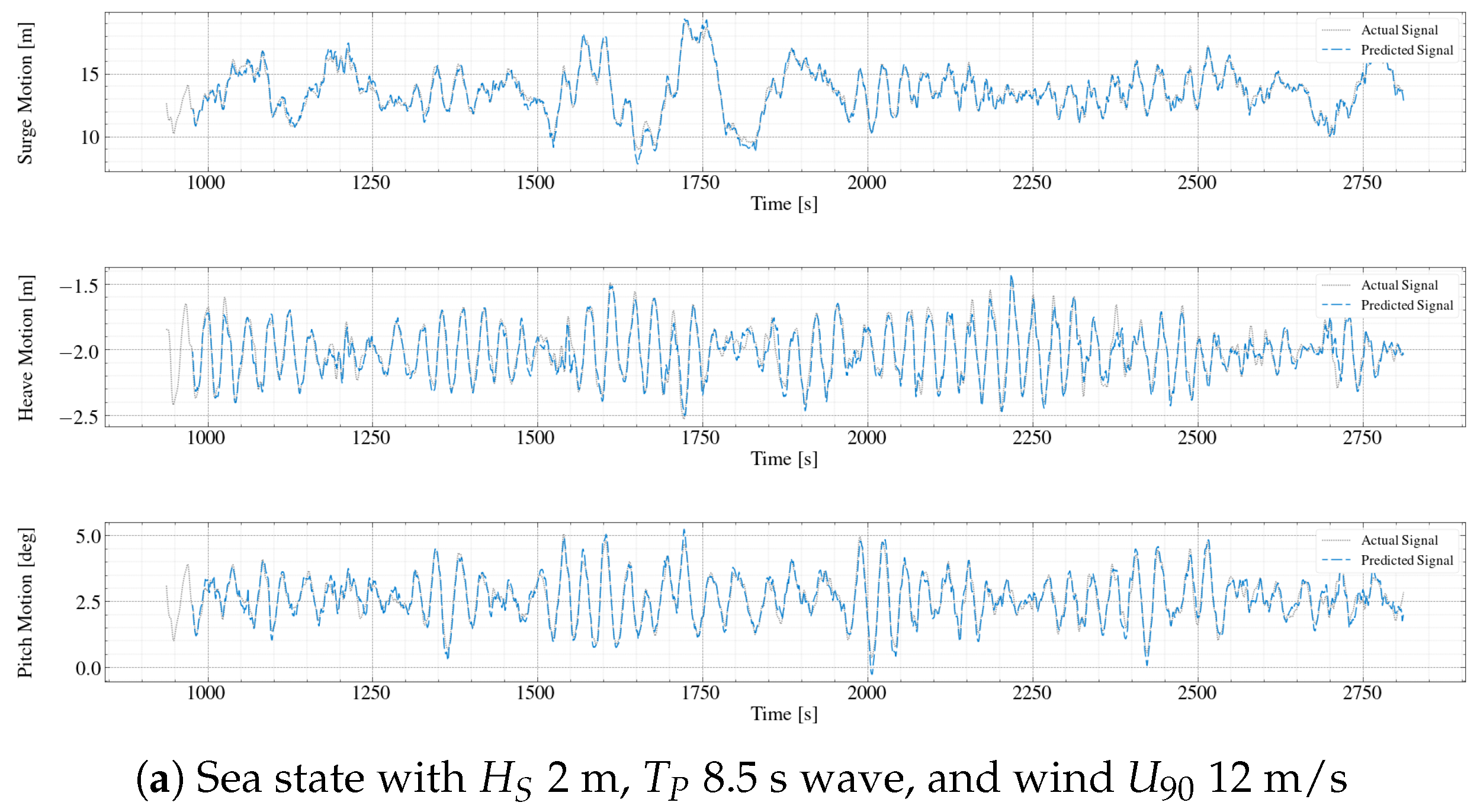
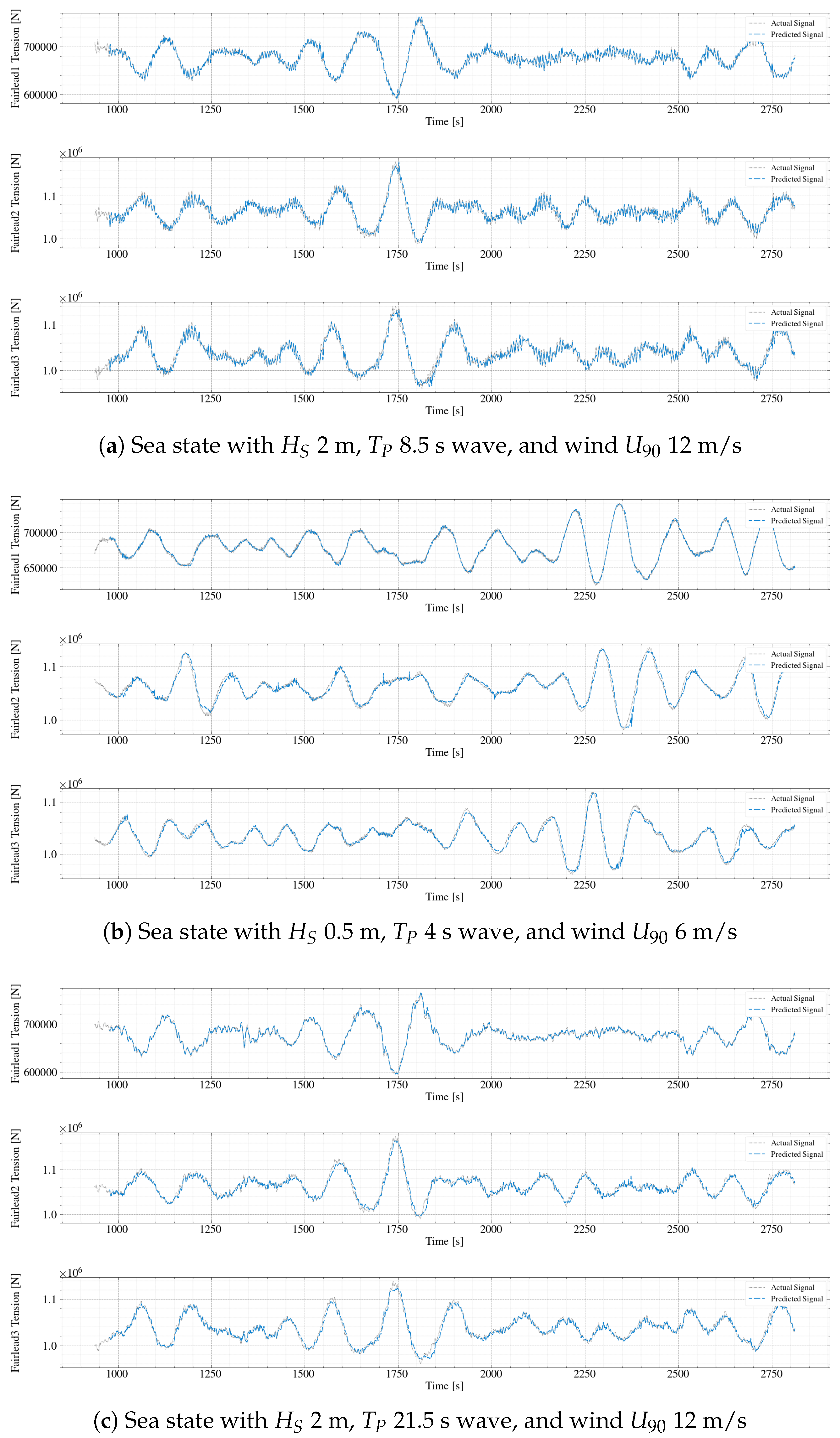
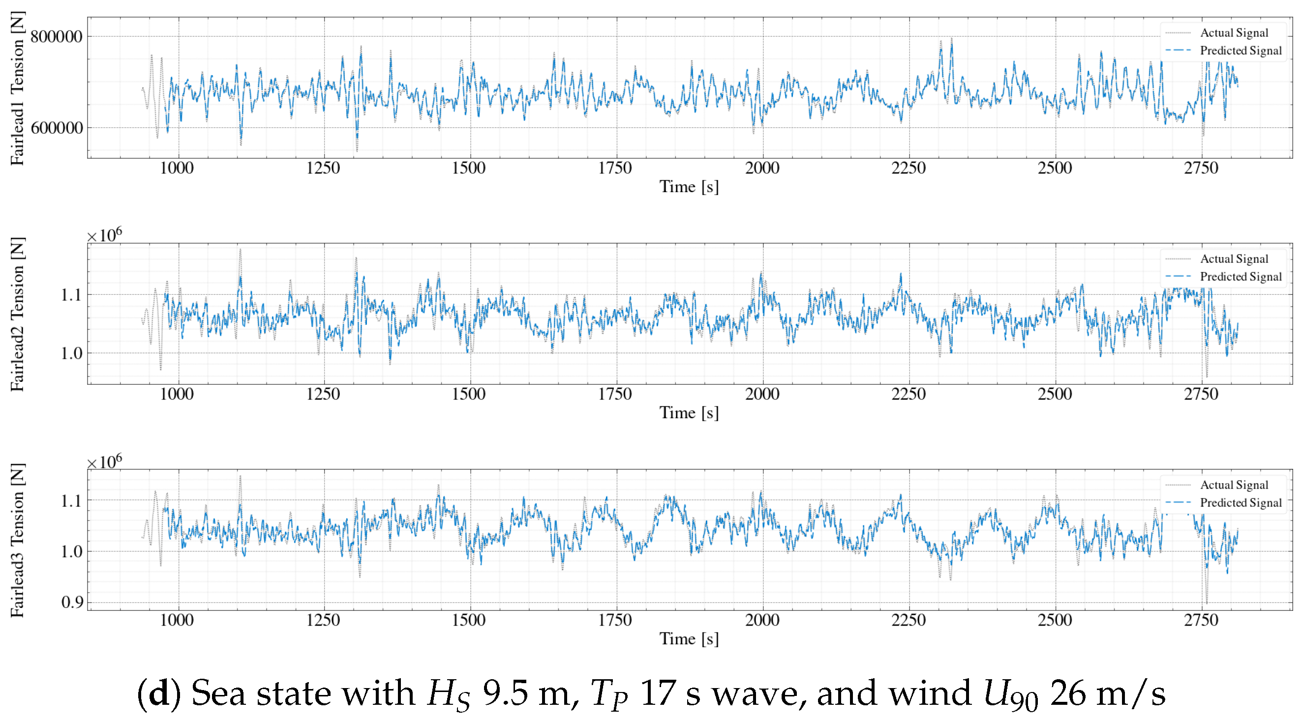
5.1. Discussion of Selected Test Cases through Analysis of Time Histories

As reported in Section 2.2, the simulated cases only include 180-degree wave directionality. For this reason, and considering the symmetry of the configuration with respect to the x-axis, the results will focus on the excited DoFs, i.e., surge, heave and pitch motions, and the three fairlead tensions. Four representative cases of the whole Convex Hull from the test dataset have been selected for the present discussion:

(a)

Irregular wave case with $H_S$ 2 m, $T_P$ 8.5 s, and turbulent wind with $U_{90}$ 12 m/s represents the operational wave with higher occurrence probability.

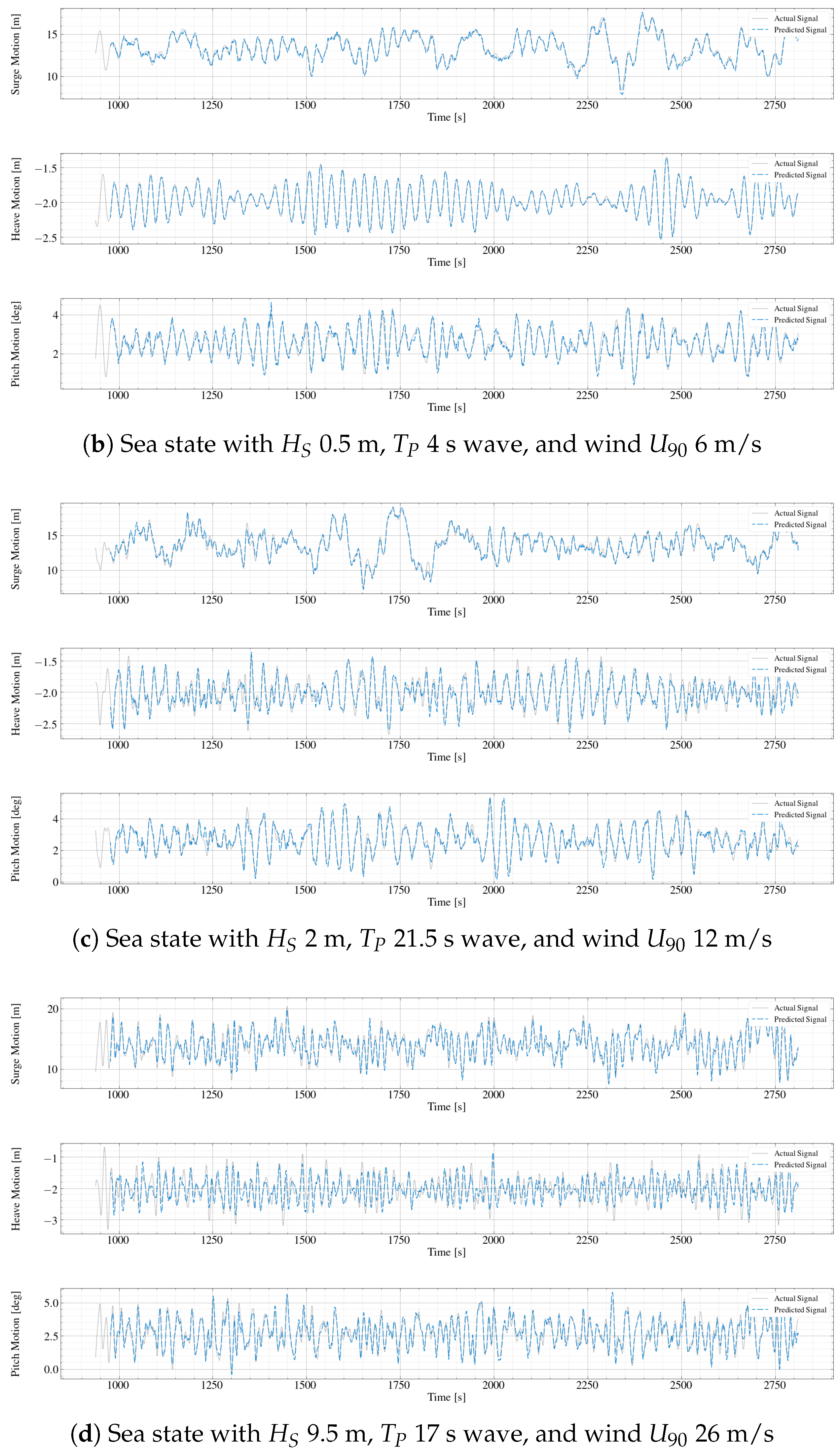
(b)

On the other hand, the case corresponding to an irregular wave with $H_S$ 3 m, $T_P$ 7 s, and a wind speed of 6 m/s for $U_{90}$ corresponds to the lowest peak period from the test dataset.

(c)

In addition, the case with $H_S$ 2 m, $T_P$ 21.5 s, and $U_{90}$ 12 m/s is within the highest peak period limits, with low observed events.

(d)

Finally, the irregular wave case with $H_S$ 9.5 m, $T_P$ 17 s, and a wind speed for $U_{90}$ of 26 m/s exemplifies the extreme sea state for the utilized scatter. In such a condition, the turbine is parked/idling.

A selection of thirty minutes of predicted outputs from these cases is presented in Figure 9 for motions and in Figure 10 for mooring loads.

The results for motions fairly match with the reference values, presented in the gray dashed line in Figure 9. Comparing the results between different DoF motions, the heave response exhibits a less accurate prediction compared to surge and pitch. This discrepancy can be attributed to the relatively smaller amplitude of the heave motion compared to the others of the DoFs, despite normalization, making it more prone to larger relative errors. Additionally, the heave motion’s principal frequency response is significantly larger than the other predicted responses, i.e., surge DoF, suggesting the need for adjustments in the sampling frequency and sequence length to improve prediction accuracy. The comparison across different sea states and wind conditions (that will be later discussed in more detail) reveals that, in general, the LSTM model demonstrates strong predictive accuracy, capturing the overall trends. In low wave and wind excitation, such as lower peak period (Figure 9a–c), all motion predictions closely follow the actual signals, showing the model’s robustness to varying periods. In extreme conditions (Figure 9d), the surge and pitch motion predictions remain reliable, albeit with major discrepancies, struggling to capture the higher rapid oscillations accurately. Heave predictions continue to show larger deviations.

Furthermore, Figure 10 displays the predicted tensions for each mooring line, with a good correlation with reference values. Fairleads 2 and 3 correspond to the up-wind ones facing the incoming waves and wind, and Fairlead 1 the down-wind one. Fairleads’ responses are largely dominated by the second-order surge mean drift response. Nevertheless, the model also captures the wave frequency, as can be seen in the operational case (Figure 10a). For the extreme case (Figure 10c), there are no noticeable differences between fairleads. In the next section, a detailed evaluation of the model’s accuracy is carried out. The analysis of the extreme events and statistic tails are beyond the scope of the present study.

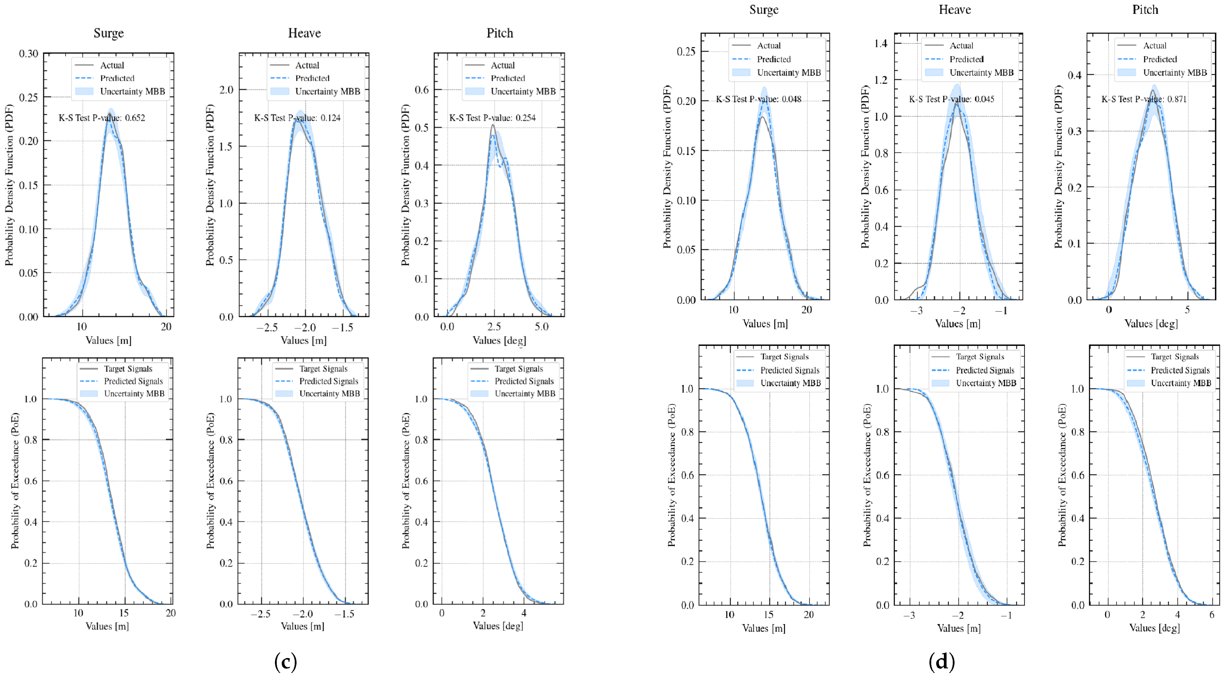
5.2. Evaluation of Selected Test Cases Using a Probabilistic Approach

Although the overall time series comparison in Figure 9 and Figure 10 suggests a strong correlation between the estimated and the reference data, further analysis has been conducted by obtaining and evaluating the heteroskedasticity ($R^2$ score) and comparing the statistics of the predicted values to those of the reference data. These metrics provide deeper insights into the model’s performance, assessing its precision in a probabilistic framework, which is useful from the industrial point of view.

Figure 11 shows the predicted and reference values for the wave cases displayed previously. Each point in the scatter represents a single time step response amplitude—motions and mooring tensions—prediction, where the input wave elevation and wind speed are identical between numerical simulation and LSTM inference. The exact 1:1 correlation would be in the straight black line. $R^2$ values are also presented for each case. In the same figure, the residual values, defined as the difference between the obtained and reference values, are presented with a grayscale legend.

It can be appreciated that the residual distribution for surge response is similar for all values and the different selected cases, with $R^2$ coefficients of around $0.97$. The pitch motion prediction displays a high degree of accuracy, with $R^2$ values above 0.9 for all the samples but lower than for surge predictions.

Regarding heave, the prediction presents a lower accuracy, except for the sea state with the smallest peak period. For this case (Figure 9b), the response is rather regular, which might help the LSTM model to predict more accurately, leading to the largest $R^2$ in Figure 11b. It is remarkable that for the largest significant wave height (cases c and d), the accuracy in the prediction for heave motions falls, in particular, for the extreme sea state, with $H_S=9.5\mathrm{m}$.

The inference of the tensions at the fairleads outcomes $R^2$ scores above $0.95$ in all the cases shown, indicating that the predictions are rather accurate.

In addition to comparing values in each time step, the Cumulative Distribution Functions (CDF) and the Probability Density Functions (PDF) of the reference and obtained values have also been compared for a comprehensive understanding of the model’s performance. These functions are crucial to enhance the understanding of the probability distribution of the predicted continuous random variables, rather than simply matching individual time steps. PDFs ensure a more robust validation of the model in capturing the underlying distribution and variability of the system, while CDFs enable an evaluation of the model’s performance in critical scenarios. In the case of the CDF, the Probability of Exceedance ($1-CDF$), PoE, is actually displayed instead, as it is of more practical value. PoEs and PDFs are presented in Figure 12 for all the cases selected for discussion. The CDFs were estimated from the PDFs using the Empirical Cumulative Distribution Function [47] of the random discrete variables, following Equation (4).

$$F\left(x\right)=P\left(X_i\le x\right)={\displaystyle \frac{1}{n}}\sum _{i=1}^n\left(X_i\le x\right),$$

(4)

where $F\left(x\right)$ is the computed CDF, n is the total number of observations, and $X_i$ are the the predicted ${\widehat{\xi }}_{t_i}$ or reference outputs ${\xi }_{t_i}$.

Upon the statistical study, the Two-Sample Kolmogorov–Smirnov Test (K–S Test) [48] was performed over all motion predictions to compare whether the two independent samples (reference and inference) were drawn from the same probabilistic distribution. In Figure 12, the K–S Test p-value results are also provided. In addition, the figure displays the 95% confidence intervals of the CDFs and PDFs, in shaded blue, computed using the Moving Block Bootstrap (MBB) method technique [49].

In the operational case, Figure 12a, the PDF of the predicted signal (blue dashed line) closely follows the reference signal’s PDF (gray solid line) for surge motion. However, for pitch and heave motions, slight deviations are visible around mean values. Focusing on the PoEs, they fairly match the reference ones, with larger deviations for heave at the upper tail. For pitch, it shows smaller predicted values in the central part of the distribution.

For cases with both lower and upper wave periods, Figure 12b,c, present, respectively, the predicted PDFs. It can be seen that they align well with the reference PDFs for surge and heave motions, with minor deviations. Some deviations are visible, especially in the central region of the distribution for pitch DoF.

The comparison of PoEs and PDFs for the extreme sea state, Figure 12d, both for surge and pitch motions, display a good correlation, except with minimum over-predictions in the peak part of the surge distribution. Nevertheless, in heave motions, the PoE shows some differences for both tails.

Focusing on the K–S Tests, the resulting p-values are above $0.05$ for most of the cases, indicating no significant difference between the predicted and reference distributions, thus confirming the reliability and accuracy of the model’s predictions even under extreme conditions.

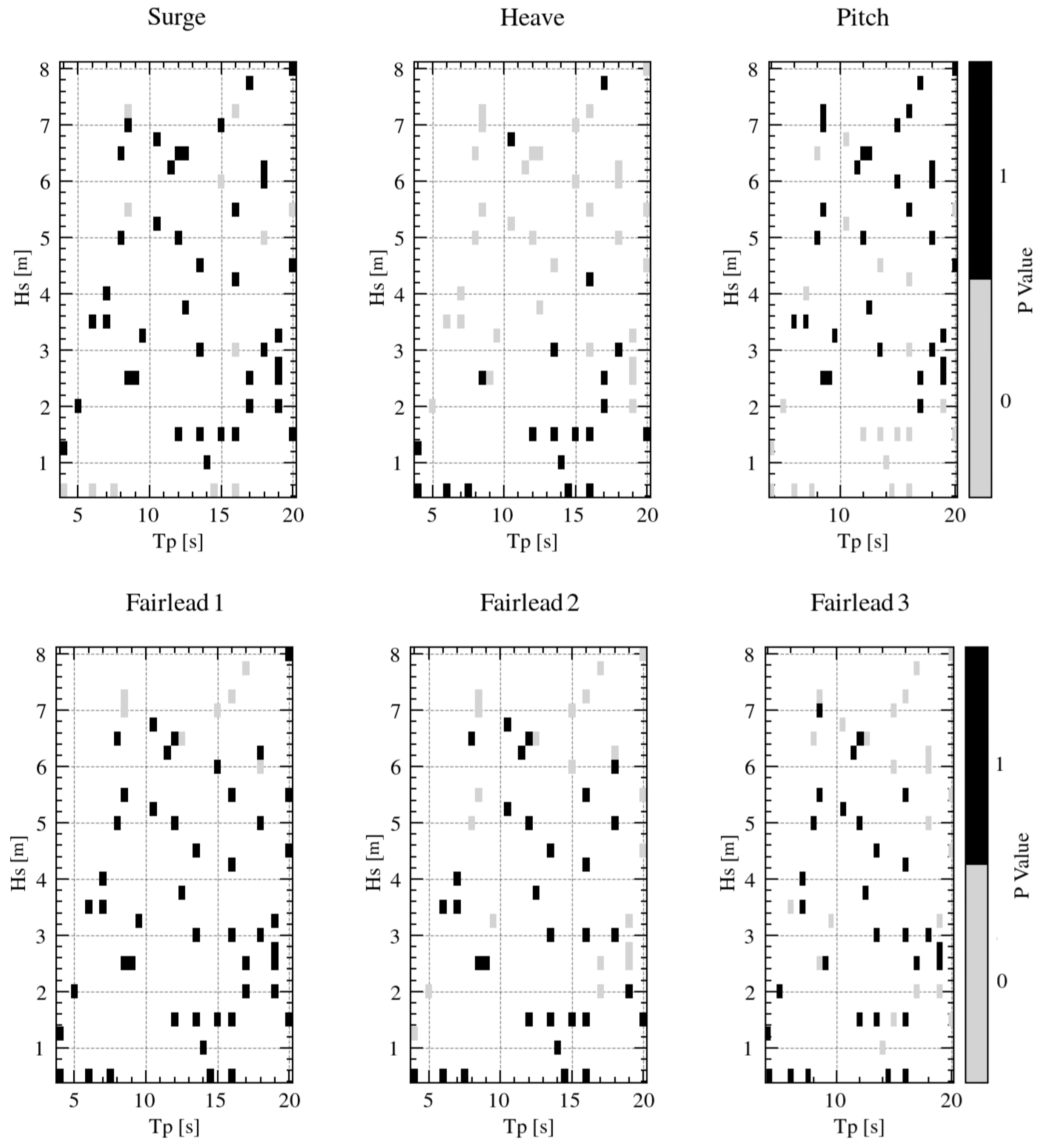
5.3. Global Evaluation of All Test Cases Using a Probabilistic Approach

Each test case can be analyzed through its $R^2$ score and the p-value from the K–S Test. To represent the accuracy of the model for all the cases in the test dataset split (see Section 4.1), heat maps along the whole Convex Hull of such a dataset are displayed in Figure 13 and Figure 14. These figures show the general behavior of the model depending on the inputs, i.e., significant wave height—or wind speed—and the peak period.

In Figure 13, the $R^2$ score for the three DoF motions and the three mooring tensions is shown. The three motions present similar distributions, with a lower correlation with the reference data in the cases with large $H_S$. This general trend was also observed for the selected cases in Section 5.1. The dependence with $T_P$ is instead negligible.

In the same Figure 13, tension predictions display high correlations for all the fairleads, with similar results for both Fairlead 2 and Fairlead 3, as expected.

The average across the whole test dataset of the $R^2$ correlation indicator has been computed for all the DoFs and fairlead tensions. Except for heave, their values are all above $0.9$ ($0.94$, $0.91$ for surge and pitch, and $0.98$, $0.94$, and $0.94$ for the three tensions). However, for the heave response, this value is $0.78$. This lower correlation is expected, considering the analysis from the selected cases in Section 5.1.

Figure 14 focuses on the p-values from the K–S Tests presented as pass (1), no-pass (0) binary heatmaps. It can be noticed that for surge and pitch motions, most of the cases pass the K–S Test of equal distribution between the reference and the predicted data. It is remarkable that for low $H_S$, there are some cases that fail the K–S Test. This could be related to the reduced response under these conditions, naturally leading to larger relative deviations.

Regarding the heave DoF, the heatmap reveals a less favorable outcome, with several cases not passing the K–S Test. Contrary to surge and pitch, the majority of cases that pass the test correspond to low $H_S$ values. Indeed, it is observed that higher $H_S$ conditions induce greater variability and non-linearity in the heave motion, making it more challenging for the model to capture the full statistical distribution of the data with accuracy. All the motions display no clear dependence on $T_P$, as for the $R^2$ analysis.

As for the fairlead tensions, one can observe that most of the cases pass the K–S Test—mainly in Fairlead 1, with $90\%$ of the cases. The majority of the failed cases are located in the range of high significant wave height, consistent with their larger dependence on the surge motion.

In brief, the presented model demonstrates high accuracy and reliability for most dynamic responses, particularly in surge and pitch motions and mooring tensions, with strong statistical consistency across various conditions.

6. Conclusions

In this paper, a comprehensive study was conducted on the prediction of the dynamics of the OC3-Hywind Floating Offshore Wind Turbine using an LSTM-based neural network model. The model was trained and validated with extensive datasets from fully coupled simulations using OpenFAST under various sea states and wind conditions, including operational and severe sea states. The following conclusions have been derived:

• The LSTM model effectively predicted time series for surge, heave, and pitch motions, as well as fairlead tensions under both operational and extreme wind and wave conditions. The model demonstrated high predictive accuracy, particularly for surge and pitch motions, with $R^2$ values generally above $0.9$.
• Statistical evaluations, including Probability Density Functions (PDFs), Cumulative Distribution Functions (CDFs), and Kolmogorov–Smirnov (K–S) Tests, confirmed the reliability of the model’s predictions. The majority of the cases passed the K–S Test, indicating that the predicted and actual distributions are very similar.
• Although the model performed well overall, the heave motion predictions were less accurate compared to surge and pitch. This discrepancy is attributed to the smaller amplitude of heave motions and their higher frequency response, indicating the need for further adjustments in sampling frequency and sequence length.
• The model significantly reduced the computational time required for predicting FOWT dynamics. While traditional numerical simulations could take more than 10 min to compute, the LSTM model inferred 30 min of time series data in less than 5 s. This reduction makes the present proposed approach relevant mainly for fatigue analysis, with aiming to discard preliminary designs.

In summary, the reliability of the developed LSTM model in predicting FOWT dynamics enables this type of model as a promising tools for its application in real-time monitoring and control strategies. This approach promises to enhance the design and operational efficiency of offshore wind energy systems.

Future research efforts will address the detailed statistical treatment of the low probable extreme values in both motions and mooring loads, focusing on particular cases such as extreme sea states and including additional quantitative metrics. Furthermore, expanding the prediction duration will allow a more in-depth analysis of the long-term behavior. Additionally, this study will extend to different types of FOWTs, and incorporate wave and wind directionality and misalignment. Further optimization of the model’s hyperparameters and architecture could also improve prediction accuracy, especially for heave motions.

References

1. IRENA. Renewable Energy Statistics 2023; Technical Report; International Renewable Energy Agency: Masdar City, United Arab Emirates, 2023. [Google Scholar]
2. DNV. Fatigue Design of Offshore Steel Structures; Technical Report; DNV: Høvik, Norway, 2021. [Google Scholar]
3. Jonkman, J.; Sclavounos, P. Development of Fully Coupled Aeroelastic and Hydrodynamic Models for Offshore Wind Turbines: Preprint. In Proceedings of the 44th AIAA Aerospace Sciences Meeting and Exhibit, Reno, NV, USA, 9–12 January 2006; Volume 16. [Google Scholar] [CrossRef]
4. Bauduin, C.; Naciri, M. A Contribution on Quasi-Static Mooring Line Damping. J. Offshore Mech. Arct. Eng.-Trans. 2000, 122, 125–133. [Google Scholar] [CrossRef]
5. Senra, S.; Corrêa, F.; Jacob, B.; Mourelle, M.; Masetti, I. Towards the Integration of Analysis and Design of Mooring Systems and Risers: Part I—Studies on a Semisubmersible Platform. In Proceedings of the OMAE 2022, Oslo, Norway, 23–28 June 2002. [Google Scholar] [CrossRef]
6. Low, Y.; Langley, R. A hybrid time/frequency domain approach for efficient coupled analysis of vessel/mooring/riser dynamics. Ocean Eng. 2008, 35, 433–446. [Google Scholar] [CrossRef]
7. Mushtaq, M.; Akram, U.; Aamir, M.; Ali, H.; Zulqarnain, M. Neural Network Techniques for Time Series Prediction: A Review. JOIV Int. J. Inform. Vis. 2019, 3, 314–320. [Google Scholar] [CrossRef]
8. Wu, H.; Luo, Q.; Abdel-Basset, M. Training Feedforward Neural Networks Using Symbiotic Organisms Search Algorithm. Comput. Intell. Neurosci. 2016, 2016, 1–14. [Google Scholar] [CrossRef]
9. Abdulkarim, S.; Garko, A. Evaluating feedforward and elman recurrent neural network in time series forecasting. Indian J. Pure Appl. Math. 2015, 1, 145–151. [Google Scholar]
10. Serrano-Cinca, C. Feedforward Neural Networks in the Classification of Financial Information. Eur. J. Financ. 1998, 3, 183–202. [Google Scholar] [CrossRef]
11. Chen, M.; Jiang, J.; Zhang, W.; Li, C.B.; Zhou, H.; Jiang, Y.; Sun, X. Study on Mooring Design of 15 MW Floating Wind Turbines in South China Sea. J. Mar. Sci. Eng. 2023, 12, 33. [Google Scholar] [CrossRef]
12. Jiang, Y.; Duan, Y.; Li, J.; Chen, M.; Zhang, X. Optimization of mooring systems for a 10MW semisubmersible offshore wind turbines based on neural network. Ocean Eng. 2024, 296, 117020. [Google Scholar] [CrossRef]
13. Rumelhart, D.E.; Hinton, G.E.; Williams, R.J. Learning Internal Representations by Error Propagation. In Parallel Distributed Processing: Explorations in the Microstructure of Cognition, Volume 1: Foundations; Rumelhart, D.E., Mcclelland, J.L., Eds.; MIT Press: Cambridge, MA, USA, 1986; pp. 318–362. [Google Scholar]
14. Hochreiter, S.; Schmidhuber, J. Long Short-term Memory. Neural Comput. 1997, 9, 1735–1780. [Google Scholar] [CrossRef]
15. Van Houdt, G.; Mosquera, C.; Nápoles, G. A Review on the Long Short-Term Memory Model. Artif. Intell. Rev. 2020, 53, 5929–5955. [Google Scholar] [CrossRef]
16. Bjørni, F.; Lien, S.; Midtgarden, T.; Kulia, G.; Verma, A.; Jiang, Z. Prediction of dynamic mooring responses of a floating wind turbine using an artificial neural network. IOP Conf. Ser. Mater. Sci. Eng. 2021, 1201, 012023. [Google Scholar] [CrossRef]
17. Silva, K.M.; Maki, K.J. Data-Driven system identification of 6-DoF ship motion in waves with neural networks. Appl. Ocean Res. 2022, 125, 103222. [Google Scholar] [CrossRef]
18. Lee, J.H.; Lee, J.; Kim, Y.; Ahn, Y. Prediction of wave-induced ship motions based on integrated neural network system and spatiotemporal wave-field data. Phys. Fluids 2023, 35, 097127. [Google Scholar] [CrossRef]
19. Park, H.J.; Kim, J.S.; Nam, B.; Kim, J.S. ANN-based prediction models for green water events around a FPSO in irregular waves. Ocean Eng. 2024, 291, 116408. [Google Scholar] [CrossRef]
20. Jonkman, J.; Musial, W. Offshore Code Comparison Collaboration (OC3) for IEA Wind Task 23 Offshore Wind Technology and Deployment; Technical Report; NREL: Golden, CO, USA, 2010. [Google Scholar]
21. Xu, X.; Day, S. Experimental investigation on dynamic responses of a spar-type offshore floating wind turbine and its mooring system behaviour. Ocean Eng. 2021, 236, 109488. [Google Scholar] [CrossRef]
22. Yang, J.; He, Y.P.; Zhao, Y.S.; Shao, Y.L.; Han, Z.L. Experimental and numerical studies on the low-frequency responses of a spar-type floating offshore wind turbine. Ocean Eng. 2021, 222, 108571. [Google Scholar] [CrossRef]
23. Browning, J.; Jonkman, J.; Robertson, A.; Goupee, A. Calibration and validation of a spar-type floating offshore wind turbine model using the FAST dynamic simulation tool. J. Phys. Conf. Ser. 2014, 555, 012015. [Google Scholar] [CrossRef]
24. JM, J.; Butterfield, S.; Musial, W.; Scott, G. Definition of a 5MW Reference Wind Turbine for Offshore System Development; National Renewable Energy Laboratory (NREL): Golden, CO, USA, 2009. [Google Scholar] [CrossRef]
25. Burns, R.D.; Martin, S.B.; Wood, M.A.; Wilson, C.C.; Lumsden, E.; Pace, F. Hywind Scotland Floating Offshore Wind Farm; Technical Report; JASCO Applied Sciences: Silver Spring, MD, USA, 2022. [Google Scholar]
26. IEC 61400-3-2; Wind Energy Generation Systems-Part 3-2: Design Requirements for Floating Offshore Wind Turbines. Technical Report; International Electrotechnical Commission (IEC): Geneva, Switzerland, 2023.
27. Reistad, M.; Breivik, O.; Haakenstad, H.; Aarnes, O.; Furevik, B.; Bidlot, J. A high-resolution hindcast of wind and waves for The North Sea, The Norwegian Sea and The Barents Sea. J. Geophys. Res. 2011, 116. [Google Scholar] [CrossRef]
28. Cummins, W.; Taylor, D.W. The Impulse Response Function and Ship Motions; Report (David W. Taylor Model Basin); Department of the Navy, David Taylor Model Basin: Bethesda, MD, USA, 1962. [Google Scholar]
29. Oglive, T. Recent progress toward the understanding and prediction of ship motions. In Proceedings of the 5th Symposium on Navan Hydrodynamics, Bergen, Norway, 10–12 September 1964; Volume 1, p. 80. [Google Scholar]
30. Duarte, T.; Alves, M.; Jonkman, J.; Sarmento, A. State-Space Realization of the Wave-Radiation Force Within FAST. In Proceedings of the International Conference on Offshore Mechanics and Arctic Engineering, Nantes, France, 8–13 June 2013. OMAE2013-10375. [Google Scholar] [CrossRef]
31. Jonkman, J.M. Dynamics Modeling and Loads Analysis of an Offshore Floating Wind Turbine; NREL/TP-500-41958; National Renewable Energy Laboratory: Golden, CO, USA, 2007. [Google Scholar] [CrossRef]
32. Tomasicchio, G.R.; D’Alessandro, F.; Avossa, A.M.; Riefolo, L.; Musci, E.; Ricciardelli, F.; Vicinanza, D. Experimental modelling of the dynamic behaviour of a spar buoy wind turbine. Renew. Energy 2018, 127, 412–432. [Google Scholar] [CrossRef]
33. Lopez-Olocco, T.; Liang, G.; Medina-Manuel, A.; Ynocente, L.S.; Jiang, Z.; Souto-Iglesias, A. Experimental comparison of a dual-spar floating wind farm with shared mooring against a single floating wind turbine under wave conditions. Eng. Struct. 2023, 292, 116475. [Google Scholar] [CrossRef]
34. Jonkman, J. Definition of the Floating System for Phase IV of OC3; Number NREL/TP-500-47535; National Renewable Energy Laboratory: Golden, CO, USA, 2010. [Google Scholar]
35. Hall, M.; Goupee, A. Validation of a lumped-mass mooring line model with DeepCwind semisubmersible model test data. Ocean Eng. 2015, 104, 590–603. [Google Scholar] [CrossRef]
36. Jonkman, J.M. TurbSim User’s Guide v2.00.00. Revised June 1, 2016 (Draft Version); Technical Report; National Renewable Energy Lab (NREL): Golden, CO, USA, 2016. [Google Scholar]
37. Jonkman, J.M.; Buhl, M.L., Jr. Fast User’s Guide-Updated August 2005; Technical Report; National Renewable Energy Lab (NREL): Golden, CO, USA, 2005. [Google Scholar]
38. National Renewable Energy Lab. OpenFAST Documentation-Release v2.3.0; Technical Report; National Renewable Energy Lab (NREL): Golden, CO, USA, 2020. [Google Scholar]
39. Liaw, R.; Liang, E.; Nishihara, R. Tune: A Research Platform for Distributed Model Selection and Training. arXiv 2018, arXiv:1807.05118. [Google Scholar]
40. Kingma, D.P.; Ba, J. Adam: A Method for Stochastic Optimization. arXiv 2017, arXiv:1412.6980. [Google Scholar]
41. Shannon, C. Communication in the Presence of Noise. Proc. IRE 1949, 37, 10–21. [Google Scholar] [CrossRef]
42. Goda, Y. Random Seas and Design of Maritime Structures; University of Tokyo Press: Tokyo, Japan, 1985. [Google Scholar]
43. ROM 1.0-09; Recommendations for the Project Design and Construction of Breakwaters (Part I: Calculation and Project Factors. Climate Agents). Technical Report; Puertos del Estado (PdE): Madrid, Spain, 2009.
44. Nowlan, S.J.; Hinton, G.E. Simplifying Neural Networks by Soft Weight-Sharing. Neural Comput. 1992, 4, 473–493. [Google Scholar] [CrossRef]
45. Dietterich, T. Overfitting and undercomputing in machine learning. ACM Comput. Surv. 1995, 27, 326–327. [Google Scholar] [CrossRef]
46. Bejani, M.M.; Ghatee, M. A systematic review on overfitting control in shallow and deep neural networks. Artif. Intell. Rev. 2021, 54, 6391–6438. [Google Scholar] [CrossRef]
47. Serfling, R. Approximation Theorems of Mathematical Statistics; John Wiley & Sons: New York, NY, USA, 1980. [Google Scholar] [CrossRef]
48. Smirnov, N.V. Estimate of deviation between empirical distribution functions in two independent samples. Bull. Mosc. Univ. 1939, 2, 3–16. [Google Scholar]
49. Fitzenberger, B. The moving blocks bootstrap and robust inference for linear least squares and quantile regressions. J. Econ. 1998, 82, 235–287. [Google Scholar] [CrossRef]
Figure 1. Sketch of the NREL 5 MW wind turbine on the OC3-Hywind spar. Source: Jonkman and Musial [20].
Jmse 12 01464 g001
Figure 2. Database scatter based on WAM10 wave model for the grid at 56.45° N, 02.29° W [27]. The dataset provides data from 1 September 1957 to 31 December 2010, interpolated to 3 h intervals. This point corresponds to the closest grid point to the Inch Cape site.
Jmse 12 01464 g002
Figure 3. Surge platform motions in the numerical and NREL Report [20] decay tests.
Jmse 12 01464 g003
Figure 4. OC3-Hywind RAOs’ obtained with the present model simulation framework and validated with NREL Report [20].
Jmse 12 01464 g004
Figure 5. Diagram of the LSTM neural network architecture. Blue color in cells stands for linear (fully connected) neurons and orange for LSTM neurons.
Jmse 12 01464 g005
Figure 6. Validation loss after 20 epochs from the optimization of the hyperparameters using Ray Tune. Blue bars remain for the final hyperparameters employed in the NN model.
Jmse 12 01464 g006
Figure 7. Violin plots of the Root Mean Square of the input features from the training, validation, and tests subsets.
Jmse 12 01464 g007
Figure 8. Loss convergence curves for training and validation over the epochs while training heave motion.
Jmse 12 01464 g008
Figure 9. Predicted vs. actual motions of the OC3 FOWT under various sea states and wind conditions. Each subplot compares the predicted signal (blue) with the actual signal (gray) for surge, heave, and pitch motions.
Jmse 12 01464 g009aJmse 12 01464 g009b
Figure 10. Predicted vs. actual fairlead tensions of the OC3 FOWT under various sea states and wind conditions. Each subplot compares the predicted signal (blue) with the actual signal (gray) for Fairlead 1, Fairlead 2, and Fairlead 3 tensions.
Jmse 12 01464 g010aJmse 12 01464 g010b
Figure 11. R 2 scores and residual values for specified wave trains tested. (a) Sea state with H S 2 m, T P 8.5 s wave, and wind U 90 12 m/s. (b) Sea state with H S 0.5 m, T P 4 s wave, and wind U 90 6 m/s. (c) Sea state with H S 2 m, T P 21.5 s wave, and wind U 90 12 m/s. (d) Sea state with H S 9.5 m, T P 17 s wave, and wind U 90 26 m/s.
Jmse 12 01464 g011
Figure 12. Statistics (PDFs and CDFs) of the selected cases. (a) Sea state with H S 2 m, T P 8.5 s wave, and wind U 90 12 m/s. (b) Sea state with H S 0.5 m, T P 4 s wave, and wind U 90 6 m/s. (c) Sea state with H S 2 m, T P 21.5 s wave, and wind U 90 12 m/s. (d) Sea state with H S 9.5 m, T P 17 s wave, and wind U 90 26 m/s.
Jmse 12 01464 g012aJmse 12 01464 g012b
Figure 13. Distribution of the R 2 for all the test cases.
Jmse 12 01464 g013
Figure 14. p-value from the K–S Test for all the test cases. Significance level of the tests chosen was α = 0.05 .
Jmse 12 01464 g014