Abstract
A comprehensive study was conducted at a wave energy device test site located off the northeastern coast of Taiwan to assess the influence of oceanic currents on experimental equipment. A bottom-mounted 600 kHz acoustic Doppler current profiler, equipped with integrated temperature and pressure sensors, was deployed at a depth of approximately 31 m. This study, spanning from 6 June 2023 to 11 May 2024, recorded ocean current profiles by assembling data from 50 pings every 10 min, with a resolution of one meter per depth layer. The findings reveal that variations in water levels were predominantly influenced by the M2 tidal constituent, followed by the O1, K1, and S2 tides. Notably, seawater temperature fluctuations at the seabed were modulated by tides, especially the M2 tide. A significant drop in seawater temperature was also observed as the typhoon passed through the south of Taiwan. In terms of sea surface currents, the measured maximum current speed was 71.89 cm s−1, but the average current speed was only 15.47 cm s−1. Tidal currents indicated that the M4 and M2 tides were the most significant, with semimajor axes and inclination angles of 8.48 cm s−1 and 102.60°, and 7.00 cm s−1 and 97.76°, respectively. Seasonally, barotropic tidal currents were the strongest in winter. Additionally, internal tides were identified, with the first baroclinic mode being dominant. The zero-crossing depths varied between 14 and 18 m. During the summer, the M2 baroclinic tidal current displayed characteristics of the second baroclinic mode, with zero-crossing depths at approximately 7 m and 22 m. This node aligns with results from the empirical orthogonal function analysis and correlates with the depths’ significant shifts in seawater temperature as measured by a conductivity, temperature, and depth instrument. Despite the velocities of internal tides not being strong, the directional variance between surface and bottom flows presents critical considerations for the deployment and operation of moored wave energy devices.
1. Introduction
The urgency to mitigate the effects of global warming has led to the rapid adoption of renewable energy sources, a key shift supported by a large body of recent research [,,,]. Among these renewable energy sources, ocean energy stands out for its huge and underexploited potential []. Particularly, ocean wave energy, known for its higher energy density relative to other forms of renewable energy, is rapidly becoming a focus of development []. To improve the efficiency of wave power generation, various innovative wave power generation devices have been designed []. Before widespread deployment, these devices must undergo rigorous testing in real marine environments to evaluate their performance under real operating conditions.
The National Taiwan Ocean University (NTOU), located at the northeastern tip of Taiwan and adjacent to the East China Sea, provides an ideal setting for such an assessment. NTOU’s proximity to the sea provides not only academic insights but also logistical support to facilitate extensive field testing. The key instrument in these efforts is a bottom-mounted acoustic Doppler current profiler (ADCP) strategically placed at coordinates 25.15578° N, 121.78147° E, at a depth of approximately 31 m (Figure 1). The ADCP used in this study is the Teledyne RD Instruments (RDI) WorkHorse Sentinel 600 kHz, made by TRDI at San Diego, CA, USA, which helps profile coastal currents and is critical for assessing dynamic loads on offshore structures. Understanding these ocean currents is critical because they influence sediment transport, ship navigation, and are affected by factors such as tides, waves, wind, and river plumes []. Their effects vary from hour to season and therefore require detailed and continuous monitoring [].
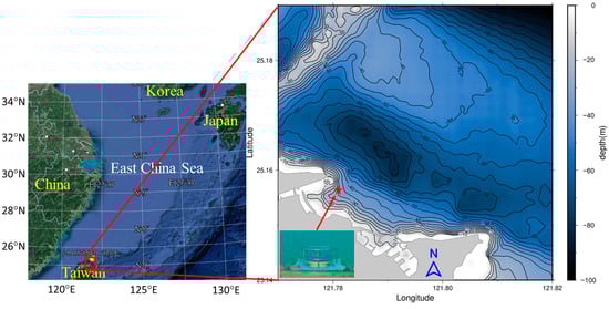
Figure 1.
The location of the ADCP deployed.
Tides are particularly significant in shaping coastal currents. The interaction between tidal movements and coastal contours not only dictates the flow patterns but also plays a pivotal role in ocean circulation and marine ecosystems [,,]. Moreover, the distinction between barotropic and baroclinic components within the tidal currents adds a layer of complexity. Internal tides, also known as baroclinic tides, occur when stratified water columns move vertically in response to seabed topography and behaves similarly to internal waves at tidal frequencies [,,,,,,]. The study of these phenomena is essential for a holistic understanding of ocean dynamics and their implications for marine energy exploitation.
By deploying advanced measurement techniques such as ADCP and leveraging the academic capabilities of institutions such as NTOU, researchers can collect critical data to optimize the design and layout of wave energy converters, thereby increasing the efficiency and feasibility of harnessing ocean wave energy.
2. Materials and Methods
A bottom-mounted ADCP was deployed at a water depth of approximately 31 m off the northeastern coast of Taiwan, aimed at measuring nearshore ocean current profiles in an area designated for ocean wave energy device testing. The ADCP collected ocean current profiles from 6 June 2023 to 11 May 2024 by ensembling 50 pings every 10 min to produce current profiles at one-meter depth intervals. Data within three meters of the sea surface were discarded due to interference from sound wave reflections. The placement of the ADCP’s frame also restricted data collection to a minimum of three meters above the seabed, effectively covering a depth range from 3 to 28 m. Equipped with both pressure and temperature sensors, this ADCP also simultaneously recorded sea surface level and seawater temperature at the depth of the ADCP to provide a comprehensive dataset. There are two thermometers attached to the ADCP. One is the ambient temperature sensor, which is mounted on the receiver board embedded in the transducer head and is used for water temperature reading. The other is the attitude temperature sensor, which is mounted on the board under the compass. In this study, the water temperature was reading from the ambient temperature sensor file. The pressure sensor recorded the pressure at the ADCP-mounted depth, which is the sum of water and atmospheric pressures. Sea level variations derived from the ADCP pressure sensor were adjusted for air pressure.
Nearshore currents are significantly affected by tides, so the harmonic analysis was used to obtain the primary tidal constituents of ocean currents and sea levels. The T_tide package [], a widely utilized tool for tidal harmonic analysis, was integral to this study. For tidal currents, each tidal constituent can be represented by a combination of barotropic and baroclinic tides. Baroclinic tides can be represented as a superposition of discrete baroclinic modes that depend on the buoyancy frequency []. However, due to the absence of continuous hydrological data across the measurement period and only a single conductivity, temperature, and depth (CTD) measurement available at the time of ADCP recovery on 11 May 2024, it was difficult to calculate the buoyancy frequency for the entire measurement period. Consequently, the empirical orthogonal function (EOF) method was adopted to decompose the vertical structure of baroclinic tidal currents, as this technique is renowned for its effectiveness in elucidating the vertical structure of baroclinic velocities [,,,].
Barotropic tidal currents are primarily generated by astronomical forcing and are invariant with depth. They were approximated by averaging the currents across all measured depths [,,]. Baroclinic tidal currents were then derived by subtracting these averaged barotropic currents from the original tidal currents. The EOF estimates of baroclinic modes were compared against those obtained through depth-averaging, which typically provides a reliable approximation of barotropic tidal currents except near surface and seabed boundaries. Despite the general utility of depth-averaging, the EOF method was noted to retain the frictional boundary layer effects within most barotropic tidal current modes [,,].
Furthermore, the EOF analysis of vectored currents was conducted using real functions rather than complex notation, despite the slower convergence rate associated with real functions. This approach was chosen because real function analysis offers more tangible insights into the physical processes involved []. The EOF decomposition can be expressed as [,]
where is the current data at depth z that changes with time t, is the time function, which is the principal component, and is the spatial function, that is, eigenvectors. In this study, the singular value decomposition technique was applied to obtain EOFs, eigenvalues, and PCs directly from the data matrix.
3. Results and Discussion
3.1. Sea Level
The bottom-mounted ADCP has a pressure sensor that measures sea level variations. Figure 2 shows the time series of sea level during the measurement period. It shows that sea level variations are mainly related to tide periods, including diurnal tide, semidiurnal tide, and the spring–neap tide. However, there seemed to be a large variation around 3 August 2023 that returned to normal after 5 August 2023. This is possibly caused by Typhoon Khanun (2023) passing by the water northeast of Taiwan on 3 August. Information about typhoons affecting Taiwan during the measurement period is introduced in the next section.
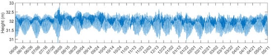
Figure 2.
Time series of sea level.
Figure 3 presents the power spectra of sea level variations, identifying several prominent tidal periods. These include diurnal tides (O1, K1, Q1), semidiurnal tides (M2, S2, N2), and overtides, such as the 1/3 period of diurnal tides (M3, MK3, MO3), the 1/4 period of diurnal tides (M4, MS4, MN4), and the 1/6 period of diurnal tides (M6, 2MS6). Overtides are astronomical constituents generated by the nonlinear effects in shallow coastal waters. Harmonic analysis was conducted to determine the amplitudes and phases of the tidal constituents showcased in Figure 3, with the results tabulated in Table 1. The analysis reveals that the M2 tide exhibits the highest amplitude, followed by the K1, O1, and S2 tides. The amplitude ordering obtained by harmonic analysis is consistent with the power ordering obtained by power spectrum.
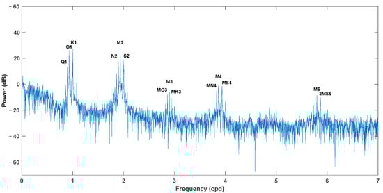
Figure 3.
Power spectrum of sea level.

Table 1.
Period, amplitude, and phase of major tidal constituents for sea level from harmonic analysis.
3.2. Seawater Temperature
The ADCP utilized in this study was equipped with a temperature sensor, which recorded the seawater temperature at the sensor’s depth. As shown in Figure 4, the time series of seawater temperature indicates noticeable reductions during specific periods. Throughout the measurement period, five typhoons approached Taiwan, with their warning times issued by Taiwan’s Central Weather Administration, detailed in Table 2, and their paths depicted in Figure 5. Notably, all typhoons except for Typhoon Khanun (2023), which traversed north of Taiwan, passed south of the island. The temporal proximity of these typhoons to marked decreases in seawater temperature suggests a direct correlation between typhoon activity and temperature drops in the sea. The periods of typhoon warnings are also marked in Figure 4, illustrating that each of the five typhoons precipitated a drop in seawater temperatures. Specifically, Typhoons Doksuri (2023) and Haikui (2023), which passed south of Taiwan, induced a cooling of approximately 10 °C, whereas Typhoon Khanun (2023), moving through northern Taiwan, resulted in a lesser cooling of about 5 °C.
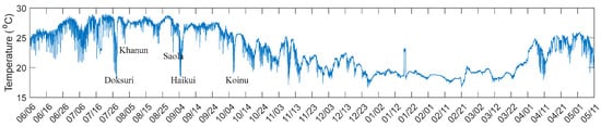
Figure 4.
Time series of seawater temperature at the depth of the sensor.
Table 2.
Warning period of typhoon approaching Taiwan issued by Central Weather Administration of Taiwan during the measuring period.
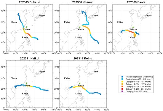
Figure 5.
The path of the typhoon approaching Taiwan during the measuring period. The asterisks in the figure are the ADCP deployment locations. Typhoon path data are taken from the National Centers for Environmental Information, National Oceanic and Atmospheric Administration at https://www.ncei.noaa.gov/products/international-best-track-archive (accessed on 1 September 2024).
Given that the ADCP was deployed north of Taiwan, the observed temperature reductions were more pronounced when typhoons passed crossing the south. This discrepancy is likely attributable to wind–tide resonance []. When typhoons pass south of Taiwan, their southeasterly wind direction aligns with the tidal currents flowing from southeast to northwest off the northern coast. This synchronicity potentially facilitates resonances that amplify upwelling, bringing colder deep-sea water to the sea surface and, thus, significantly lowering surface seawater temperatures. The cold water in the outer sea was blown onshore by the typhoon, causing the seawater temperature in the study area to drop significantly. A detailed analysis of this phenomenon will be discussed in another article.
Further insights were gained through spectral analysis, performed to dissect the variations in seawater temperature. As demonstrated in Figure 6, the power spectrum of seawater temperature not only exhibits a peak at longer periods but also shows significant contributions from tidal constituents, with the M2 tide displaying the highest power. This finding aligns with prior studies indicating that tides can influence seawater temperatures due to topographical features such as narrow and shallow straits [], tidal flats [], island headlands [], and the continental shelf []. Chen et al. [] utilized a numerical model to investigate coastal currents near this study area. Their findings suggested that during flood tides, tidal currents flow northwestward through the bay mouth, creating a counterclockwise circulation within the bay. Conversely, ebb tides reverse these currents at the bay’s mouth and within the bay itself. Such tidal-driven circulatory dynamics likely play a significant role in modulating the local seawater temperature.
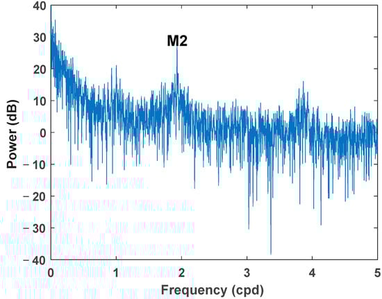
Figure 6.
Power spectrum of seawater temperature.
3.3. Current
The measurement data for ocean currents, selectively plotted to represent one month per season to avoid plot congestion, are shown in Figure 7. The analysis indicates that the currents in the south–north direction (v), where v is positive northward, are substantially stronger than those in the east–west direction (u), where u is positive eastward. Periodic fluctuations are observable in both u and v components, likely influenced by tidal forces due to the proximity of the ADCP measurement location to the coast. Particularly in the u component, there is an occasional reversal of flow direction between the upper and lower layers, suggesting the influence of baroclinic effects on the ocean currents.
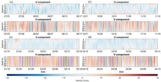
Figure 7.
Time series of ocean current in summer (a), autumn (b), winter (c), and spring (d). Only one month per season is plotted to avoid overcrowding the plot.
Statistical analysis of surface currents (at 3 m depth) is detailed in Table 3. The maximum speeds recorded in each season range from 63.10 cm s−1 to 71.89 cm s−1, with average speeds varying between 14.49 cm s−1 and 16.23 cm s−1. Notably, the mean speed in the v direction consistently exceeds that in the u direction, and the currents predominantly flow near the north–south direction.
Table 3.
Statistical analysis result of surface currents.
To elucidate the tidal influences on ocean currents, harmonic analysis was employed to characterize the tidal currents at each depth layer. Generally, the predominant tidal constituents include the M2 tide (principal lunar semidiurnal constituent), S2 tide (principal solar semidiurnal constituent), K1 tide (lunisolar diurnal constituent), and O1 tide (lunar diurnal constituent). Since the water depth of this instrument deployed is only 31 m, the current transferring water from deep water into shallow water may produce nonlinear effects due to the influence of topography. Figure 8a presents the tidal ellipses for these four main tidal constituents and the two largest tidal constituents outside these four tidal constituents measured at each layer over the entire measurement period. The M4 tide, a shallow water overtide of the principal lunar constituent, emerged as the strongest tidal current, followed by the M2 tide and then the MS4 tide, a shallow water quarter diurnal constituent. The M4 and MS4 tides are mainly nonlinear tides that are affected by the shallow water topography. Thus, the nonlinear effect of topography on ocean currents here is extremely significant. Furthermore, the orientation of the tidal currents predominantly aligns with nearly a north–south direction, but variations in the size and direction of tidal ellipses with depth indicate the presence of baroclinic effects.
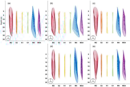
Figure 8.
Tidal ellipses for the main tidal constituents of each layer throughout the entire measurement time (a) and during summer (b), autumn (c), winter (d), and spring (e).
To assess seasonal variations, the current data were analyzed across distinct seasons: summer (June to August), autumn (September to November), winter (December to February), and spring (March to May). Figure 8b–e display the tidal ellipses of the four main tidal constituents and the M4 and MS4 tidal constituents in seasons. Consistently, the M4 tide dominated across all seasons, followed by the M2 and MS4 tides. While the ranking of tidal constituents remained stable, variations were noted in their magnitudes and directional orientations. To further dissect these differences, tidal currents were decomposed into barotropic and baroclinic components, providing deeper insights of their dynamic interactions and seasonal effects.
3.3.1. Barotropic Tidal Current
The barotropic tidal current is calculated by depth-averaging the raw current of each layer. The mean velocity is then analyzed by harmonic method to obtain the barotropic tidal constituents. The parameters defining the tidal current ellipse, semimajor axis (M), semiminor axis (m), inclination (ψ), phase (φ), and ellipticity (ε) are derived as follows. Initially, the amplitudes of east–west velocity (u) and north–south velocity (v), as well as the corresponding phases and of each tidal constituent, are analyzed through harmonic analysis. Subsequently, the tidal currents that change with time are decomposed by Equations (2) and (3) into the amplitudes of counterclockwise (CCW) component, , and clockwise (CW) component, , and their corresponding phases and by Equations (4) and (5) [,]:
After obtaining the amplitude and phase, the parameters of tidal current ellipse are calculated by Equations (6)–(10) as follows:
Figure 9 displays the tidal ellipses of barotropic currents for the four main tidal constituents (M2, S2, K1, and O1) derived from sea level, and the two larger tidal constituents (M4 and MS4) derived from ocean current. Table 4 lists the parameters of the barotropic tidal current constituents. Over the entire measurement period, the largest tidal constituent was the M4 tide, followed by the M2 and MS4 tides. The S2 tide and diurnal tides, such as the K1 and O1 tides, exhibited considerably smaller magnitudes. The inclination angles of the four major tidal constituents (M2, S2, K1, and O1) ranged between 88.52° and 97.76°, suggesting a predominantly north–south flow direction. However, the inclination angles of the M4 and MS4 tides exceeded 100°, indicating a slight deflection in the tidal currents due to topography influences, which introduce nonlinear behaviors. Additionally, the primary strong tidal current ellipses all rotate counterclockwise. Notably, the barotropic current associated with the M4 tide consistently exceeds that of the M2 tide, with this effect particularly pronounced in winter. This observation suggests the nonlinear effect of the M2 barotropic tidal force in winter, thereby intensifying the M4 barotropic tidal force.
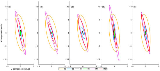
Figure 9.
Tidal ellipses for barotropic current in the M2, S2, K1, O1, M4, and MS4 tidal constituents throughout the entire measurement time (a), and in summer (b), autumn (c), winter (d), and spring (e).
Table 4.
Tidal ellipse parameters of barotropic current.
These results enhanced our understanding of the dynamics of barotropic tidal currents, particularly the significant seasonal variations and the influence of topographic effects. This provides valuable insights into the complex interactions that control tidal movements in the study area.
3.3.2. Baroclinic Tidal Current
Baroclinic tidal currents play an important role in ocean dynamics, affecting energy flux and mixing processes []. They can also cause harm to maritime structures because the upper and lower flow directions are inconsistent and may produce shear stress. Baroclinic tidal currents are primarily generated by the rise and fall of tides along the continental shelf and slopes, which significantly affect the distribution and circulation of water masses [].
Baroclinic tidal currents were calculated by subtracting the barotropic tidal currents from the raw time series data. Figure 10 illustrates the baroclinic tidal ellipses at various depth for six tidal constituents. Among these, the baroclinic tidal velocities of the O1, K1, S2, and MS4 tides are substantially lesser than those of the M2 and M4 tides throughout the entire measurement period. Therefore, the discussion here focuses primarily on the M2 and M4 tides. The M4 tidal current ellipse oriented in a northeast–southwest direction in the upper layer, aligning closer to a north–south direction in the lower layer. For the M2 tide, the orientation shifted from a northwest–southeast direction in the upper layer to a north–south direction in the lower layer. This directional disparity between layers creates nodal points, or zero-crossing depths, where no horizontal tidal motion occurs. Specifically, the zero-crossing depth of M2 tide is 18 m and that of M4 is 14 m, representing the first baroclinic mode of tidal currents.
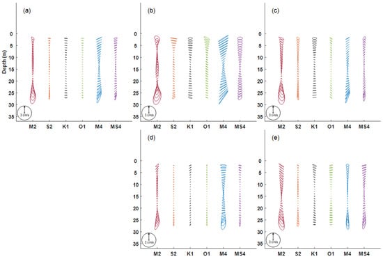
Figure 10.
The baroclinic tidal ellipses at each layer of six tidal constituents for the entire measurement period (a), summer (b), autumn (c), winter (d), and spring (e).
During the summer, the surface and bottom layers of the M4 tide exhibit the largest tidal ellipses, with the nodal depth situated around 14 m. The M2 tide shows the second-largest tidal ellipse with two nodal depths approximately at 7 m and 22 m. This pattern is distinct from other tidal constituents and seasons, as only the M2 tide in summer displays the second baroclinic mode. The sole CTD measurement, conducted during the recovery of the ADCP on 11 May 2024, supports this finding. Figure 11 depicts the seawater temperature profile measured by the CTD, revealing a temperature decrease from the surface down to 7 m, maintaining nearly constant temperatures between 7 and 22 m, and then a significant drop below 22 m. This temperature profile likely fosters the formation of internal tides at these depths. The dual nodal depths of the M2 tide’s second baroclinic mode coincide with the layers of temperature change, confirming that the occurrence of internal tides aligns with the thermocline layers. Although the CTD measurement was taken in mid-May, and summer in this study is defined from June to August, the conditions in mid-May already mirrored those typical of summer. In addition to the deep thermocline throughout the year in the waters of northeast Taiwan, a shallow thermocline forms from May to August due to the influence of strong solar radiation and the absence of northeast monsoon. Since the M2 tide is stronger, the second mode baroclinic tide may only appear in the M2 tide. The M4 tide is a nonlinear tide caused by the influence of topography on the M2 tide, so it may show different baroclinic node depths.
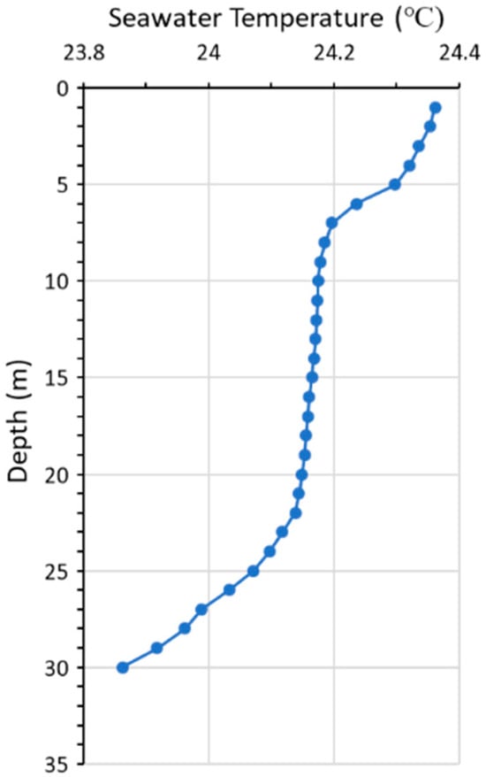
Figure 11.
Seawater temperature profile measured by CTD on 11 May 2024.
In other seasons, only the first baroclinic mode is evident. The node depths of the M2 and M4 tides are approximately 14 to 18 m. This situation may be due to the absence of dual thermoclines in seasons other than summer, resulting in a single nodal depth in the baroclinic tidal currents.
3.3.3. EOF Analysis
EOF analysis was employed to decompose baroclinic tidal currents into vertical variance modes and focused on the significant M2 and M4 tidal constituents. Figure 12 presents the decomposition results for the u and v components of these tidal currents. The first EOF mode for both u and v components of the M2 and M4 tides accounts for more than 90% of the total variability, except for the u component of the M2 tide during summer (75.2%) and winter (82.3%). In addition, except that the u component of the M2 tide in summer shows the baroclinic second mode tidal current, other seasons and components all show that the first baroclinic mode dominates.
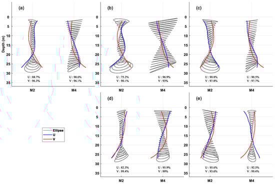
Figure 12.
EOF analysis of the first baroclinic mode of the M2 and M4 tides over the entire measurement period (a) and in summer (b), autumn (c), winter (d), and spring (e). The u component is in blue and the v component is in red, with the baroclinic tidal ellipses superimposed.
The structure of the first mode is typical in continental shelf waters [,]. The sea area of this study is the shallow water coast near the mouth of the bay, and the same phenomenon can also be observed. The results of the EOF analysis are superimposed on the baroclinic tidal ellipse obtained by subtracting the depth-averaged ocean currents. It is clearly seen that the nodes of the baroclinic tidal flow ellipse are closely aligned with the zero crossing of the u component. This arrangement shows that the dominant baroclinic effect originates from the east–west component of the tidal current, highlighting the directional influence of topographic features on tidal dynamics in the region.
3.3.4. Rotary Spectra
Rotary spectral analysis is a method used to identify the primary rotational patterns in ocean currents. It helps determine the direction of flow, whether it is clockwise or counterclockwise. Understanding the flow dynamics in various maritime habitats is crucial []. Tidal currents in the open oceans of the Northern Hemisphere often flow in a clockwise direction due to the influence of the Earth’s rotation. Nevertheless, the configuration of the continental shelf can also influence the direction of tidal currents. Due to the position of the ADCP deployment close to the coast, the tidal currents are significantly influenced by the topography. The objective of conducting rotational spectral analysis is to comprehend the flow orientation of various tidal currents at different depths. This could offer additional insights into the impact of ocean currents on the reliability and security of wave energy devices deployed in this region.
Figure 13 depicts the outcome of the rotary spectra of depth-averaged currents. The spectral power of the inertial frequency, f, is lower compared to the major tidal constituents. This indicates that the Earth’s rotation has little influence on ocean currents in this area, while tides play a significant role. In comparison to other frequencies, the spectral powers of the semidiurnal tidal constituents (M2 and S2) and their overtides (M4 and MS4) are greater, and the CCW power spectra of the four tidal constituents are slightly higher than the CW power. Figure 14 shows the CW and CCW spectra for the four tidal constituents from sea surface to bottom, which were used to investigate the rotational orientations of baroclinic tides. Throughout the entire measurement period, as illustrated in Figure 14a, the CCW spectrum shows that the M2 tide has the highest power, followed by the M4 tide, with the S2 tide exhibiting the lowest power. However, the CW spectrum shows that M4 has the highest power, M2 and MS4 powers are approximately equal, and S2 has the lowest power. The CCW power of the M4 tide and MS4 tide is almost the same as the CW power, but the CCW power of the M2 tide and S2 tide is much larger than the CW power.
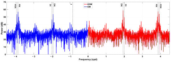
Figure 13.
The power spectrum of surface current.
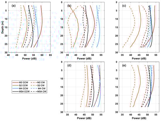
Figure 14.
Rotary spectra for counterclockwise (CCW, solid line) and clockwise (CW, dashed line) in the frequencies of M2, S2, M4, and MS4 tidal constituents throughout the entire measurement time (a), in summer (b), autumn (c), winter (d), and spring (e).
To discern seasonal variations, rotary spectra for each season were analyzed. Figure 14b–e display the rotary spectra across the four seasons. In summer (Figure 14b), the M4 tide displays the largest CCW power, followed by the M2, S2, and MS4 tides, with a similar pattern observed in the CW power. However, the CW power for the M4 and S2 tides surpasses the CCW power at the surface layer, whereas for other tides, CCW power predominates across all depths.
In autumn, shown in Figure 14c, the CCW power is greatest for the M2 tide, with the M4 and MS4 tides exhibiting nearly equal power, and the S2 tide the least. For the CW power, the M4 tide has the largest power, followed by the MS4 tide, with the S2 tide showing the smallest power. Generally, CCW power exceeds CW power, except in the surface layer for the M4 tide where CW power is marginally higher.
Winter results, displayed in Figure 14d, indicate that CCW power for the M2 tide slightly outstrips that of the M4 tide in the upper layer (shallower than 12 m), but below this depth, the M4 tide’s power is greater. The MS4 tide’s CCW power ranks below the M2 and M4 tides, with the S2 tide showing the least power. For CW power, the M4 tide is the largest, the M2 tide is close to the MS4 tide, and the S2 tide is the smallest. However, at depths below 10 m, the CCW power of the M4 tide is greater than the CW power. MS4 tides have a similar situation, but the depth is different, about 7 m.
Spring spectra, as seen in Figure 14e, reveal that the CCW power of the M2 tide is the largest above 20 m, followed by the M4 and MS4 tides, with the S2 tide remaining the smallest. Below 20 m, the CCW power of the M4 and MS4 tides is nearly identical, and the M2 tide shows slightly lesser power. For CW power, the M4 tide is the largest, the M2 tide is close to the MS4 tide, and the S2 tide is the smallest. However, at depths below 10 m, the CCW power of the M4 tide is greater than the CW power. MS4 tides have a similar situation, but the depth is different, about 7 m.
Generally, CW power is expected to be more pronounced in the Northern Hemisphere than CCW power due to the Earth’s rotation. However, the results of this study suggest otherwise. This is most likely due to the influence of coastal topography and the bay’s configuration, which disrupt the typical propagation direction of tidal currents in an open ocean environment. According to the literature [], an analysis was conducted on the rotary spectra of ocean currents measured at a mooring station situated on the continental slope in northeastern Taiwan (25°30.3′ N, 122°35.8′ E, 600 m sea depth). The research reveals that the CW component exhibits a greater spectral energy compared to the CCW component, both in inertial frequency and major tidal frequencies. This is similar to results obtained in the open ocean, meaning that it is unaffected by the seafloor. The findings in this study are significantly different from theirs. Although both study areas are located in the waters northeast of Taiwan, there is a considerable difference in water depths. It is evident that the ocean currents in this study area are strongly influenced by the seafloor.
As stated in Section 3.2, strong tidal currents flow northwest–southeast parallel to the bay mouth. These tidal currents produce relatively slow cyclonic and anticyclonic circulations within the bay during flood and ebb tides, respectively. Since the ADCP position is close to the left side of the bay mouth, the current velocity at the ADCP position during flood tide is affected by the faster tidal current outside the bay that has just entered the bay. Instead, during the ebb tide, it is affected by the slower circulation within the bay. This is likely why the CCW power was slightly larger than the CW power in this study.
4. Conclusions
This study used a bottom-mounted acoustic Doppler current profiler (ADCP) to measure current profiles in coastal waters near the wave energy instrument test area over nearly a year. The main objective is to assess whether ocean currents pose a risk to the operational integrity of the test equipment. In addition to analyzing ocean currents, ADCP records sea surface height and seawater temperature at instrument depth. Data analysis shows that water level changes in this area are mainly affected by the M2 tide, followed by the O1 tide, K1 tide, and S2 tide. Changes in seawater temperature are also affected by tides, especially the M2 tide. The typhoon passing from southern Taiwan can cause the maximum cooling effect to be close to 10 °C.
The strongest measured current speed is about 72.0 cm s−1, and the average speed is about 15.5 cm s−1. The average flow direction is approximately north–south. The largest tidal current is the M4 tide, followed by the M2 tide. The semimajor axis and inclination angle of the barotropic tidal ellipse of the M4 and M2 tides are 8.48 cm s−1 and 102.60°, and 7.00 cm s−1 and 97.76°, respectively, and these tidal currents show maximum intensity in winter. As for the baroclinic tidal current, it is calculated using the depth-average method, with the first baroclinic mode being the main one, and the zero-crossing depth being 14 to 18 m. It is worth noting that the M2 baroclinic tidal current exhibits a second baroclinic mode in summer, which is characterized by two zero-crossing depths of approximately 7 m and 22 m, respectively. These findings are consistent with those obtained from EOF analysis.
Internal tidal currents exist in shallow water near the coast. Although these currents are not particularly strong, opposing flow directions between the surface and bottom layers may still pose a risk to moored wave energy devices, particularly due to the potential for increased mechanical stress on the mooring cables. The results of this study provided an evaluation of the magnitude of risk and probability of occurrence in the future.
Author Contributions
Conceptualization, C.-R.H. and T.-W.H.; methodology, C.-R.H.; software, K.-H.C.; validation, C.-R.H., Z.-W.Z. and H.-J.L.; formal analysis, K.-H.C.; investigation, C.-R.H.; resources, T.-W.H.; data curation, C.-R.H.; writing—original draft preparation, C.-R.H. and K.-H.C.; writing—review and editing, C.-R.H., Z.-W.Z. and H.-J.L.; visualization, K.-H.C.; supervision, C.-R.H. and T.-W.H.; project administration, T.-W.H.; funding acquisition, C.-R.H. and T.-W.H. All authors have read and agreed to the published version of the manuscript.
Funding
This research was funded by National Science and Technology Council of Taiwan, grant number NSTC 111-2611-M-019-017-MY3 and NSTC 113-2218-E-019-011.
Institutional Review Board Statement
Not applicable.
Informed Consent Statement
Not applicable.
Data Availability Statement
The data presented in this study are available on request from the corresponding author.
Acknowledgments
The authors thank the anonymous reviewers for their constructive comments and suggestions.
Conflicts of Interest
The authors declare no conflicts of interest.
References
- Gibson, L.; Wilman, E.N.; Laurance, W.F. How green is ‘green’ energy? Trends. Ecol. Evol. 2017, 32, 922–935. [Google Scholar] [CrossRef]
- Panwar, N.L.; Kaushik, S.C.; Kothari, S. Role of renewable energy sources in environmental protection: A review. Renew. Sustain. Energy Rev. 2011, 15, 1513–1524. [Google Scholar] [CrossRef]
- Arent, D.J.; Wise, A.; Gelman, R. The status and prospects of renewable energy for combating global warming. Energy Econ. 2011, 33, 584–593. [Google Scholar] [CrossRef]
- Sher, F.; Curnick, O.; Azizan, M.T. Sustainable conversion of renewable energy sources. Sustainability 2021, 13, 2940. [Google Scholar] [CrossRef]
- Voigt, C. Oceans and Climate Change: Implications for UNCLOS and the UN Climate Regime. In The Environmental Rule of Law for Oceans: Designing Legal Solutions; Platjouw, F.M., Pozdnakova, A., Eds.; Cambridge University Press: Cambridge, UK, 2023; pp. 17–30. [Google Scholar]
- Lehmann, M.; Karimpour, F.; Goudey, C.A.; Jacobson, P.T.; Alam, M.R. Ocean wave energy in the United States: Current status and future perspectives. Renew. Sustain. Energy Rev. 2017, 74, 1300–1313. [Google Scholar] [CrossRef]
- Veerabhadrappa, K.; Suhas, B.G.; Mangrulkar, C.K.; Kumar, R.S.; Mudakappanavar, V.S.; Seetharamu, K.N. Power generation using ocean waves: A review. Glob. Trans. Proc. 2022, 3, 359–370. [Google Scholar] [CrossRef]
- Gelfenbaum, G. Coastal currents. In Encyclopedia of Coastal Science; Schwartz, M.L., Ed.; Springer: Dordrecht, The Netherlands, 2005; pp. 259–260. [Google Scholar]
- Klemas, V. Remote sensing of coastal and ocean currents: An overview. J. Coast. Res. 2012, 28, 576–586. [Google Scholar] [CrossRef]
- Li, M.; Rong, Z. Effects of tides on freshwater and volume transports in the Changjiang River plume. J. Geophys. Res. Oceans 2012, 117, C06027. [Google Scholar] [CrossRef]
- Munk, W.; Wunsch, C. Abyssal recipes II: Energetics of tidal and wind mixing. Deep-Sea Res. I Oceanogr. Res. Pap. 1998, 45, 1977–2010. [Google Scholar] [CrossRef]
- Egbert, G.D.; Ray, R.D. Significant dissipation of tidal energy in the deep ocean inferred from satellite altimeter data. Nature 2000, 405, 775–778. [Google Scholar] [CrossRef]
- Baines, P.G. On internal tide generation models. Deep-Sea Res. I Oceanogr. Res. Pap. 1982, 29, 307–338. [Google Scholar] [CrossRef]
- Garrett, C.; Kunze, E. Internal tide generation in the deep ocean. Annu. Rev. Fluid Mech. 2007, 39, 57–87. [Google Scholar] [CrossRef]
- Subeesh, M.P.; Unnikrishnan, A.S.; Fernando, V.; Agarwadekar, Y.; Khalap, S.T.; Satelkar, N.P.; Shenoi, S.S.C. Observed tidal currents on the continental shelf off the west coast of India. Cont. Shelf Res. 2013, 69, 123–140. [Google Scholar] [CrossRef]
- Zaron, E.D. Internal tides. In Encyclopedia of Ocean Sciences, 3rd ed.; Cochran, J.K., Bokuniewicz, H.J., Yager, P.L., Eds.; Academic Press: Cambridge, MA, USA, 2019; pp. 633–641. [Google Scholar]
- Rattray, M., Jr. On the coastal generation of internal tides. Tellus 1960, 12, 54–62. [Google Scholar] [CrossRef]
- Shepard, F.P. Progress of internal waves along submarine canyons. Mar. Geol. 1975, 19, 131–138. [Google Scholar] [CrossRef]
- Duda, T.F.; Lynch, J.F.; Irish, J.D.; Beardsley, R.C.; Ramp, S.R.; Chiu, C.S.; Tang, T.Y.; Yang, Y.J. Internal tide and nonlinear internal wave behavior at the continental slope in the northern South China Sea. IEEE J. Ocean. Eng. 2004, 29, 1105–1130. [Google Scholar] [CrossRef]
- Pawlowicz, R.; Beardsley, B.; Lentz, S. Classical tidal harmonic analysis including error estimates in MATLAB using T_TIDE. Comput. Geosci 2002, 28, 929–937. [Google Scholar] [CrossRef]
- Wang, Y.; Zhang, Y.; Wang, J.; Lv, X. The essential observations for reconstructing full-depth tidal currents. Front. Mar. Sci. 2022, 9, 959014. [Google Scholar] [CrossRef]
- Bravo, L.; Ramos, M.; Sobarzo, M.; Pizarro, O.; Valle-Levinson, A. Barotropic and baroclinic semidiurnal tidal currents in two contrasting coastal upwelling zones of Chile. J. Geophys. Res. Oceans 2013, 118, 1226–1238. [Google Scholar] [CrossRef]
- Edwards, C.R.; Seim, H.E. Complex EOF analysis as a method to separate barotropic and baroclinic velocity structure in shallow water. J. Atmos. Ocean. Technol. 2008, 25, 808–821. [Google Scholar] [CrossRef]
- López, M.; Flores-Mateos, L.; Candela, J. Tidal currents at the sills of the Northern Gulf of California. Cont. Shelf Res. 2021, 227, 104513. [Google Scholar] [CrossRef]
- Jithin, A.K.; Unnikrishnan, A.S.; Fernando, V.; Subeesh, M.P.; Fernandes, R.; Khalap, S.; Narayan, S.; Agarvadekar, Y.; Gaonkar, M.; Kankonkar, A.; et al. Observed tidal currents on the continental shelf off the east coast of India. Cont. Shelf Res. 2017, 141, 51–67. [Google Scholar] [CrossRef]
- Li, M.; Xie, L.; Zong, X.; Li, J.; Li, M.; Yan, T.; Han, R. Tidal currents in the coastal waters east of Hainan Island in winter. J. Oceanol. Limnol. 2022, 40, 438–455. [Google Scholar] [CrossRef]
- Kaihatu, J.M.; Handler, R.A.; Marmorino, G.O.; Shay, L.K. Empirical orthogonal function analysis of ocean surface currents using complex and real-vector methods. J. Atmos. Ocean. Technol. 1998, 15, 927–941. [Google Scholar] [CrossRef]
- Hall, P.; Davies, A.M. Analysis of time-varying wind-induced currents in the North Channel of the Irish Sea, using empirical orthogonal functions and harmonic decomposition. Cont. Shelf Res. 2002, 22, 1269–1300. [Google Scholar] [CrossRef]
- Kuo, N.J.; Ho, C.R. ENSO effect on the sea surface wind and sea surface temperature in the Taiwan Strait. Geophys. Res. Lett. 2004, 31, L13309. [Google Scholar] [CrossRef]
- Tseng, Y.H.; Lu, C.Y.; Zheng, Q.; Ho, C.R. Characteristic analysis of sea surface currents around Taiwan island from CODAR observations. Remote Sens. 2021, 13, 3025. [Google Scholar] [CrossRef]
- Zheng, Z.W.; Chen, Y.R. Influences of tidal effect on upper ocean responses to typhoon passages surrounding shore region off northeast Taiwan. J. Mar. Sci. Eng. 2022, 10, 1419. [Google Scholar] [CrossRef]
- Kristensen, L.; Christiansen, H.H.; Caline, F. Temperatures in coastal permafrost in the Svea area, Svalbard. In Proceedings of the Ninth International Conference on Permafrost, Fairbanks, AK, USA, 3–28 June 2008. [Google Scholar]
- Kim, T.W.; Cho, Y.K.; You, K.W.; Jung, K.T. Effect of tidal flat on seawater temperature variation in the southwest coast of Korea. J. Geophys. Res. 2010, 115, C02007. [Google Scholar] [CrossRef]
- Hsu, P.C.; Lee, H.J.; Zheng, Q.; Lai, J.W.; Su, F.C.; Ho, C.R. Tide-induced periodic sea surface temperature drops in the coral reef area of Nanwan Bay, southern Taiwan. J. Geophys. Res. Oceans 2020, 125, e2019JC015226. [Google Scholar] [CrossRef]
- Asplin, L.; Lin, F.; Budgell, W.P.; Strand, Ø. Rapid water temperature variations at the northern shelf of the Yellow Sea. Aquac. Environ. Interact. 2021, 13, 111–119. [Google Scholar] [CrossRef]
- Chen, K.; Huang, C.F.; Zheng, Z.W.; Lin, S.F.; Liu, J.Y.; Guo, J. Optimum estimation of coastal currents using moving vehicles. J. Atmos. Ocean. Technol. 2023, 40, 1619–1629. [Google Scholar] [CrossRef]
- Godin, G. The Analysis of Tides; University of Toronto Press: Toronto, ON, Canada, 1972; 264p. [Google Scholar]
- Pu, X.; Shi, J.Z.; Hu, G.D. The effect of stratification on the vertical structure of the tidal ellipse in the Changjiang River estuary, China. J. Hydroenviron. Res. 2017, 15, 75–94. [Google Scholar] [CrossRef]
- Yan, T.; Qi, Y.; Jing, Z.; Cai, S. Seasonal and spatial features of barotropic and baroclinic tides in the northwestern South China Sea. J. Geophys. Res. Oceans 2020, 125, e2018JC014860. [Google Scholar] [CrossRef]
- Zaron, E.D.; Musgrave, R.C.; Egbert, G.D. Baroclinic tidal energetics inferred from satellite altimetry. J. Phys. Oceanogr. 2022, 52, 1015–1032. [Google Scholar] [CrossRef]
- Shearman, R.K. Observations of near-inertial current variability on the New England shelf. J. Geophys. Res. Oceans 2005, 110, C02012. [Google Scholar] [CrossRef]
- Wang, Z.; Li, Q.; Wang, C.; Qi, F.; Duan, H.; Xu, J. Observations of internal tides off the coast of Shandong Peninsula, China. Estuar. Coast. Shelf Sci. 2020, 245, 106944. [Google Scholar] [CrossRef]
- Chandna, S.; Walden, A.T. Statistical properties of the estimator of the rotary coefficient. IEEE Trans. Signal Process. 2010, 59, 1298–1303. [Google Scholar] [CrossRef][Green Version]
- Yin, Y.; Liu, Z.; Zhang, Y.; Chu, Q.; Liu, X.; Hou, Y.; Zhao, X. Internal tides and their intraseasonal variability on the continental slope northeast of Taiwan island derived from mooring observations and satellite data. Remote Sens. 2021, 14, 59. [Google Scholar] [CrossRef]
Disclaimer/Publisher’s Note: The statements, opinions and data contained in all publications are solely those of the individual author(s) and contributor(s) and not of MDPI and/or the editor(s). MDPI and/or the editor(s) disclaim responsibility for any injury to people or property resulting from any ideas, methods, instructions or products referred to in the content. |
© 2024 by the authors. Licensee MDPI, Basel, Switzerland. This article is an open access article distributed under the terms and conditions of the Creative Commons Attribution (CC BY) license (https://creativecommons.org/licenses/by/4.0/).