Analyzing Social Media Data Using Sentiment Mining and Bigram Analysis for the Recommendation of YouTube Videos

Abstract

In this work we combine sentiment analysis with graph theory to analyze user posts, likes/dislikes on a variety of social media to provide recommendations for YouTube videos. We focus on the topic of climate change/global warming, which has caused much alarm and controversy over recent years. Our intention is to recommend informative YouTube videos to those seeking a balanced viewpoint of this area and the key arguments/issues. To this end we analyze Twitter data; Reddit comments and posts; user comments, view statistics and likes/dislikes of YouTube videos. The combination of sentiment analysis with raw statistics and linking users with their posts gives deeper insights into their needs and quest for quality information. Sentiment analysis provides the insights into user likes and dislikes, graph theory provides the linkage patterns and relationships between users, posts, and sentiment.

1. Introduction

Recommender systems (RS) are intended to provide the online user with advice, reviews, and opinions from previous purchasers on products and services mainly through methods such as collaborative filtering (CF) [1]. The main RS objective using CF is to persuade users to buy items or services they have not previously bought/seen before based on the buying patterns of others. This can be achieved by ranking either the item-to-item similarity or the user-to-user similarity and then predicting the top scoring product that ought to appeal to the potential buyer. Unfortunately, CF has a number of limitations such as the cold-start problem, i.e., generating reliable recommendations for those with few ratings or items. However, this issue can be alleviated to some extent by reusing pre-trained deep learning models and/or using contextual information [2]. Since CF is generally an open process, they can be vulnerable to biased information or fake information [3,4]. Fake user profiles can easily manipulate recommendation results by giving the highest rates to targeted items and rate other items similar to regular profiles. This behavior is called a “shilling attack” [5].

Initially launched in 2005, YouTube has seen an exponential growth of submitted videos and is the most popular platform for viewing material that informs, educates, and entertains its users. YouTube is a free video sharing service allowing users to view online videos and also for them to develop and upload their own materials to share with others [6,7]. However, for many YouTube contributors the opportunity to earn money from their channel’s popularity is a great incentive. To earn money from YouTube, a contributor must have 1000 subscribers and at least 4000 watch hours in the past year. Contributors can then apply to YouTube’s Partner Program and monetize their channel. However, YouTube keeps careful surveillance on any mechanism that artificially inflates the number of comments, views, or likes. Unscrupulous contributors often achieve increased rankings by using bots or automatic systems or even presenting videos to unsuspecting viewers.

The objective of our work is to demonstrate that a recommendation engine can be used to provide users with reliable YouTube videos based on initial keyword searches. The topic of interest is global warming/climate change, but the system could be applied to any subject. The objectives are two-fold: once we can identify their sentiment/opinions on global warming we can provide users with authoritative videos with scientific credence based on their beliefs. Then, we can present users with authoritative videos representing the opposite stance. The intent is to balance out the debate with evidence that they would perhaps not necessarily seek out. Our intention is not to change opinions, but to help users become more aware of the issues.

To achieve these objectives, we combine sentiment analysis and graph theory to provide deeper insights into YouTube recommendations. Rather than using different software platforms, we combine several R libraries into a unified system, making overall integration easier. The overall system workflow is shown in Figure 1. An initial search topic is defined and fed into the APIs of the three platforms (Twitter, Reddit, and YouTube). The resulting posts are preprocessed and parsed, and the text data is then analyzed by graph theoretic measures that provide statistical metrics of user posts and how they interact. The sentiments of user posts are used to create topic maps that reflect common themes and ideas that these users have. Ratings of YouTube videos and the provenance of their sources are estimated to provide some indication of their validity and integrity.

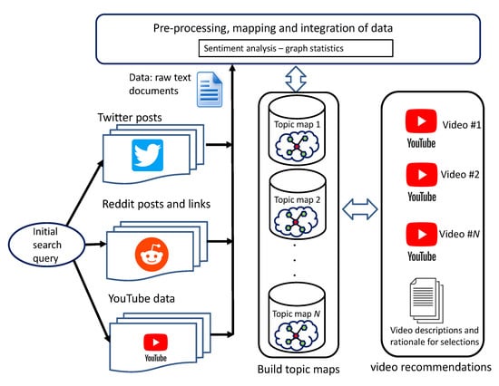
Figure 1. Overall system operation of data throughput and transformations.

The main contribution of this work is three-fold. First we integrate sentiment mining with graph theory, providing statistical information on the posters and contributors. We also use up-votes and down-votes as a recommendation source. Finally we create a logical structuring of the Twitter, Youtube, and Reddit data using topic maps. Topic modellng is necessary since most topics of interest will comprise a mixture of words and sentiments, which is a feature of human language. Therefore, some overlapping of concepts will occur, so an unsupervised classification method is required. We use Latent Dirichlet allocation (LDA), which is commonly used for fitting a topic model [8].

The remainder of this paper is structured as follows: Section 2 describes the related work and recent advances in recommender systems. Section 3 outlines the social media data used in this study. Section 4 describes the computational methods used. Section 5 presents the experimental results and the discussion. Finally, Section 6 presents the conclusions and future work.

2. Related Work

Here we discuss related work for recommender systems, sentiment analysis, and graph theoretic methods.

2.1. Recommender Systems

We can say that recommender systems can be categorized into three main groups: content-based recommender systems, collaborative recommender systems, and hybrid recommender systems. One of the first and most predominant is the Amazon recommendation system, which has undergone many refinements over the past 20 years [9]. The RS are generally trained from historical data and provide the customer with potentially useful feedback with products or services that they may like. The details of the RS algorithm used by YouTube is unknown, but it is generally believed to employ deep neural learning [10]. However, a recent study revealed it to contain biases and being a major source of misinformation on certain health related videos [11]. Another issue, which we do not tackle in this paper, are the attacks on recommender systems to either down vote or up vote content [12].

Our system can be classed as a hybrid. Similar work to ours includes the study of Kim and Shim, who proposed a recommender system based on Latent Dirichlet Allocation (LDA) using probabilistic modeling for Twitter [13]. The top-K tweets for a user to read along with the top-K users that should be followed are identified based on LDA. The Expectation–Maximization (EM) algorithm was used to learn model parameters. Abolghasemi investigated the issues around human personality in decision-making as it plays a role when individuals discuss how to reach a group decision when deciding which movie to watch [14]. They devised a three-stage approach to decision making, and used binary matrix factorization methods in conjunction with an influence graph that includes assertiveness and cooperativeness as personality traits. They then applied opinion mining to reach a common goal. We use similar metrics to judge personalities based on the tenor/tone of language used and their likes and dislikes.

A similar approach was taken by Leng et al. who were researching social influence and interest evolution for group recommendations [15]. The system they developed (DASIIE) is designed to dynamically aggregate social influence diffusion and interest evolution learning. They used Graph Neural Networks as the basis of their recommendation system. The neural network approach allowed them to integrate the role weights and expertise weights of the group members, enabling the decision-making process to be modeled simultaneously. Wu et al. have examined the technique of data fusion for increasing the efficiency of item recommender systems. It employed a hybrid linear combination model and used a collaborative tagging system [16].

2.2. Sentiment Analysis

Over the past 10 years or so sentiment analysis has seen a massive expansion both in practical applications and research theory [17,18,19]. The process of sentiment mining involves the preprocessing of text by using either simple text analytics or a more complex NLP, such as the Stanford system [20]. The text data can be organized by individual words or at the sentence and paragraph level depending on the positive or negative words it comprises [21]. Words are deemed to be either neutral, negative, or positive based on the assessment of a lexicon [22,23]. Sentiment analysis is employed in many different areas from finance [24,25] to mining student feedback in educational domains [26,27]. It has also been used to automatically create ontologys from text [28]. Sentiment analysis has been used to examine the satisfaction within the computer gaming community, observing features in games that the players liked/disliked [29]. We have seen commercial applications for the automated mining of customer emails/feedback/reviews for improving satisfaction with products or services, which is a field that has seen tremendous growth [30,31]. Twitter is often used as a source of data for sentiment mining on many topics [32]. In particular, Tweets collected over long time periods tend to reveal interesting trends and patterns [33]. For example, sentiment analysis has been applied to monitoring mental health issues based on Tweets [34].

The study by Kavitha is similar to ours as it considered YouTube user comments based on their relevance to the video content given by the description [35]. The authors built a classifier that analyzed heavily liked and disliked videos. Similarly, we use counts to help rate the videos. They also considered spam and malicious content, and we also filter out posts that contain sarcastic and profane content as they are unlikely to contain much cogent information [11]. A more serious issue was considered by Abul-Fottouh in the search for bias in YouTube vaccination videos. They discovered that pro-vaccine videos (64.75%) outnumbered anti-vaccine (19.98%) videos with perhaps 15.27% of videos being neutral in sentiment. It is unsurprising that YouTube tended to recommend neutral and pro-vaccine videos rather than anti-vaccine videos. This implies that YouTube’s recommender algorithm will recommend similar content to users with similar viewing habits and similar comments. This is related to the sentiment work of Alhabash who investigated cyber-bullying on YouTube. This involved examining comments, virality, and arousal levels on civic behavioral patterns [36]. The findings concluded that people are more committed/interested in topics or comments that have negative sentiments, hence cyber-bulling videos appear to have a disproportionate effect on users. Further work by Shiryaeva et al. investigated the negative sentiment (anti-values) in YouTube videos. Here the viewpoint was taken from the lens of linguistics to reveal grammar and style indicative of certain behaviors and intentions [37]. Although the work was not automated, the authors were able to identify 12 anti-values that were characteristic of bad behavior.

2.3. Graph Theory

This area of computer science uses statistical measures to gather information about the connectivity patterns between the nodes (which can be people, objects, or communications) which can reveal useful insights into the dynamics, structure, and relationships that may exist [38,39]. Numerous areas have benefited from graph theory such as computational biology and especially social media, which has received a great deal of attention from researchers [40]. The most notorious incident was the FaceBook/Cambridge Analytica scandal, which involved the misuse of personal data [41]. However, this particular case served to highlight the power of machine learning and interconnected data to influence individuals. In social media analysis, individuals are connected to friends, colleagues, political, financial, and personal web interests, all of which can be analyzed by organizations to improve services and products or detect trends and opinions [42].

Graph theory was used by Cai to examine the in-degree of posters. Their intention was to identify if Schilling attacks were occurring in user posts [43]. Each user was assigned a “suspicion” rating based on their in-degree and their behavior characteristics such as diversity of interests, long-term memory of interest, and memory of rating preference. The graph information was fed to a density clustering method and malicious users were generally identified. A similar approach was taken by Cruickshank to use a combination of graph theory and clustering on Twitter hash-tags [44]. The method investigated the application of multiple different data types that can be used to describe how users interact with hashtags on the COVID-19 Twitter debate. They discovered that certain topical clusters of hashtags shifted over the course of the pandemic, while others were more persistent. The same effect (homophilly) is likely to be true of the climate change debate. For example, the HarVis system of Ahmed uses graph theory to untangle frequent from infrequent posters to gain a better understanding of the authors/posters ranking [45]. This is an important point, as it is best to weigh authoritative heads instead of just counting them.

The use of graph-like structures such as Graph Convolutional Networks (GCN) is becoming more popular. This approach has the flexibility and power to model many social media problems. These are more powerful than standard graph theoretic methods but come with a computational burden and requirement for more data. The use of GCN is also receiving attention for identifying Schilling attacks in recommender systems [46]. Another issue is the informal language used in posts and other characteristics of this type of data. For example, Keramatfor et al. found that short posts such as Tweets have dependencies upon previous posts [47,48]. Modeling Tweet dependencies requires the combination of data such as textual similarity, hashtag usage, sentiment similarity, and friends in common.

In Table 1 we provide a short qualitative comparison with the most similar recommendation systems to ours. The difference is that our system uses a greater variety of social media data and uses profiling and a wider variety of computational methods.

Table 1. Qualitative comparison with other systems.

Author	System Name	Date	Methods	Social Media
McGarry			Graph theory, sentiment analysis, bigrams, profiling	Twitter, YouTube, reddit
Keramatfar [47]	MHLSTM	2021	LSTM, profiling, sentiment analysis	Twitter
Cruickshank [44]	MVMC	2020	Hash-tags, sentiment analysis	Twitter
Ahmad [45]	HarVis	2017	Graph theory	YouTube
Kavitha [35]		2020	Bag of Words, NLP	YouTube
Kim [13]	TWLITE	2014	LDA, probability	Twitter
Nilashi [49]		2023	LDA, EM, clustering	TripAdvisor

3. Data

Here we describe our data sources, how they are pre-processed and integrated prior to building machine learning models and implementing the recommendation system. Twitter, Reddit, and Youtube posts are searched based on climate change keywords, then downloaded using the appropriate APIs, and the posts are cleaned of stop words, stemming, punctuation and emojis. A separate corpus, consisting of a term-document-matrix, is created for each data source. We then build topic maps for each corpus. The optimum number is generated from a range of 10–100 potential topics. The most optimum number is selected by calculating the harmonic mean for each number. We did not analyze the social media data to determine if any content was generated by bots. The social media companies are well aware of the issues and have developed bot detection software [50,51] for a comprehensive recent survey, see Hayawi et al. [52].

In Table 2 the sources of the data are presented, showing the number of the records, the approximate date of collection, and where they are collected from.

Table 2. Data sources, number of records, and approximate date of collection.

Data	Source	Date	No Records
Twitter	API	January 2020 to March 2020	2K
Twitter	Kaggle	April 2015 to February 2018	44K
Reddit	API	December 2022 to February 2023	100K
YouTube	API	December 2022 to February 2023	26K

3.1. Reddit Data

Reddit is a social news aggregation platform and discussion forum where users can post comments, web links, images, and videos. Other users can up/down vote these posts and engage in dialog. The site is well known for its open and diverse nature. User posts are organized by subject into specific boards called communities or subreddits. The communities are moderated by volunteers who set and enforce rules specific to a given community. They can remove posts and comments that are offensive or break the rules, and also keep discussions on the subject topic [53,54,55]. Reddit is becoming very popular as shown statistics from the SemRush web traffic system, which estimates Reddit to be the 6th most visited site in the USA [56]. In this study, we text-mine Reddit for posts and sentiment pertaining to the issues surrounding the climate change debate [57,58,59,60,61]. The Reddit data was collected between December 2022 and February 2023. Due to rate limits imposed by the Reddit API, we utilized the R interface (RedditExtractoR) for data extraction [62].

The Reddit data consists of two structures: the comments and the threads. The comments data consists of the following variables: URL, author, date, timestamp, score, upvotes, downvotes, golds, comment, and the comment-id. The threads data has further information pertaining to other user actions on the posts such as total-awards-received, golds, cross-posts, and other user comments. Figure 2 shows a list of the types of data residing in the posts.

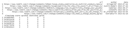
Figure 2. Preprocessed Reddit data structure.

3.2. YouTube Data

Youtube provides data pertaining to user opinions on the various videos they find of interest. Figure 3 displays a data structure showing the first 10 records of Youtube data. The Comment column is the user post, other columns identify the user ID, authors image profile URL, author channel ID, author channel URL, reply count, like count, post published date, when post updated, post parent ID, post ID, and video ID. The Youtube data was collected December 2022 and February 2023 using the R vosonSML package [63].

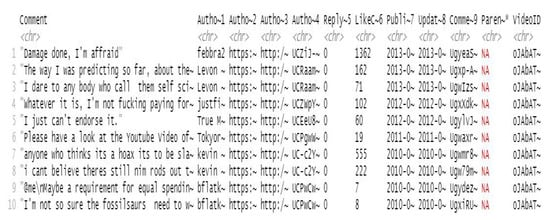
Figure 3. Preprocessed Youtube data structure.

3.3. Twitter Data

The data downloaded and preprocessed from Twitter consisted of two sources. Twitter was more problematic as difficulties were encountered recently with the API access. The first set of data was collected by API by the authors in 2020 and then from a datasource in the public domain from Kaggle. This consisted of 44,000 tweets collected by the University of Waterloo in 2015–2018 [64]. Twitter contains variables similar to Reddit and Youtube as they describe the UserScreenName, the UserName, the Timestamp, Text, Embedded-text, Emojis, Comments, Like counts, number of Retweets, Image.links and the Tweet.URL. This is displayed in Figure 4.

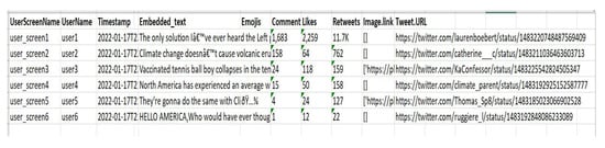
Figure 4. Preprocessed Twitter data structure.

4. Methods

In Figure 5 the basic flow of social media searching, storage of data, and flow information is presented. This example is for global warming/climate change, but the process would be similar for any topic of interest e.g., the war in Ukraine or the COVID pandemic. Keywords are selected and used to search the social media, and YouTube videos are downloaded and observed for validity. The data is saved in RDATA format (R programming language format). The data structures are formed from sentiment, graph analysis of bigrams, and user profiles consisting of likes/dislikes and overall estimated stance on global warming. Data are split for training 90% and 10% for test. The recommendation engine is constructed and tested and compared with other methods.

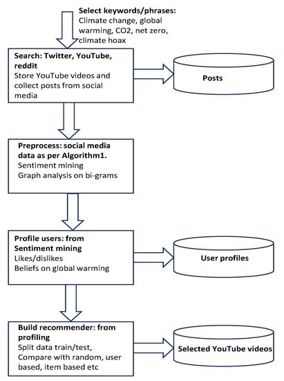
Figure 5. Data collection, storage, and processing.

The three datasets from Twitter, YouTube, and Reddit must now be preprocessed prior to sentiment analysis. In Algorithm 1 we show the stages of processing the three data sources (Twitter ${\mathbf{T}}_{\mathbf{txt}}$, Reddit ${\mathbf{R}}_{\mathbf{txt}}$, and ${\mathbf{Y}}_{\mathbf{txt}}$ YouTube). In lines 1 to 4 each text is converted into Corpus and in line 5 they undergo removal of stop words, stemming, and removal of punctuation and non-ascii text. Lines 6 to 11 create the topic maps for each Corpus using a for-loop to build a series of topic maps from 10 to 100 maps. Lines 12 and 13 use the harmonic mean metric to judge the optimum number of maps for each Corpus. Finally, line 14 returns the optimum topic maps and related data structures.

Algorithm 1 Data transformation for text mining

Input: Raw text for twitter ${\mathbf{T}}_{\mathbf{txt}}$, reddit ${\mathbf{R}}_{\mathbf{txt}}$, youtube: ${\mathbf{Y}}_{\mathbf{txt}}$; Output: Corpus for twitter ${\mathbf{C}}_t$, reddit ${\mathbf{C}}_r$, youtube ${\mathbf{C}}_y$;     Topic Maps for each Corpus ${\mathbf{TM}}_{\mathbf{t}}$; ${\mathbf{TM}}_{\mathbf{r}}$; ${\mathbf{TM}}_{\mathbf{y}}$;     optimum number of topic maps ${\mathbf{OT}}_{\mathbf{t}}$; ${\mathbf{OT}}_{\mathbf{r}}$; ${\mathbf{OT}}_{\mathbf{y}}$ 1: Initialize MinWordFreq ← 5 2: Create corpus ${\mathbf{C}}_t$←${\mathbf{T}}_{\mathbf{txt}}$ 3: Create corpus ${\mathbf{C}}_r$←${\mathbf{R}}_{\mathbf{txt}}$ 4: Create corpus ${\mathbf{C}}_y$←${\mathbf{Y}}_{\mathbf{txt}}$ 5: Preprocess ${\mathbf{C}}_t$, ${\mathbf{C}}_r$, ${\mathbf{C}}_y$← removal [stopwords, stemming, punctuation, non-ascii] 6: repeat 7:     if (words $>=$ MinWordFreq) then 8:         Build TM in $\mathbf{C}$ = $\forall \mathbf{C}$. 9:         TM ∀ C 10:     end if 11: until${\mathbf{TM}}_{\mathbf{t}}$; ${\mathbf{TM}}_{\mathbf{r}}$; ${\mathbf{TM}}_{\mathbf{y}}$; populated from [10…100] 12: Calculate harmonic mean in $\mathbf{C}$ = $\forall \mathbf{C}$. for all Corpora 13: ${\mathbf{OT}}_{\mathbf{t}}$; ${\mathbf{OT}}_{\mathbf{r}}$; ${\mathbf{OT}}_{\mathbf{y}}$←$P\left(w\right|z)$ 14: $\mathbf{Return}$ [${\mathbf{C}}_t$, ${\mathbf{C}}_r$, ${\mathbf{C}}_y$, ${\mathbf{TM}}_{\mathbf{t}}$, ${\mathbf{TM}}_{\mathbf{r}}$, ${\mathbf{TM}}_{\mathbf{y}}$, ${\mathbf{OT}}_{\mathbf{t}}$, ${\mathbf{OT}}_{\mathbf{r}}$, ${\mathbf{OT}}_{\mathbf{y}}$]

4.1. Sentiment Mining

We use the sentimentR package written by Rinker [65], which incorporates the lexicon developed by Ding et al. [23]. The lexicon consists of words that have been rated as neutral, positive, or negative sentiment, and have an allocated strength value. The implementation takes into account valence shifters, whereby word polarity can be negated, amplified, or de-amplified. If ignored, sentiment analysis can be less effective and miss the true intent of the author of the posts. The package can easily update a dictionary by adding new words or changing the value of the existing words. However, pre-processing of the text is achieved by the tm (text mining) package developed by Feinerer [66,67]. This package enables the removal of stop words, stemming, and non-ascii character removal.

A paragraph is composed of sentences $p_i=\{s_1,s_2...,s_n\}$, and each sentence can be decomposed into words $s_j=\{w_1,w_2,...,w_n\}$. The words in each sentence $(w_i,j,k)$ are searched and compared against the dictionary or lexicon [45,68,69]. Sentiment is assessed by various calculations, where N and P are counts of the negative and positive words, and O is the count of all words including neutral words [70,71].

P = $(w_i,j,k+)$ and N = $(w_i,j,k-)$, the words are tagged with either +1 or −1, and neutral words are zero.

$$Sentiment=(P-N)/(P+N+O)$$

(1)

4.2. Graph Modeling

The igraph package developed by Csardi and Nepusz provides a comprehensive package for conducting analysis into graph theory. It is available across several languages and is regularly updated and maintained [72]. It allows statistics to be computed from the graph network based on the nodes and connectivity patterns. Useful statistics include closeness, betweenness, and hubness, among others. Furthermore, it is possible to detect community structures in which certain nodes strongly interact and form cohesive clusters that may relate to some real-world characteristics about the network. Graph theoretic methods can be applied to any discipline where the entities of interest are linked together through various associations or relationships. Other graph approaches that are different to ours involve graph neural networks (GNNS), which are a powerful way of expressing graph data [73].

Hub nodes have many connections to other nodes, and they are therefore of some importance or influence. The deletion of a hub node is more likely to be catastrophic than the deletion of a non-hub node. This is a characteristic confirmed in many real-world networks, which are typically small world networks with a power law degree (the number of edges per vertices) distributions [38].

The concept of the shortest path is important to centrality measures and can be defined as when two vertices i and j are connected if there exists a sequence of edges that connect i and j. The length of a path is its number of edges. The distance $l(i,q)$ between i and j is the length of the shortest path connecting i and j [39]. The closeness centrality of a given node i in a network is given by the following expression:

$$CC\left(v_i\right)=\frac{N-1}{{\sum }_{j}d(v_i,v_j)}$$

(2)

Betweenness centrality is a measure of the degree of influence a given node has in facilitating the communication between other node pairs and is defined as the fraction of the shortest paths going through a given node. If $p(v_i,v_j)$ is the number of shortest paths from node i to node j, and $p(v_i,v_k,v_j)$ is the number of these shortest paths that pass through node k in the network, then the BC of node k is given by:

$$BC\left(v_k\right)=\sum _i\sum _j\frac{p(v_i,v_j,v_k)}{p(v_i,v_j)},i\ne j\ne k$$

(3)

4.3. Generating the Topic Models

Latent Dirichlet Allocation (LDA) is commonly used to generate topic models [74]. We use the R Topic model package developed by Grun and Hornik [8,75]. Equation (4) defines the stages. There are three product sums, $K,M,N$, that describe the documents, topics, and terms.

$$P(W,Z,\theta ,\phi ,\alpha ,\beta )=\prod _{i=1}^{K}P({\phi }_i;\beta )\prod _{j=1}^{M}P({\theta }_j;\alpha )\prod _{t=1}^{N}P(Z_{j,t}{\theta }_{j}P\left(W_{j,t}\right|\phi Z_{j,t})$$

(4)

where $P(W,Z,\theta ,\phi ,\alpha ,\beta )$ is the overall probability of the LDA model; ${\prod }_{i=1}^{K}P({\phi }_i;\beta )$ generates the Dirichlet distribution of the topics over the terms; while ${\prod }_{j=1}^{M}P({\theta }_j;\alpha )$ calculates the Dirichlet distribution of the documents over the topics; the probability of a topic appearing in a given document is given by ${\prod }_{t=1}^{N}P\left(Z_{j,t}{\theta }_j\right)$; while the probability of a word appearing in a given topic is calculated by $P\left(W_{j,t}\right|\phi Z_{j,t})$. The parameters $W,Z,\theta ,\phi$ where $\theta$ and $\phi$ hold the document-term matrices; while $\alpha ,\beta$ are the Dirichlet distribution parameters; the indices $i,j,t$ keep track of the number of topics, terms, and documents. The term W is the probability that a given word appears in a topic and Z is the probability that a given topic appears in the document [74].

We generate individual topic models for Twitter data, Reddit data, and Youtube data. The optimum number of topics k is determined using a harmonic mean method, as determined by Griffiths and Steyvers [76,77]. This is shown in Equation (5).

$$P\left(w\right|z)={\frac{\Gamma \left(V\beta \right)}{\Gamma {\left(\beta \right)}^v}}^K,\prod _{i=1}^K\frac{{\prod }_V\Gamma \left(n_k^{\left(w\right)}\right)}{\Gamma (n_k^{(.)}+V\beta )}$$

(5)

where w represents the words in the corpus w, and the model is specified by the number of topics K. Gibbs sampling provides the value of $p\left(w\right|z,K)$. $p\left(w\right|K)$ by taking the harmonic mean of a set of values of $p\left(w\right|z,K)$ when z is sampled from the posterior $p\left(z\right|w,K)$. Here, $n_k^w$ is the frequency of word w assigned to topic k in the vector z and $\Gamma$ is the standard Gamma function.

4.4. Recommendation System

The last component in our system is the RS engine. This contains the information from the sentiment analysis, the statistics from user ratings, and user connectivity patterns from the graph analysis. We use nonnegative matrix factorization (NMF) to generate the process of collaborative filtering (CF) [78,79]. Strictly speaking, NMF is related to Principal Components Analysis (PCA), which is typically used for dimensionality reduction but still keeps a meaningful representation of the solution [80]. Both methods use similar matrix transforms that are linear combinations of the other variables, but NMF imposes a stricter constraint that the values should not be negative. This is an advantage because it enables a clearer interpretation of the factors involved, as in many applications negative values would be counterintuitive, such as negative website visits or negative human height. There are also improvements in sparsity for feature detection and imputation of missing information. We integrate our recommender system without the framework of the R package by Hahsler. This allows for easier testing and comparison [81].

The objective is to determine a matrix of ratings of $\mathbf{V}$, where the columns represent the users and the rows represent the video ratings. The use of NMF will approximate this matrix by taking the matrix of users $\mathbf{W}$ and the matrix of videos $\mathbf{H}$. The majority of $\mathbf{V}$ entries are unknown. These can be predicted by NMF using $\mathbf{W}$ × $\mathbf{H}$$\approx \mathbf{V}$. See Figure 6, where the matrix dimensions of n and m are determined by $\mathbf{V}$.

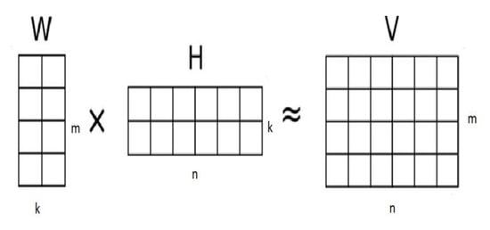
Figure 6. NMF matrix transformations where the dimensions: n and m are determined by the shape of $\mathbf{V}$ and k is determined by the number of components set by the user.

We use nonnegative matrices $\mathbf{W}$ and $\mathbf{H}$, of rank k from which $\mathbf{V}$ is approximated by the dot product operator. Here, k is a parameter set that is usually smaller than the number of rows and columns of $\mathbf{V}$. The trade-off with k is a fine balance, being able to capture the key features of the data but also to avoid overfitting. In our previous work we modified NMF as a data integration method [82]. Other variations are typically used for data integration with heterogeneous data, especially in chemistry and community detection [83,84].

5. Results

The flow of data and processing the posts begins with the conversion of raw text from Twitter, Reddit, and Youtube into Corpora, essentially creating term-document-matrices (as described in Algorithm 1). Once they are processed, we can extract topic models from the Corpora to aid our understanding of the posts due to this logical grouping of keywords.

For an example of sentiment analysis using the R package sentimentr on Twitter posts, see Figure 7. The posts are identified by a number (1–10). They are ranked as either positive (green), neutral (gray), or negative (red), and each has a number denoting the strength of the sentiment. There are three word sentiment lookups available for the Bing, NRC, and Afinn dictionaries, and each has a differing number of words rated and differing sentiment values attached to each word. This can be at the word level, sentence level, or the entire post (paragraph). As can be seen, the Twitter data shown here represents a number of opinions on the climate change debate.

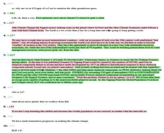
Figure 7. Basic sentiment mining using Twitter data on 10 raw text posts.

We can see that comment 1 is rated at zero sentiment since the sentence is fairly neutral in its wording. In comment 2 we can observe that the first sentence is neutral but the second sentence has a positive sentiment word (optimistic) and is rated +0.082. Comment 3 is more negative because of the words scam, scammer and hoax, rated at −147.

The next stage is to develop topic models holding keywords that are coherently related to key concepts and will be data mined for bigrams. The optimum number of topic models for each Corpora is determined using the Harmonic mean, which is described in Equation (5). In Figure 8, the optimum numbers are presented with 24 for Twitter, 44 for Reddit, and 31 for YouTube concepts and issues. We used LDA to generate the topic maps with a value starting at 10 up to 100 possible topic maps. Therefore, at the first iteration, 10 topic maps would be selected to describe the Corpora, then 11, 12, 13, etc., until 100 topic maps have been generated. Adding more topic maps beyond a certain point would simply degrade the performance. When the harmonic mean decreases, that is the number of maps to use. The harmonic mean method has some known instabilities, but it is in general sufficiently robust.

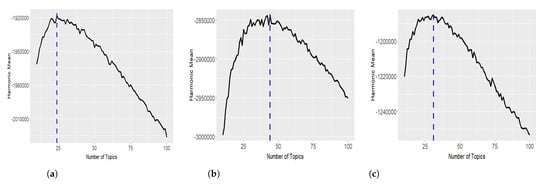
Figure 8. Optimum topic map configuration selected from a range between 10 and 100. (a) Twitter posts generating 24 topic maps. (b) Reddit posts generating 44 topic maps. (c) Youtube posts generating 31 topic maps.

In Figure 9, 5 out of 24 Twitter topic maps are shown. Generally, the terms climate and change are present throughout some of the 24 topic maps. Topic map 2 is generally related to the energy consumption of fossil fuels such as oil and gas. Topic map 3 is concerned with public health and net zero. Topic map 4 has gathered words on environmental impact and statements issued by the Intergovernmental Panel on Climate Change (IPCC). Topic map 5 seems to have grouped human rights and social justice as key themes.

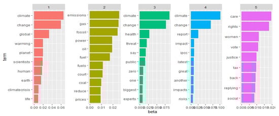
Figure 9. The first five topic maps for Twitter.

To augment the statistics and text mining, we also generated wordclouds, which perhaps give a better visualization and understanding of the main themes that dominate user posts. Individual word frequencies are used to highlight the important themes. The more frequent a word is, the more its size increases. In Figure 10 the wordclouds for Twitter, Reddit, and Youtube are presented. Clearly, climate and change totally dominate the user posts for Twitter, while Reddit and Youtube have a wider range of concepts with more or less equal frequency of occurrence. Only words that appear with at least five occurrences are displayed.

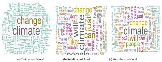
Figure 10. Wordclouds for the posts.

The next stage is to build graph theoretic models of bigrams of co-occurring words building of up a picture of sentiment relating to each Youtube video. The graph models of Twitter and Reddit are also constructed to support the ratings/rankings of the videos in terms of the esteem/trust in which the video producers are held. In Table 3 the graph statistics for YouTube are shown for five users. The key variables are Betweenness and Hubness, which indicates for each word the relative connectivity importance. The other columns have identical values: the mod (modularity) column refers to the structure of the graph and can take a range from 0.0 to 1.0, indicating that there is structure and not a random collection of connections between the nodes. Nedges indicates the number of connections in this small network, nverts is the number of nodes in the network. The transit column refers to the transitivity or community strength. It is a probability for the network to have interconnected adjacent nodes.

Table 3. Graph theoretic statistics of the YouTube bigraph/bigrams of five users.

User	Mod	Path	Nedges	Nverts	Transit	Degree	Diam	Connect	Close	Between	Density	Hubness
UC9Di-3Y41sreUEtKD9MuZEQ	0.69	1.06	128.00	109	0.00	2.35	2.00	FALSE	0.30	19.00	0.01	0.00
UCjjVjhAEzLNAvpr-7pDpd8g	0.69	1.06	128.00	109	0.00	2.35	2.00	FALSE	0.20	15.00	0.01	0.00
UCrsD7Oq3yjZu0GYLhquHpVQ	0.69	1.06	128.00	109	0.00	2.35	2.00	FALSE	0.20	14.00	0.01	0.00
UCUB6baFW4kvLsLzlZ-kp5Ug	0.69	1.06	128.00	109	0.00	2.35	2.00	FALSE	0.50	5.00	0.01	0.00
UCjrCf7x7Dgo4VKplUgWKIdg	0.69	1.06	128.00	109	0.00	2.35	2.00	FALSE	0.50	5.00	0.01	0.00

As the graph is highly disconnected (bigrams linking to other bigrams), it shows zero for all entries. Degree refers to the average number of connection per node, which is is around 2.0, diam is the length of the shortest path between the most distanced nodes. Connect refers to the full connectedness of the graph, which it is not, in this case. Closeness of a node measures its average distance to all other nodes, and a high closeness score suggests a short distances to all other nodes. Betweenness detects the influence a given node has over the flow of information in a graph. The Density represents the ratio between the edges present in a graph and the maximum number of edges that the graph can contain. The Hubness is a value used to indicate the nodes with a larger number of connections than an average node.

Table 4 shows the basic statistics of several YouTube videos. We collected data such as the ID of the video, e.g., in the first row, oJAbATJCugs would normally be used to select the video in a web browser by using the string https://www.youtube.com/watch?v=oJAbATJCugs (accessed on 29 May 2023). The number of comments received for each video is collected, along with the average number of likes. We also collect the number of comments that had zero likes and we should note that this does not imply that the video was disliked, only that the person sending the comment neglected to select like irrespective of their feelings for the video. The number of unique posters posting comments is also recorded. Next we perform sentiment analysis, examining the overall sentiment for the video and then breaking down the comments into neutral, negative, and positive sentiments. The total number of sentiments (positive, negative, and neutral) are based on the sentence level and we therefore have more than the overall number of comments, i.e., the number of posts.

Table 4. Main statistics of the selected YouTube videos.

	vid_id	title	num_comments	likes	zero_likes	num_posters	overall_sentiment	neg_sent_count	pos_sent_count	neut_sent_count
1	oJAbATJCugs	VID1	500	3311	412	57	7.81	501	581	437
2	n-Z0eG1pKhA	VID2	602	1947	364	525	-5.64	528	514	427
3	vFDnknU0h0s	VID3	628	219	536	477	16.88	912	999	669
4	2CQvBGSiDvw	VID4	1114	3399	789	587	0.7	1038	1103	1004
5	ga-RBuhcJ7w	VID5	689	158	627	468	-15.71	911	873	756
6	eDWq7-eP5sE	VID6	680	1185	428	481	30.13	943	1085	714
7	DticpNH3a2Q	VID7	587	72	536	458	-90.32	642	457	371
8	rwdxffEzQ9I	VID8	708	877	561	502	63.59	549	701	565
9	uynhvHZUOOo	VID9	769	300	616	520	-17.37	636	674	651
10	dcBXmj1nMTQ	VID10	625	155	529	488	45.01	594	732	502
11	tMwFNMfjFuU	VID11	98	1289	3	95	14	40	76	43
12	48zAWYkrBIw	VID12	305	1238	162	201	-9.6	288	259	252
13	eDWq7-eP5sE	VID13	679	1185	427	481	29.54	942	1082	713
14	DYWrehjaMFQ	VID14	737	303	585	424	33.96	860	964	565
15	I2OHAuvoUkQ	VID15	374	575	269	196	10.42	367	411	314
16	rweblFwt-BM	VID16	731	1103	512	522	35.25	750	881	659
17	pl1Rnz4zNkg	VID17	628	772	446	534	-35.53	515	454	362
18	qXLqoFHGmv0	VID18	763	1283	503	335	-17.99	811	740	708
19	m3hHi4sylxE	VID19	653	155	536	481	-48.9	773	710	760

The YouTube bigrams are displayed in Figure 11. We only show the words that have at least 100 co-occurrences based on key topic map groupings. The bigrams for YouTube are more strongly linked to coherent topics and follow a logical pattern of subjects with more linkages between bigrams. Generally, the comments on YouTube are more calm and balanced with some thought given to the subject of global warming.

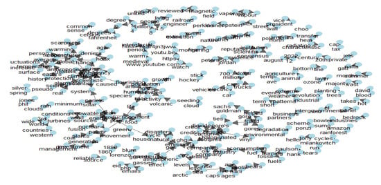
Figure 11. Bigram chart of the YouTube linked pairs of words.

In Figure 12, it can be seen that the situation for Twitter bigrams is more complicated. Additionally, because of the large number of posts, we filter the number of word co-occurrences to 200 before they can appear on the plot. However, it provides a richer source of data by illuminating the issues and concerns once the most frequently occurring words are revealed based on key topic map groupings. The general trend for Twitter posts seems to contain a lot of off-topic issues such as legal aspects and gun violence. Another issue is the text limits on Tweets (280 characters), which may cause posters some constraints in their dialog. The text limit has been raised for fee paying subscribers to 4000 characters.

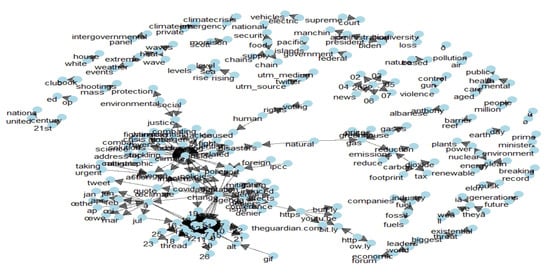
Figure 12. Bigram chart of Twitter linked pairs of words.

In Figure 13 the Reddit bigrams are displayed. Again, for clarity, we only show those words that have at least 100 co-occurrences based on key topic map groupings. Similar in tone and style to YouTube posts, the majority of Reddit posts are more objective and less inclined to be sensationalist. Reddit has very strict rules on posting and any user breaching these may be banned. Other inducements for good behavior are karma awards and coins, which are given to a poster by other users.

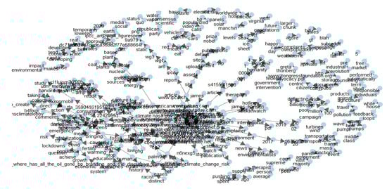
Figure 13. Bigram chart of the Reddit linked pairs of words.

Having gathered statistics from sentiment analysis of the topic maps, comments, and bigrams of paired common words, we now structure the data to build the recommendation engine. The difficulty we face is that the matrix of items (videos) and users is very sparse. This is alleviated to a certain extent by generic profiling of users from Twitter and Reddit data.

The rating matrix is formed from the YouTube user rankings of videos. These are normalized by centering to remove possible rating bias by subtracting the row mean from all ratings in the row. In Table 5 we present normalized ratings data for a small fraction of the overall ratings matrix. Empty spaces represent missing values where no rating data exists. The missing values are usually identified in our software as Not Available (NA). We did not attempt to impute the missing values.

Table 5. Normalized ratings of YouTube videos for 5 users with up to 18 videos—with missing values.

	vid1	vid2	vid3	vid4	vid5	vid6	vid7	vid8	vid9	vid10	vid11	vid12	vid13	vid14	vid15	vid16	vid17	vid18
usr1	−0.24	1.18	0.88	−1.17	0.88	0.06	−0.89	0.25	−0.88	−1.34	−0.52	1.67	0.55	1.36	−1.75	−0.21	0.79	0.72
usr2		0.49	−1.38	−0.22	−0.63	−1.34	1.12	0.55	0.00	−1.34	−0.52	0.06	0.18	0.49	1.17	−0.84	−1.06
usr3	0.30	−0.56	0.59	−1.17	−0.25		−1.18	−0.34	0.44	0.94	−1.15	0.06	−1.65	−0.97	−0.08	−1.16
usr4	−0.50	0.49	0.59	−0.22	−1.01	1.47	0.83	−2.11	−0.88	0.62	1.67	−0.90	0.55	−0.10	0.33	0.42	−0.79	−0.92
usr5	1.63	−1.25	0.88	−0.54		0.34	−0.03		−1.77	−0.04	1.35	1.35	−1.28		−0.92	1.37	1.06	−0.92

In Table 6 we present the model error for the test data. We evaluate the predictions used to compute the deviation of the prediction from the true value. This is the Mean Average Error (MAE). We also use the Root Mean Square Error (RMSE) since it penalizes larger errors than MAE and is thus suitable for situations where smaller errors are likely to be encountered. Here, UBCF is user-based collaborative filtering and IBCF refers to item-based collaborative filtering. We also use mean squared error (MSE) as a measure.

Table 6. Recommender model error on test data.

	RMSE	MSE	MAE
UBCF	5.860	34.344	5.279
IBCF	6.216	38.637	5.573

In Table 7 we display the confusion matrix, where n is the number of recommendations per list, TP, FP, FN, and TN are the entries for true positives, false positives, false negatives, and true negatives. The remaining columns contain precomputed performance measures. We calculate the average for all runs from four-fold cross validation.

Table 7. Confusion matrix for the recommender model indicating averaged error rates (four-fold cross validation).

	TP	FP	FN	TN	N	Precision	Recall	TPR	FPR	n
1	1.00	0.00	10.80	5.20	17.00	1.00	0.09	0.09	0.00	1.00
2	2.20	0.80	9.60	4.40	17.00	0.73	0.18	0.18	0.15	3.00
3	3.40	1.60	8.40	3.60	17.00	0.68	0.28	0.28	0.29	5.00
4	7.20	2.80	4.60	2.40	17.00	0.72	0.61	0.61	0.52	10.00
5	10.80	4.20	1.00	1.00	17.00	0.72	0.91	0.91	0.80	15.00
6	11.80	5.20	0.00	0.00	17.00	0.69	1.00	1.00	1.00	20.00

Examining the evaluation of popular items and the user-based CF methods appear to have a better accuracy and performance than the other methods. In Figure 14, we see that they provide better recommendations than the other method since for each length of top predictions list they have superior values of TPR and FPR. Thus, we have validated our model and are reasonably certain of its robustness.

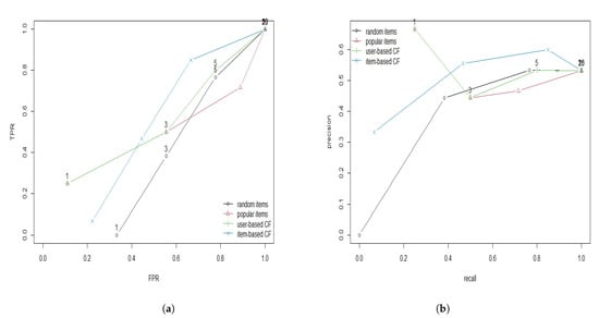
Figure 14. Evaluation of the recommender methods. (a) Comparison of ROC curves for several recommender methods. (b) Comparison of PR curves for several recommender methods.

When in operation, the recommender system makes suggestions for selected users of YouTube based on their ratings of previous videos, their comments (if applicable), and related statistics. In Table 8 we highlight 20 suggestions based on 5 users selected at random. Each user may obtain a differing number of recommendations. Column one identifies the video, column two gives the user ID (selected at random), column three gives the YouTube video ID (which can be pasted into a browser), column four gives the title of the video, column five gives the number of views, and, finally, column six gives the recommender score. Where the videos stand in relation to climate change is obvious from the titles, with the exception of video 20, which appears to take a neutral stance. The score or ranking of a video is based on a value between 0.0 and 1.0, formed by the statistics generated and YouTube recommendations. Experimentally we have determined that values below 0.5 are unlikely to be of interest as we detected videos that are off-topic and minimally related to global warming.

Table 8. Recommendations for five users selected at random.

ID	User	Youtube ID	Video Title	Views	Score
1	1	$cl4Uv{9}_{7}KJE$	Fleeing climate change—the real environmental disaster	2M	1.0
2	1	$K9MaGf-Su9I$	Climate change: Europe’s melting glaciers | DW Documentary	5.7M	1.0
3	1	$3C{M}_{K}kDuzGQ$	Friendly Guide to Climate Change—and what you can do to help	319K	1.0
4	1	$2bXn2F58OsM$	This tool will help us get to zero emissions (Bill Gates)	4.5M	1.0
5	2	$uynhvHZUOOo$	See what three degrees of global warming looks like	3M	1.0
6	2	$zrM1mcKm{X}_c$	Why NITIN GADKARI is pushing GREEN HYDROGEN	2.4M	1.0
7	2	$06m5d3mczvE$	Bill Gates Talks About How To Avoid A Climate Disaster	1.4M	1.0
8	2	$SI9GxjJwGqo$	How long before all the ice melts?—BBC World Service	89K	1.0
9	3	$rwdxffEzQ9I$	El Niño 2023 could be a monster!	1.2M	1.0
10	3	$GystZIxWQ3o$	The melting ice of the Arctic (1/2) | DW Documentary	2.5M	1.0
11	4	$Zklo4Z1SqkE$	Hydrogen Will Not Save Us. Here’s Why.	1.6M	1.0
12	4	$N-yALPEpV4w$	Why renewables can’t save the planet | Michael Shellenberger | TED	5.2M	1.0
13	4	$dPfIU27RGow$	SCIENTISTS JUST MADE HYDROGEN OUT OF NOTHING BUT AIR!!!	104K	1.0
14	4	$yqgMECkW3Ak$	Donald Trump Believes Climate Change Is A Hoax | MSNBC	307K	1.0
15	5	$pwvVephTIHU$	Global warming: why you should not worry	773K	1.0
16	5	$m3hHi4sylxE$	The Truth About Climate Change	2.1M	1.0
17	5	$Qdg4uQW8Dlg$	There is no climate crisis: Tom Harris	1M	1.0
18	5	$YBdmppcfixM$	“There’s no emergency”—dissident climatologist Dr Judith Curry	657K	0.9
19	5	$9Q2YHGIlUDk$	The Models Are OK, the Predictions Are Wrong	876K	0.9
20	5	$1zrejG-WI3U$	Global Warming: Fact or Fiction? Featuring Physicists Soon and Bloom	1M	0.9

6. Conclusions and Future Work

In this paper, we constructed a recommendation system based on sentiment analysis on topic maps, bigrams, and graph analysis. The main source of data was from the posts, comments, and rating statistics attached to each YouTube video. From this data we were able to profile those agreeing with the situation of global warming and those who were more skeptical. Although our model is successful in certain conditions, it has major limitations. Mainly, we cannot usually identify posters from one forum to another. Posters typically have different user-names and so we would most likely not be able to extract further information. Hence, we went for a generic person profiling. We tried to alleviate that drawback by attempting to judge the character, sentiment, and beliefs of the users. Future work must deal with improving user profiling based on their sentiment, type of language they use, and thus gather their opinions and beliefs. Furthermore, it would be interesting to see if some users (tracked over time) change their beliefs. Another interesting possibility would be to suggest videos that conflict with the user’s initial beliefs, assuming that the user is open to persuasion and debate.

References

- Spiliotopoulos, D.; Margaris, D.; Vassilakis, C. On Exploiting Rating Prediction Accuracy Features in Dense Collaborative Filtering Datasets. Information 2022, 13, 428. [Google Scholar] [CrossRef]
- Bai, Y.; Li, Y.; Wang, L. A Joint Summarization and Pre-Trained Model for Review-Based Recommendation. Information 2021, 12, 223. [Google Scholar] [CrossRef]
- Kaur, P.; Goel, S. Shilling attack models in recommender system. In Proceedings of the 2016 International Conference on Inventive Computation Technologies (ICICT), Coimbatore, India, 26–27 August 2016; Volume 2, pp. 1–5. [Google Scholar] [CrossRef]
- Lam, S.K.; Riedl, J. Shilling Recommender Systems for Fun and Profit. In Proceedings of the Proceedings of the 13th International Conference on World Wide Web, New York, NY, USA, 17–20 May 2004; Association for Computing Machinery: New York, NY, USA, 2004; pp. 393–402. [Google Scholar] [CrossRef]
- Sharma, R.; Gopalani, D.; Meena, Y. An anatomization of research paper recommender system: Overview, approaches and challenges. Eng. Appl. Artif. Intell. 2023, 118, 105641. [Google Scholar] [CrossRef]
- Halim, Z.; Hussain, S.; Hashim Ali, R. Identifying content unaware features influencing popularity of videos on YouTube: A study based on seven regions. Expert Syst. Appl. 2022, 206, 117836. [Google Scholar] [CrossRef]
- Zappin, A.; Malik, H.; Shakshuki, E.M.; Dampier, D.A. YouTube Monetization and Censorship by Proxy: A Machine Learning Prospective. Procedia Comput. Sci. 2022, 198, 23–32. [Google Scholar] [CrossRef]
- Grün, B.; Hornik, K. Topicmodels: An R Package for Fitting Topic Models. J. Stat. Softw. 2011, 40, 1–30. [Google Scholar] [CrossRef]
- Smith, B.; Linden, G. Two Decades of Recommender Systems at Amazon.com. IEEE Internet Comput. 2017, 21, 12–18. [Google Scholar] [CrossRef]
- Covington, P.; Adams, J.; Sargin, E. Deep Neural Networks for YouTube Recommendations. In Proceedings of the Proceedings of the 10th ACM Conference on Recommender Systems, Boston, MA, USA, 15–19 September 2016; Association for Computing Machinery: New York, NY, USA, 2016; pp. 191–198. [Google Scholar] [CrossRef]
- Abul-Fottouh, D.; Song, M.Y.; Gruzd, A. Examining algorithmic biases in YouTube’s recommendations of vaccine videos. Int. J. Med. Inform. 2020, 140, 104175. [Google Scholar] [CrossRef]
- Chung, C.Y.; Hsu, P.Y.; Huang, S.H. βP: A novel approach to filter out malicious rating profiles from recommender systems. Decis. Support Syst. 2013, 55, 314–325. [Google Scholar] [CrossRef]
- Kim, Y.; Shim, K. TWILITE: A recommendation system for Twitter using a probabilistic model based on latent Dirichlet allocation. Inf. Syst. 2014, 42, 59–77. [Google Scholar] [CrossRef]
- Abolghasemi, R.; Engelstad, P.; Herrera-Viedma, E.; Yazidi, A. A personality-aware group recommendation system based on pairwise preferences. Inf. Sci. 2022, 595, 1–17. [Google Scholar] [CrossRef]
- Leng, Y.; Yu, L.; Niu, X. Dynamically aggregating individuals’ social influence and interest evolution for group recommendations. Inf. Sci. 2022, 614, 223–239. [Google Scholar] [CrossRef]
- Wu, B.; Ye, Y. BSPR: Basket-sensitive personalized ranking for product recommendation. Inf. Sci. 2020, 541, 185–206. [Google Scholar] [CrossRef]
- Wang, R.; Zhou, D.; Jiang, M.; Si, J.; Yang, Y. A Survey on Opinion Mining: From Stance to Product Aspect. IEEE Access 2019, 7, 41101–41124. [Google Scholar] [CrossRef]
- Singh, N.; Tomar, D.; Sangaiah, A. Sentiment analysis: A review and comparative analysis over social media. J. Ambient. Intell. Humaniz. Comput. 2020, 11, 97–117. [Google Scholar] [CrossRef]
- Birjali, M.; Kasri, M.; Beni-Hssane, A. A comprehensive survey on sentiment analysis: Approaches, challenges and trends. Knowl.-Based Syst. 2021, 226, 107134. [Google Scholar] [CrossRef]
- Phand, S.A.; Phand, J.A. Twitter sentiment classification using stanford NLP. In Proceedings of the 2017 1st International Conference on Intelligent Systems and Information Management (ICISIM), Aurangabad, India, 5–6 October 2017; pp. 1–5. [Google Scholar] [CrossRef]
- Kim, R.Y. Using Online Reviews for Customer Sentiment Analysis. IEEE Eng. Manag. Rev. 2021, 49, 162–168. [Google Scholar] [CrossRef]
- Taboada, M.; Brooke, J.; Tofiloski, M.; Voll, K.; Stede, M. Lexicon-Based Methods for Sentiment Analysis. Comput. Linguist. 2011, 37, 267–307. [Google Scholar] [CrossRef]
- Ding, Y.; Li, B.; Zhao, Y.; Cheng, C. Scoring tourist attractions based on sentiment lexicon. In Proceedings of the 2017 IEEE 2nd Advanced Information Technology, Electronic and Automation Control Conference (IAEAC), Chongqing, China, 25–26 March 2017; pp. 1990–1993. [Google Scholar] [CrossRef]
- Mishev, K.; Gjorgjevikj, A.; Vodenska, I.; Chitkushev, L.T.; Trajanov, D. Evaluation of Sentiment Analysis in Finance: From Lexicons to Transformers. IEEE Access 2020, 8, 131662–131682. [Google Scholar] [CrossRef]
- Crone, S.F.; Koeppel, C. Predicting exchange rates with sentiment indicators: An empirical evaluation using text mining and multilayer perceptrons. In Proceedings of the 2014 IEEE Conference on Computational Intelligence for Financial Engineering and Economics (CIFEr), London, UK, 27–28 March 2014; pp. 114–121. [Google Scholar] [CrossRef]
- Romero, C.; Ventura, S. Educational data mining: A review of the state of the art. IEEE Trans. Syst. Man Cybern. Part C Appl. Rev. 2010, 40, 601–618. [Google Scholar] [CrossRef]
- Kumar, A.; Jai, R. Sentiment analysis and feedback evaluation. In Proceedings of the in 2015 IEEE 3rd International Conference on MOOCs, Innovation and Technology in Education (MITE), Amritsar, India, 1–2 October 2015; pp. 433–436. [Google Scholar]
- Missikoff, M.; Velardi, P.; Fabriani, P. Text mining techniques to automatically enrich a domain ontology. Appl. Intell. 2003, 18, 323–340. [Google Scholar] [CrossRef]
- McGarry, K.; McDonald, S. Computational methods for text mining user posts on a popular gaming forum for identifying user experience issues. In Proceedings of the The 2017 British Human Computer Interaction Conference—Make Believe, Sunderland, UK, 3–6 July 2017. [Google Scholar] [CrossRef]
- Bose, S. RSentiment: A Tool to Extract Meaningful Insights from Textual Reviews. In Proceedings of the 5th International Conference on Frontiers in Intelligent Computing: Theory and Applications: FICTA 2016; Springer: Singapore, 2017; Volume 2, pp. 259–268. [Google Scholar] [CrossRef]
- Seetharamulu, B.; Reddy, B.N.K.; Naidu, K.B. Deep Learning for Sentiment Analysis Based on Customer Reviews. In Proceedings of the 2020 11th International Conference on Computing, Communication and Networking Technologies (ICCCNT), Kharagpur, India, 1–3 July 2020; pp. 1–5. [Google Scholar] [CrossRef]
- Thakur, N. Sentiment Analysis and Text Analysis of the Public Discourse on Twitter about COVID-19 and MPox. Big Data Cogn. Comput. 2023, 7, 116. [Google Scholar] [CrossRef]
- Fellnhofer, K. Positivity and higher alertness levels facilitate discovery: Longitudinal sentiment analysis of emotions on Twitter. Technovation 2023, 122, 102666. [Google Scholar] [CrossRef]
- Di Cara, N.H.; Maggio, V.; Davis, O.S.P.; Haworth, C.M.A. Methodologies for Monitoring Mental Health on Twitter: Systematic Review. J. Med. Internet Res. 2023, 25, e42734. [Google Scholar] [CrossRef]
- Kavitha, K.; Shetty, A.; Abreo, B.; D’Souza, A.; Kondana, A. Analysis and Classification of User Comments on YouTube Videos. Procedia Comput. Sci. 2020, 177, 593–598. [Google Scholar] [CrossRef]
- Alhabash, S.; Jong Hwan, B.; Cunningham, C.; Hagerstrom, A. To comment or not to comment?: How virality, arousal level, and commenting behavior on YouTube videos affect civic behavioral intentions. Comput. Hum. Behav. 2015, 51, 520–531. [Google Scholar] [CrossRef]
- Shiryaeva, T.A.; Arakelova, A.A.; Tikhonova, E.V.; Mekeko, N.M. Anti-, Non-, and Dis-: The linguistics of negative meanings about youtube. Heliyon 2020, 6, e05763. [Google Scholar] [CrossRef]
- Albert, R.; Barabasi, A. Statistical mechanics of complex networks. Rev. Mod. Phys. 2002, 74, 450–461. [Google Scholar] [CrossRef]
- Barabasi, A. Network Science, 1st ed.; Cambridge University Press: Cambridge, UK, 2016. [Google Scholar]
- McGarry, K.; McDonald, S. Complex network theory for the identification and assessment of candidate protein targets. Comput. Biol. Med. 2018, 97, 113–123. [Google Scholar] [CrossRef]
- Ward, K. Social networks, the 2016 US presidential election, and Kantian ethics: Applying the categorical imperative to Cambridge Analytica’s behavioral microtargeting. J. Media Ethics 2018, 33, 133–148. [Google Scholar] [CrossRef]
- Kolaczyk, E. Statistical Research in Networks - Looking Forward. In Encyclopedia of Social Network Analysis and Mining; Springer: New York, NY, USA, 2014; pp. 2056–2062. [Google Scholar] [CrossRef]
- Cai, H.; Zhang, F. Detecting shilling attacks in recommender systems based on analysis of user rating behavior. Knowl.-Based Syst. 2019, 177, 22–43. [Google Scholar] [CrossRef]
- Cruickshank, I.; Carley, K. Characterizing communities of hashtag usage on twitter during the 2020 COVID-19 pandemic by multi-view clustering. Appl. Netw. Sci. 2020, 5, 66. [Google Scholar] [CrossRef]
- Ahmad, U.; Zahid, A.; Shoaib, M.; AlAmri, A. HarVis: An integrated social media content analysis framework for YouTube platform. Inf. Syst. 2017, 69, 25–39. [Google Scholar] [CrossRef]
- Wang, S.; Zhang, P.; Wang, H.; Yu, H.; Zhang, F. Detecting shilling groups in online recommender systems based on graph convolutional network. Inf. Process. Manag. 2022, 59, 103031. [Google Scholar] [CrossRef]
- Keramatfar, A.; Amirkhani, H.; Bidgoly, A.J. Multi-thread hierarchical deep model for context-aware sentiment analysis. J. Inf. Sci. 2023, 49, 133–144. [Google Scholar] [CrossRef]
- Keramatfar, A.; Rafaee, M.; Amirkhani, H. Graph Neural Networks: A bibliometrics overview. Mach. Learn. Appl. 2022, 10, 100401. [Google Scholar] [CrossRef]
- Nilashi, M.; Ali Abumalloh, R.; Samad, S.; Minaei-Bidgoli, B.; Hang Thi, H.; Alghamdi, O.; Yousoof Ismail, M.; Ahmadi, H. The impact of multi-criteria ratings in social networking sites on the performance of online recommendation agents. Telemat. Inform. 2023, 76, 101919. [Google Scholar] [CrossRef]
- Heidari, M.; Jones, J.H.J.; Uzuner, O. An Empirical Study of Machine learning Algorithms for Social Media Bot Detection. In Proceedings of the 2021 IEEE International IOT, Electronics and Mechatronics Conference (IEMTRONICS), Toronto, ON, Canada, 21–24 April 2021; pp. 1–5. [Google Scholar] [CrossRef]
- Heidari, M.; Jones, J.H.; Uzuner, O. Deep Contextualized Word Embedding for Text-based Online User Profiling to Detect Social Bots on Twitter. In Proceedings of the 2020 International Conference on Data Mining Workshops (ICDMW), Sorrento, Italy, 17–20 November 2020; pp. 480–487. [Google Scholar] [CrossRef]
- K, H.; S, S.; M, M. Social media bot detection with deep learning methods: A systematic review. Neural Comput. Appl. 2023, 35, 8903–8918. [Google Scholar] [CrossRef]
- Schneider, L.; Scholten, J.; Sándor, B. Charting closed-loop collective cultural decisions: From book best sellers and music downloads to Twitter hashtags and Reddit comments. Eur. Phys. J. B 2021, 94. [Google Scholar] [CrossRef]
- Madsen, M.A.; Madsen, D.O. Communication between Parents and Teachers of Special Education Students: A Small Exploratory Study of Reddit Posts. Soc. Sci. 2022, 11, 518. [Google Scholar] [CrossRef]
- Harel, T.L. Archives in the making: Documenting the January 6 capitol riot on Reddit. Internet Hist. 2022, 6, 391–411. [Google Scholar] [CrossRef]
- SemRush-Inc. Reddit Statistics. Available online: https://www.semrush.com/website/reddit.com/overview/, (accessed on 4 February 2023).
- Chew, R.F.; Kery, C.; Baum, L.; Bukowski, T.; Kim, A.; Navarro, M.A. Predicting Age Groups of Reddit Users Based on Posting Behavior and Metadata: Classification Model Development and Validation. JMIR Public Health Surveill. 2021, 7, e25807. [Google Scholar] [CrossRef]
- Barker, J.; Rohde, J. Topic Clustering of E-Cigarette Submissions Among Reddit Communities: A Network Perspective. Health Educ. Behav. 2019, 46. [Google Scholar] [CrossRef] [PubMed]
- Gaffney, D.; Matias, J. Caveat emptor, computational social science: Large-scale missing data in a widely-published Reddit corpus. PLoS ONE 2018, 13, e0200162. [Google Scholar] [CrossRef] [PubMed]
- Jhaver, S.; Appling, D.S.; Gilbert, E.; Bruckman, A. “Did You Suspect the Post Would Be Removed?”: Understanding User Reactions to Content Removals on Reddit. Proc. ACM Hum.-Comput. Interact. 2019, 3, 1–33. [Google Scholar] [CrossRef]
- Baumgartner, J.; Zannettou, S.; Keegan, B.; Squire, M.; Blackburn, J. The Pushshift Reddit Dataset. Proc. Int. AAAI Conf. Web Soc. Media 2020, 14, 830–839. [Google Scholar] [CrossRef]
- Rivera, I. Reddit Data Extraction Toolkit. 2023. Available online: https://cran.r-project.org/web/packages/RedditExtractoR/index.html (accessed on 29 June 2023).
- Gertzel, B.; Ackland, R.; Graham, T.; Borquez, F. VosonSML: Collecting Social Media Data and Generating Networks for Analysis. 2022. Available online: https://cran.r-project.org/web/packages/vosonSML/index.html (accessed on 29 June 2023).
- Bauchi, C. Twitter Climate Change Sentiment Dataset. 2018. Available online: https://www.kaggle.com/datasets/edqian/twitter-climate-change-sentiment-dataset (accessed on 29 June 2023).
- Rinker, T.W. Sentimentr: Calculate Text Polarity Sentiment; Buffalo, NY, USA. 2021. Available online: github.com/trinker/sentimentr (accessed on 30 May 2023).
- Feinerer, I.; Hornik, K.; Meyer, D. Text Mining Infrastructure in R. J. Stat. Softw. 2008, 25, 1–54. [Google Scholar] [CrossRef]
- Feinerer, I.; Hornik, K. tm: Text Mining Package; R package version 0.7-11; The R Project for Statistical Computing: Vienna, Austria, 2023. Available online: https://CRAN.R-project.org/package=tm (accessed on 30 May 2023).
- Chen, Y.L.; Chang, C.L.; Yeh, C.S. Emotion classification of YouTube videos. Decis. Support Syst. 2017, 101, 40–50. [Google Scholar] [CrossRef]
- Chang, W.L.; Chen, L.M.; Verkholantsev, A. Revisiting Online Video Popularity: A Sentimental Analysis. Cybern. Syst. 2019, 50, 563–577. [Google Scholar] [CrossRef]
- Gandhi, A.; Adhvaryu, K.; Poria, S.; Cambria, E.; Hussain, A. Multimodal sentiment analysis: A systematic review of history, datasets, multimodal fusion methods, applications, challenges and future directions. Inf. Fusion 2023, 91, 424–444. [Google Scholar] [CrossRef]
- Rouhani, S.; Mozaffari, F. Sentiment analysis researches story narrated by topic modeling approach. Soc. Sci. Humanit. Open 2022, 6, 100309. [Google Scholar] [CrossRef]
- Csardi, G.; Nepusz, T. The igraph software package for complex network research. Interjournal Complex Syst. 2006, 1695, 1–9. [Google Scholar]
- Li, J.; Wang, Y.; Tao, Z. A Rating Prediction Recommendation Model Combined with the Optimizing Allocation for Information Granularity of Attributes. Information 2022, 13, 21. [Google Scholar] [CrossRef]
- Blei, D.M.; Ng, A.Y.; Jordan, M.I. Latent dirichlet allocation. J. Mach. Learn. Res. 2003, 3, 993–1022. [Google Scholar]
- Grün, B.; Hornik, K. R Package Topicmodels. Available online: https://cran.r-project.org/web/packages/topicmodels/index.html (accessed on 12 June 2023).
- Chang, J.; Gerrish, S.; Wang, C.; Boyd-graber, J.; Blei, D. Reading Tea Leaves: How Humans Interpret Topic Models. In Proceedings of the Advances in Neural Information Processing Systems; Bengio, Y., Schuurmans, D., Lafferty, J., Williams, C., Culotta, A., Eds.; Curran Associates, Inc.: New York, NY, USA, 2009; Volume 22. [Google Scholar]
- Griffiths, T.; Steyvers, M. Finding scientific topics. Proc. Natl. Acad. Sci. USA 2004, 101, 5228–5235. [Google Scholar] [CrossRef]
- Gaujoux, R.; Seoighe, C. A flexible R package for nonnegative matrix factorization. BMC Bioinform. 2010, 11, 367. [Google Scholar] [CrossRef]
- Greene, D.; Cunningham, P. A Matrix Factorization Approach for Integrating Multiple Data Views. In Proceedings of the Machine Learning and Knowledge Discovery in Databases; Buntine, W., Grobelnik, M., Eds.; Springer: Berlin/Heidelberg, Germany, 2009; pp. 423–438. [Google Scholar]
- Vlachos, M.; Dunner, C.; Heckle, R.; Vassiliadis, A.; Parnell, T.; Atasu, K. Addressing interpretability and cold-start in matrix factorization for recommender systems. IEEE Trans. Knowl. Data Eng. 2019, 31, 1253–1266. [Google Scholar] [CrossRef]
- Hahsler, M. Recommenderlab: An R Framework for Developing and Testing Recommendation Algorithms. arXiv 2022, arXiv:cs.IR/2205.12371. [Google Scholar]
- McGarry, K.; Graham, Y.; McDonald, S.; Rashid, A. RESKO: Repositioning drugs by using side effects and knowledge from ontologies. Knowl. Based Syst. 2018, 160, 34–48. [Google Scholar] [CrossRef]
- Wang, J.; Fan, Z.; Cheng, Y. Drug disease association and drug repositioning predictions in complex diseases using causal inference probabilistic matrix factorization. J. Chem. Inf. Model. 2014, 54, 2562–2569. [Google Scholar]
- Li, W.; Xie, J.; Mo, J. An overlapping network community partition algorithm based on semi-supervised matrix factorization and random walk. Expert Syst. Appl. 2018, 91, 277–285. [Google Scholar] [CrossRef]
Disclaimer/Publisher’s Note: The statements, opinions and data contained in all publications are solely those of the individual author(s) and contributor(s) and not of MDPI and/or the editor(s). MDPI and/or the editor(s) disclaim responsibility for any injury to people or property resulting from any ideas, methods, instructions or products referred to in the content. |
© 2023 by the author. Licensee MDPI, Basel, Switzerland. This article is an open access article distributed under the terms and conditions of the Creative Commons Attribution (CC BY) license (https://creativecommons.org/licenses/by/4.0/).