Innovating Intrusion Detection Classification Analysis for an Imbalanced Data Sample

Abstract

This work is designed to assist researchers and interested learners in comprehending and putting deep machine learning classification approaches into practice. It aimed to simplify, facilitate, and advance classification methodology skills. To make it easier for the users to understand, it employed a methodical approach. The categorization assessment measures seek to give the fundamentals of these measures and demonstrate how they operate to function as a comprehensive resource for academics interested in this area. Intrusion detection and threat analysis (IDAT) is a particularly unpleasant cybersecurity issue. In this study, IDAT is identified as a case study, and a real-sample dataset that was used for institutional and community awareness was generated by the researchers. This review shows that, to solve a classification problem, it is crucial to use the output of classification in terms of performance measurements, encompassing both conventional criteria and contemporary metrics. This study focused on addressing the dynamic of classification assessment capabilities for using both scalars and visual metrics, and to fix imbalanced dataset difficulties. In conclusion, this review is a useful tool for researchers, especially when they are working on big data preprocessing, handling imbalanced data for multiclass assessment, and ML classification.

1. Introduction

Intrusion detection system (IDS) classification methods are in extreme demand to secure institutions against a massive type of cybercrime risks spreading nowadays [1]. IDS warning systems require an early and correct prediction mechanism to save a community against its devastating risks [2,3]. Many effective IDS assessment articles were published; however, institutions have not reached a unified methodology yet [4]. This study aimed to determine an accurate classification metric that can be used to address IDS analysis. In addition, this work was designed to promote community awareness against aggressive IDS threats.

Classifying IDS offers many benefits: (1) it can detect attacks as they occur; (2) it has the ability to use different methodologies for monitoring attacks; (3) it has the flexibility to be installed on either local hosts or networks; and, finally, (4) it can be extended to cover prevention domains.

Researchers have calculated that the ratio of attack samples to total payload traffic for an IDS data mining system can range from 1 to 5% [5]. Standard classifiers for ML learning may bias the majority/normal classifications with high accuracy and low attack detection. The objective of this study is to minimize false alarms and maximize detection of minority attack classes.

IDS has faced numerous difficulties [2,6], including (1) a high false-negative rate, which happens when attacks are mistakenly identified as legitimate traffic and are considered critical failures; (2) class overlapping, which makes categorization challenging and happens when certain attacks mimic regular traffic; (3) idea drift, as network behaviors evolve over time; and (4) scalability, as IDS must function in real time while dealing with high traffic volumes.

Three different solution approaches have been introduced to handle the case of imbalanced datasets [3,7]. Figure 1 offers these imbalanced dataset-manipulating methods, which are elaborated upon in the Section 3.

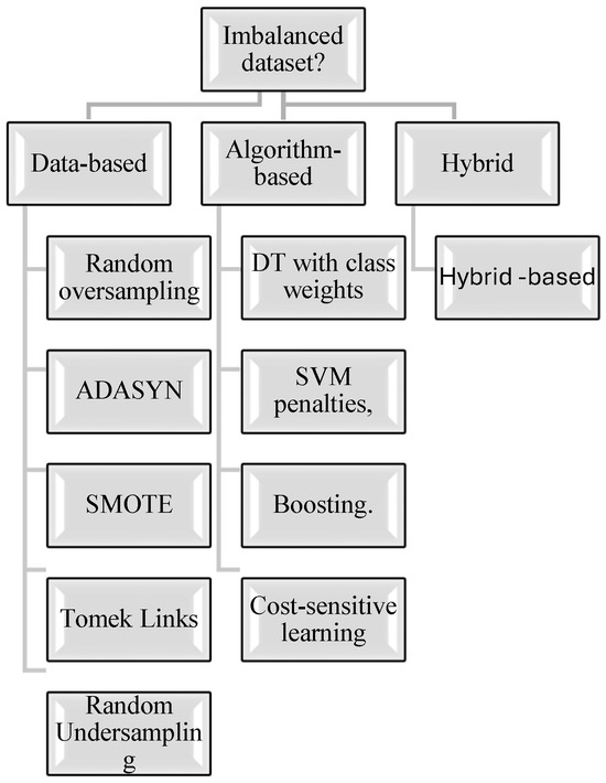
Figure 1. Imbalanced dataset manipulation methods.

Many articles have been published that address IDS imbalance datasets, and although they performed well, they failed to solve the problem of attack majority rates [8,9].

The objectives of this manuscript are to assess classifiers’ competency for the IDS, handle imbalance challenges for multiclass data, and compare some methods. However, this study’s key contributions include, but are not limited to, providing a rich IDS sample dataset capable of researchers’ open use, controlling the imbalance in the multiclass dataset, and examining some powerful insight classifiers’ conclusions. The following research questions were formulated to guide the reviewer/reader and ease the paper’s understandability, as well as its readability.

This paper is designed to serve as a reliable research aid that can be widely used/developed to help researchers analyze and perform critical problems regarding IDS. In this respect, this paper uses a step-by-step mode of processing and considering learnability/educational, rather than using an investigative approach. Figure 2 below illustrates the methodology processes which denote the step-by-step mode of processing.

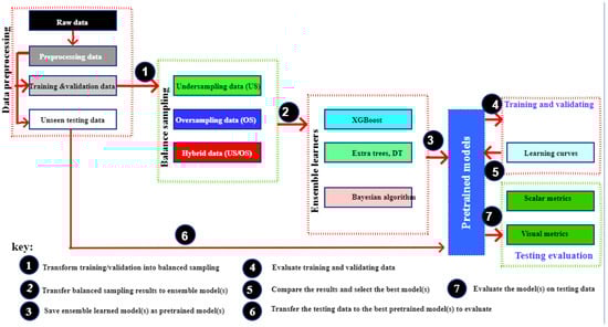
Figure 2. A step-by-step mode of processing.

―

How do IDC assessments direct the classifiers’ analysis domains related to cybersecurity aspects?

―

What kind of output(s) dominates IDS classification exploring the dataset?

―

What implications do these findings have for IDS policy and strategy?

This paper is organized as follows, with a logical flow from the Introduction to the Conclusion section: The literature review and the recently linked articles are covered in Section 2. The materials and methods used are presented in Section 3. Experiments and results are shown in Section 4. Section 5 offers a discussion and concludes the study, and it is followed by the references.

2. Related Works

Intrusion detection for an imbalanced classification dataset defines a case where the distribution of a dataset’s classes in a classification problem is un-binary [1,2]. It happens when the model performs better in the majority class, and vice versa with the minority ones. Cybercrime detection, medical testing, and IDS are among the popular examples of imbalanced datasets. Such minority classification problems create critical cases that may lead to a model’s outperformance being biased and violated [4]. These challenges include, but are not limited to, the following: (1) bias with respect to majority class; (2) poor recall (decrease sensitivity), which occurs when the system fails to classify true cases in the minority class; and (3) decentralization, which means that the model demonstrates low capability in regard to the minority.

Very effective methods can be used to control imbalanced datasets; however, picking a specific one refers to the degree of accuracy and the model’s fitness. These methods are defined as follows:

―

Recruit a sophisticated metric that is capable of clarifying the model’s performance form, particularly with a minority set. Such metrics include recall, precision, F1-score, ROC, and AUC curves.

―

SMOTE, which stands for synthetic minority oversampling technique, is used to perfectly balance/reduce the number of majority sets. It is highly effective; however, it causes data loss.

―

Algorithm-based tuning is used to balance or adapt higher weights for the minority set to minimize bias. It is major sampling method that offers cost-sensitive learning and class-weighted models, and it fixes imbalance influence. Algorithms such as random forest and XGBoost are the most effective ones.

―

Data augmentation is an amazingly effective technique used to augment the minority set by rotating or flipping to balance the dataset.

―

The anomaly technique is an anomaly detection method used to control the minority class.

―

Understandability of the domain is useful, granted that the minority class is rare.

―

Experimental methods are used to examine different resampling methods, models, and measures.

―

CV-based methods use different combinations/permutation to validate the system’s performance to achieve generalization.

Unbalanced datasets are a frequent problem in machine learning, but their effects can be lessened to create strong models that function well in all classes, using the correct methods and assessment criteria [7].

Massive studies have been conducted evaluating IDS with ML tools; nevertheless, the door is open for introducing new methods/algorithms that positively fix the challenges. Reference [8] provides a comprehensive classification evaluation using both scalar and visual measures and adds a general educational value; however, it lacks implementation on a real imbalanced dataset and lacks practical testing performed under a modern performance criterion. This is because it was designed to serve as an analysis reference. Following a step-by-step method, it was successfully demonstrated to assess the impacts of imbalanced datasets across different measurements, particularly plotting ROC-AUC, PR, and DET curves. Its limitations can be summarized as follows: (1) it does not perfectly cover modern classification metrics such as Cohen’s Kappa, macro/micro means for multiclass configurations, and cost-sensitive; (2) it only focuses on traditional methods, with update metrics like calibration curves, Brier scores, or probability methods not being covered; and (3) it is not associated with a domain-specific application field.

As a reference for assessing imbalanced data evaluation problems, Ref. [7] offers a well-designed and comprehensive survey classification method for the domains where a class-imbalanced dataset is critical. It is a theoretical foundation and very significant paper for imbalanced dataset techniques. However, it lacks empirical practice and offers no depth in regard to modern techniques.

Table 1 presents IDS-imbalanced classification articles and assessment-methodology selection and gives the recently published articles on imbalanced dataset assessment strategies, along with their corresponding performance metrics that were implemented to develop imbalanced classification algorithms. It identifies the dates, contributions, and methods/algorithms used, along with their limitations. Table 1 quietly figures out the research gap in this issue and helps to illustrate each study’s contribution.

Table 1. IDS-imbalanced classification articles and assessment-methodology selection.

Approach	Implication	+	−	Domain(s)	Criteria	Review	Article(s), Year	Method	Imbalanced	Metrics Used	Contribution
Data level [10,11]	Random oversampling, SMOTE, ADASYN. Random undersampling Tomek links	Simple, model-agnostic, balances class distribution	Oversampling may cause overfitting. Undersampling may lose useful data	Medical diagnosis, text classification, fraud detection	F1-score, precision–recall curve (PR) curve, G-mean	Suited for PR curves and G-mean, since they directly affect class distributions	[10], 2023	GAN-based	GAN synthetic oversampling	Acc, precision, recall, F1	GANs for minority attack classes
							[11], 2023	Empirical (under/over/hybrid-sampling)	Sampling metric	Precision, recall, F1, AUC	Comprehensive review
Algorithm level [12,13,14,15,16]	Cost-sensitive learning. Decision Trees with class weights, SVM penalties, boosting	Directly modifies algorithms, avoids altering data distribution.	Requires algorithm-specific tuning, may increase computational cost	Intrusion detection, financial risk assessment, cybersecurity	ROC-AUC, MCC, balanced accuracy	Better assessed with ROC-AUC and MCC, as they optimize decision boundaries	[12], 2024	Ensemble ML	limited	Acc, recall, F1	Collaborative IDS across edge systems
							[13], 2024	DL	indirect	Acc, precision, recall, F1	Feature interaction modeling
							[14], 2023	Tree-based ensemble	Algorithm-level imbalance robustness	Acc, recall, F1	Multiclass ensemble IDS
							[15], 2021	ML-based (SVM, RF, KNN)	Nor addressed	Acc, detection rate	Comparative, baseline CAN-bus IDS
							[16], 2021	AdaBoost	Algorithm-level	Acc, AUC, F1	Improved AdaBoost for imbalance
Hybrid [17,18,19]	SMOTE, boosting, ensemble with resampling, GAN-based synthetic data + classifier	Combines strengthens of both approaches, often best performance	More complex to implement, risk of high computational cost	Rare-disease detection, image recognition	ROC-AUAUC, F1-score, MCC	Typically evaluated with a mix (PR-AUC + ROC-AUC + MCC), since they combine both strategies	[17], 2023	Reinforcement learning + sampling	Adaptive over/under sampling	Acc, precision, recall, F1	RL-driven dynamic imbalance handling
							[18], 2024	LSTM, feature selection, SMOTE	SMOTE oversampling	Acc, precision, recall, F1	Merges DL plus resampling
							[19], 2025	ML (RF, XGB, DL)	evaluation	Acc, precision, recall, F1	Top IDS handles multiclass imbalance

There are three main categories of recent research on intrusion detection and classification under unbalanced data: data-level, algorithm-level, and hybrid techniques. Data-level approaches that balance the dataset before model training, such as GAN-based oversampling [10] and empirical studies of resampling techniques [11], provide simplicity and model independence but run the risk of producing artificial noise or overfitting. Although they frequently require intricate tuning and may not work well on highly skewed distributions, algorithm-level approaches such as ensemble frameworks [12,14], deep feature-interaction models [13], and boosting enhancements [16] modify learning algorithms to better handle imbalance. Hybrid approaches, which combine resampling and algorithmic modifications, are becoming increasingly popular. Examples of these include reinforcement learning frameworks with over/undersampling [17] and SMOTE with LSTM-based models [18]. Interestingly, Ref. [10] optimizes machine learning models on unbalanced data, offering one of the first focused investigations of multi-class intrusion detection in the Internet of Vehicles (IoV). The research shows a distinct tendency toward hybrid methods, which provide stronger generalization in actual IDS contexts but come with higher computational and design complexity.

As shown in Table 1, the literature review was separated into three categories: data level [10,11], algorithm level [12,13,14,15,16]), and hybrid [17,18,19]. This classification clarified the gaps, and most of the articles are at the algorithm level, with a few more recent ones being hybrid. The most recent perspective is the Internet of Vehicles (IoV) with multiclass imbalance [19].

3. Materials and Methods

Here, we used an IDS dataset controlled by ML processes to form a powerful environment. These processes varied to include preprocessing steps, resampling examples, and class training of cost-sensitive models, followed by the recruited core classification formulas, evaluation measures, and, finally, the model’s deployment and validation of the concepts and method.

3.1. Overview of the Dataset

The infrastructure networks of actual institutions were used to collect the datasets needed for this study, and the authors attested that the network was constructed and utilized exclusively for research and to protect the local community from malevolent cyberattacks. For the purpose of creating their dataset, the authors at Jazan University used a university network with a Saudi national network backbone. This network provides the dynamic of small/large interconnection lengths at high data speeds.

Preprocessing the dataset is an indispensable step and requires major tasks in data preprocessing to promote its quality. These tasks are data cleaning, integration, reduction, transformation, and discretization. In this section, we summarized how our raw dataset [20] was cleaned by removing the noise, errors, and missing data, and how it was reduced and preprocessed to support IDS classification assessment.

This dataset includes 120 features that describe network traffic and security-log attributes, together with 1,048,575 records. An overview of these properties, including their data formats, counts of unique values, and the quantity of missing (NaN) values, is given in Table 2.

Table 2. Dataset summary.

Column Name	Data Type	Unique Values Count	NaN Count
Domain	int64	1	0
Receive Time	datetime64[ns]	53,466	0
Serial #	int64	1	0
Type	object	1	0
Threat/Content Type	object	7	0
Config Version	int64	1	0
Generate Time	datetime64[ns]	53,466	0
Source Address	object	9744	0
Destination Address	object	6624	0
NAT Source IP	object	10	1,033,000
NAT Destination IP	object	818	1,033,000
Rule	object	17	549,532
Source User	object	4234	391,310
Destination User	object	1421	842,969
Application	object	15	0
Virtual System	object	1	0
Source Zone	object	5	0
Destination Zone	object	6	1
Inbound Interface	object	5	1
Outbound Interface	object	6	549,532
Log Action	object	2	1,037,148
Time-Logged	datetime64[ns]	53,466	0
Session ID	int64	462,478	0
Repeat Count	int64	102	0
Source Port	int64	42,788	0
Destination Port	int64	969	0
NAT Source Port	int64	13,400	0
NAT Destination Port	int64	7	0
Flags	object	11	0
IP Protocol	object	3	0
Action	object	5	0
URL/Filename	object	28	1,048,035
Threat/Content Name	object	43	0
Category	object	13	0
Severity	object	5	0
Direction	object	2	0
Sequence Number	int64	1056	0
Action Flags	object	2	0
Source Country	object	35	0
Destination Country	object	79	0
Unnamed: 40	float64	0	1,048,575
Contenttype	float64	0	1,048,575
pcap_id	int64	1	0
Filedigest	float64	0	1,048,575
Cloud	float64	0	1,048,575
url_idx	int64	9	0
user_agent	float64	0	1,048,575
Filetype	float64	0	1,048,575
Xff	float64	0	1,048,575
Referrer	float64	0	1,048,575
Sender	float64	0	1,048,575
Subject	float64	0	1,048,575
Recipient	float64	0	1,048,575
Reported	int64	1	0
DG Hierarchy Level 1	int64	1	0
DG Hierarchy Level 2	int64	1	0
DG Hierarchy Level 3	int64	1	0
DG Hierarchy Level 4	int64	1	0
Virtual System Name	object	1	0
Device Name	object	1	0
file_url	float64	0	1,048,575
Source VM UUID	float64	0	1,048,575
Destination VM UUID	float64	0	1,048,575
http_method	float64	0	1,048,575
Tunnel ID/IMSI	int64	1	0
Monitor Tag/IMEI	float64	0	1,048,575
Parent Session ID	int64	1	0
Parent Session Start Time	float64	0	1,048,575
Tunnel	float64	0	1,048,575
thr_category	object	11	0
Contentver	object	5	0
sig_flags	object	2	0
SCTP Association ID	int64	1	0
Payload Protocol ID	int64	1	0
http_headers	float64	0	1,048,575
URL Category List	float64	0	1,048,575
UUID for Rule	object	17	549,532
HTTP/2 Connection	int64	1	0
dynusergroup_name	float64	0	1,048,575
XFF Address	float64	0	1,048,575
Source Device Category	float64	0	1,048,575
Source Device Profile	float64	0	1,048,575
Source Device Model	float64	0	1,048,575
Source Device Vendor	float64	0	1,048,575
Source Device OS Family	float64	0	1,048,575
Source Device OS Version	float64	0	1,048,575
Source Hostname	float64	0	1,048,575
Source Mac Address	float64	0	1,048,575
Destination Device Category	float64	0	1,048,575
Destination Device Profile	float64	0	1,048,575
Destination Device Model	float64	0	1,048,575
Destination Device Vendor	float64	0	1,048,575
Destination Device OS Family	float64	0	1,048,575
Destination Device OS Version	float64	0	1,048,575
Destination Hostname	float64	0	1,048,575
Destination Mac Address	float64	0	1,048,575
Container ID	float64	0	1,048,575
POD Namespace	float64	0	1,048,575
POD Name	float64	0	1,048,575
Source External Dynamic List	float64	0	1,048,575
Destination External Dynamic List	float64	0	1,048,575
Host ID	float64	0	1,048,575
Serial Number	float64	0	1,048,575
domain_edl	float64	0	1,048,575
Source Dynamic Address Group	float64	0	1,048,575
Destination Dynamic Address Group	float64	0	1,048,575
partial_hash	int64	1	0
High-Res Timestamp	object	85,581	0
Reason	float64	0	1,048,575
Justification	float64	0	1,048,575
nssai_sst	float64	1	49,9043
Subcategory of App	object	8	0
Category of App	object	6	0
Technology of App	object	4	0
Risk of App	int64	4	0
Characteristics of App	object	9	549,532
Container of App	object	5	752,386
Tunneled App	object	9	0
SaaS of App	object	2	0
Sanctioned State of App	object	1	0

3.2. Preprocessing

For illustrative purposes, this section will use a small randomly selected sample of 100 datapoints from the main dataset. The analysis will focus on 10 features relevant to intrusion detection: “Time-Logged”, “Threat/Content Type”, “Repeat Count”, “Source Zone”, “Source Port”, “Category of App”, “Source Country”, “Type”, “Destination Country”, and “Action”.

3.3. Visualization

Visualization represents a key phase in the exploration of the data ware. Figure 3a–j offer some important feature exploration plots, with a comparison between the entire dataset (left) and 100 randomly selected datapoints (right) used as a primary state to guide a researcher in performing deep learning and mining inside the dataset.

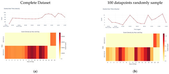
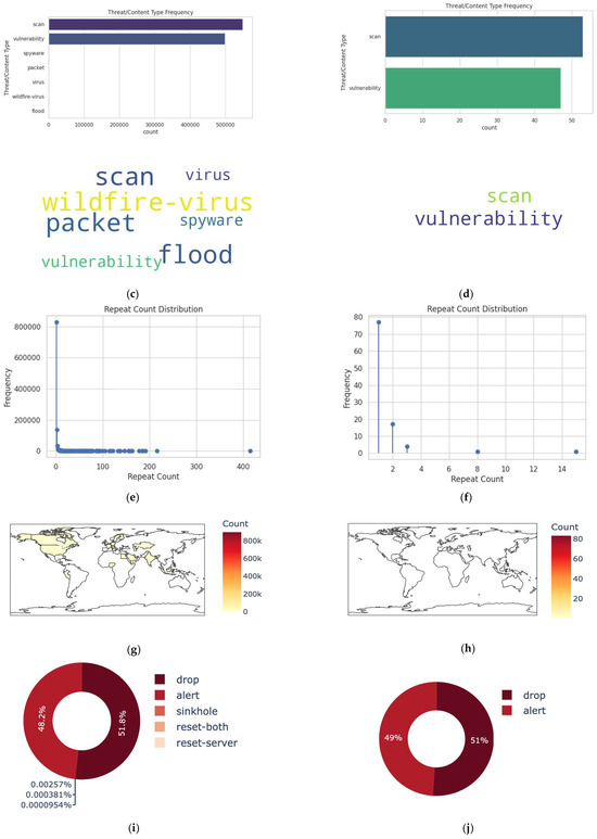
Figure 3. Some important feature exploration plots with comparison between the entire dataset (left) and 100 randomly selected datapoints (right). (a) Data visualization for the whole dataset. (b) Data visualization for 100 datapoints. (c) Data visualization for the whole dataset—Time-Logged. (d) Data visualization for 100 datapoints—Time-Logged. (e) Threat/Content Type for the whole dataset. (f) Threat/Content Type for 100 datapoints. (g) Repeat count type for the whole dataset. (h) Repeat count type for the 100 datapoints. (i) Distribution type for the whole dataset. (j) Distribution type for the 100 datapoints.

3.4. Core Classification Formulas

Classification, linear and/or nonlinear, is performed by employing one or more of Equations (1)–(14) [21].

• Linear classifiers separate classes by using a linear decision boundary/hyperplane, using the following form:

$$f\left(x\right)={\mathrm{w}}^{T}x+b$$

(1)

where w is the weight vector; x is a feature vector; and b is the bias term.

• The decision rule is

$$y^{^}=\left\{\begin{array}{c}+1, if f\left(x\right)\ge 0\\ -1, if f\left(x\right)<0\end{array}\right\}$$

(2)

Mathematical formulas for very common linear algorithms include the following:

• Logistic regression:

$$P\left(y={\displaystyle \frac{1}{x}}\right)={\displaystyle \frac{1}{1+e^{({\mathrm{w}}^{T}x+b)}}}$$

(3)

• Linear discriminant analysis (LDA) uses class means of (μ₀, μ₁) and shared covariance, ∑:

$${\delta }_k\left(x\right)=X^T\sum ^1{\mu }_k-{\displaystyle \frac{1}{2}} {\mu }_k^T{\sum }^1{\mu }_k+ln{\pi }_k$$

(4)

• Linear support vector machine (SVM) is used to maximize margin based on constraints for

$${min}_{w, b} {\displaystyle \frac{1}{2}}{‖w‖}^2 , s.t.y_i\left({\mathrm{w}}^T{x}_i+b\right)\ge 1$$

(5)

2.

Nonlinear classifiers separate data using a decision function and take the form of

$$f\left(x\right)=g\left(x; \theta \right)$$

(6)

where g is a decision function, i.e., kernel, tree, or neural net. Below are some nonlinear mapping/functions.

• Kernel SVM replaces linear dot product with kernel K(X_i, X_j):

$$f\left(x\right)=sign \left(\sum _{i=1}^N{\propto }_i{y}_i K(X_i, X)+b \right)$$

(7)

where its popular kernels include polynomial, RBF, and sigmoid.

• For the Decision Tree, split space recursively using thresholds:

$$f\left(x\right)=\left\{\begin{array}{c}class A, x_j \le t\\ class B, x_j>t\end{array}\right\}$$

(8)

• The k-Nearest Neighbor (k-NN) method assigns class based on majority vote and as

$$y^{^}=arg{max}_C\sum _{i \subset N_k\left(x\right)}1 \left(y_i=C\right)$$

(9)

• Neural Networks (MLP) use layers of weighted sums plus nonlinear activation functions:

$$h^{\left(l\right)}=\sigma \left(W^{\left(l\right)}{h}^{\left(l-1\right)}+b^{\left(l\right)}\right)$$

(10)

• Output, i.e., softmax for multiclass, is calculated by

$$P\left(y={\displaystyle \frac{C}{X}}\right)={\displaystyle \frac{e^{Z_C}}{\sum _j{e}^{Z_j}}}$$

(11)

In summary, linear classifiers are simple, interpretable, and efficient but limited, and they have complex hyperplane/boundaries. Nonlinear ones are flexible and capture complex patterns, but with the risk of overfitting and a high cost.

• A model learns mapping as follows:

$$f :x\in R^d \to y \in \left\{1, 2, 3, \dots \dots , K\right\}$$

(12)

where x represents input features, i.e., (x₁, x₂, x₃, …., x_d); and y is an output class. Similar to logistic regression, regression for binary classification is calculated as

$$P\left(y\right)={\displaystyle \frac{1}{x}}={\displaystyle \frac{1}{1+e^{-\left(w^{T}x+b\right)}}}$$

(13)

• Decision rule, y = 1, if P(y = 1/x) ≥ 0.5.
• SMOTE used synthetic samples for minority-imbalanced datasets. For each minority sample, x_i, perform the following:

Find its k-NN in the minority class.

Randomly pick one neighbor, x_zi.

Generate a synthetic sample by

$$x_{new}=x_i+\lambda \left(x_{zi}-x_i\right), \lambda ~U(0, 1)$$

(14)

New samples lie on the line segment between x_i and one of its neighbors.

3.5. Classification Metrics

Figure 4 offers a typical classification metric layout showing the classification of measure categories, and it is based on a metric’s representation. An IDS classification system was performed by using one or more sets from the classification measures summarized below [22].

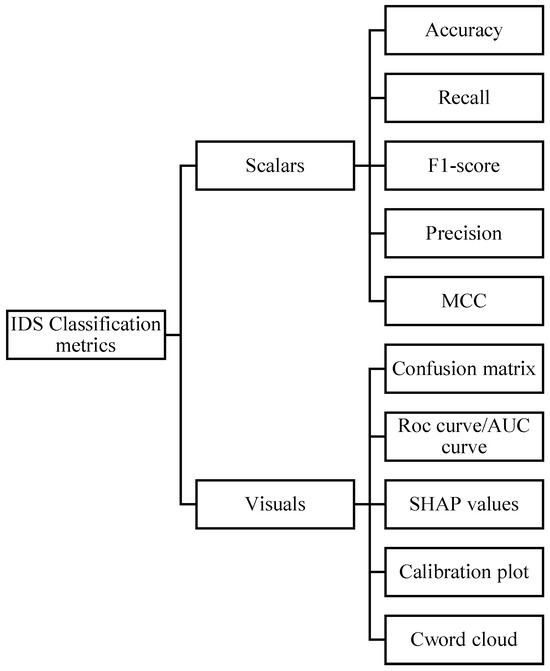
Figure 4. A typical classification metrics layout.

4. Experiments and Results

For demonstration purposes, we will use a simple LogisticRegression. We will use the saved sample dataset that was preprocessed in the previous section. We will set “Threat/Content Type” as a target with binary variables of values 1 and 0, representing “vulnerability” and “scan”, respectively. All other variables will remain as features.

In any model training, for instance, classification (for example, intrusion detection and threat analysis), building a model is only half the task. The other half is evaluating performance—ensuring that the model not only achieves high accuracy but also detects real threats reliably while minimizing false alarms.

Different metrics capture different aspects of performance. This section introduces key evaluation metrics, explains their theoretical basis, and demonstrates their application with Python 3.7. By combining explanation and practice, learners can connect concepts to real-world use.

4.1. Confusion Matrix

A confusion matrix is a classification matrix that summarizes predictions against actual outcomes. It reveals the types of errors a model makes. While evaluating a confusion matrix, some parameters are essential: true positive (TP), true negative (TN), false positive (FP), and false negative (FN). Table 3 illustrates confusion matrix elements, where the following applies:

Table 3. Illustration of confusion matrix elements.

Actual Values	Positive	TP	FN
	Negative	FP	TN
		Positive	Negative
		Predicted value

• TP (true positive): Threat correctly detected.
• TN (true negative): Normal traffic correctly classified.
• FP (false positive): Normal traffic flagged as a threat (false alarm).
• FN (false negative): Threat missed, classified as normal.

This metric is very important because it reveals what kinds of mistakes the model makes, not just how many mistakes were made.

Figure 5 offers a sample block of code developed to obtain a confusion matrix in a classification task.

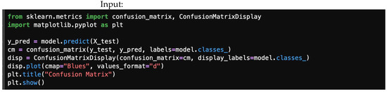
Figure 5. A sample block of code developed to obtain confusion matrix in classification task.

4.2. Accuracy

Accuracy is the simplest metric, referring to the rate of correct classifications achieved when comparing different methods on a naturally grouped dataset. It is measured by determining the accuracy of classifying new observations based on a rule developed using a labeled training set. It is formulated as shown in Equation (15):

$$Accuracy={\displaystyle \frac{TP+TN}{TP+TN+FP+FN}}$$

(15)

It is important to note that, in imbalanced datasets, accuracy can be misleading. A model that consistently predicts “normal” could achieve over 90% accuracy but fail to detect any threats. In Figure 6, an example of an accuracy code is given.

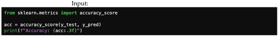
Figure 6. Accuracy code.

4.3. Precision, Recall, and F1-Score

Precision measures the accuracy of predicted threats, recall assesses the detection of actual threats, and F1-score balances both metrics. Trade-off highlights the inverse relationship between precision and recall, while macro and micro averaging provide different approaches to evaluating performance across classes. Equations (16)–(22) give a mathematical representation for precision, recall, F1-score, macro average precision, macro average recall, micro average precision, and micro average recall, respectively [22].

Precision: Of the predicted threats, how many were correct?

$$Precision={\displaystyle \frac{TP}{TP+FP}}$$

(16)

Recall (densitivity): Of the actual threats, how many were detected?

$$Recall={\displaystyle \frac{TP}{TP+FN}}$$

(17)

F1-score: Balances precision and recall (harmonic mean).

$$F1\_score=2\times {\displaystyle \frac{Precision\times Recall}{Precision+Recall}}={\displaystyle \frac{TP}{2TP+FP+FN}}$$

(18)

Macro averaging: Treats all classes equally.

$$Macro Average (precision)=\left({\displaystyle \frac{1}{N}}\right)\sum _i{\displaystyle \frac{T{P}_i}{T{P}_i+F{P}_i}}$$

(19)

$$Macro Average (Recall)=\left({\displaystyle \frac{1}{N}}\right)\sum _i{\displaystyle \frac{T{P}_i}{T{P}_i+F{N}_i}}$$

(20)

Micro averaging: Weighs results by class frequency.

$$Micro Average Precision={\displaystyle \frac{{\sum }_{i}T{P}_i}{{\sum }_{i}T{P}_i+{\sum }_{i}F{P}_i}}$$

(21)

$$Micro Average Recall={\displaystyle \frac{{\sum }_{i}T{P}_i}{{\sum }_{i}T{P}_i+{\sum }_{i}F{N}_i}}$$

(22)

All of these metrics can simply be obtained from a classification report, as shown in Figure 7, which shows a typical scalar metrics report. Note, they can also be calculated directly from the confusion matrix.

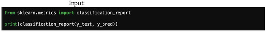
Figure 7. A typical scalar metrics report.

4.4. ROC Curve and AUC

The ROC (Receiver Operating Characteristic) curve visualizes the trade-off between the true-positive rate (TPR) and the false-positive rate (FPR) at different classification thresholds. A 0.5 on the ROC curve indicates random guessing, with no discrimination between positive and negative classes. Conversely, a value of approximately 1.0 suggests excellent discrimination, indicating that the model effectively distinguishes between positive and negative instances. This can be achieved using the following lines of code. We assume binary classification (number of classes equals 2). Input/output classifier visual measures are plotted in Figure 8 and Figure 9, representing visual measures for ROC curve and precision–recall curve, respectively. Figure 10 gives the logarithmic loss.

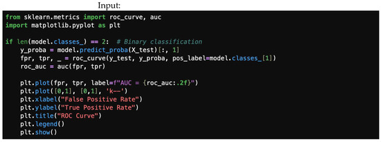
Figure 8. ROC curve.

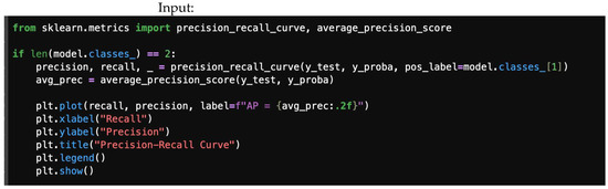
Figure 9. Precision–recall curve.

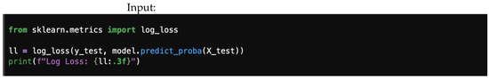
Figure 10. Logarithmic loss.

4.5. Precision–Recall Curve

The precision–recall curve is a graphical representation that illustrates the trade-off between precision and recall for different thresholds in a classification model. This metric is more informative than ROC when dealing with imbalanced datasets, as it focuses on the minority class (e.g., threat).

4.6. Logarithmic Loss (Log Loss)

Logarithmic loss, also known as cross-entropy loss, is a performance metric used to evaluate the accuracy of a classification model. It quantifies the difference between predicted probabilities and actual class labels, assessing how well the model predicts probabilities and penalizing confident but incorrect predictions, as shown in Equation (23).

$$logloss=-{\displaystyle \frac{1}{N}}\sum _i^N\sum _i^M{y}_i\log \left(p_{i,c}\right)$$

(23)

where

• $y_{i,c}$ is the true label indicator. It is 1 if the sample $i$ belongs to class c, and 0 otherwise.
• $p_{i,c}$ is the model’s predicted probability that sample $i$ belongs to class c. It is obtained from class predict_proba().

Here, small log loss implies better calibrated predictions, while large log loss implies overconfident mistakes.

4.7. Complete Example

Figure 11 shows the necessary libraries to import, giving all the necessary elements an author/developer needs to import before continuing.

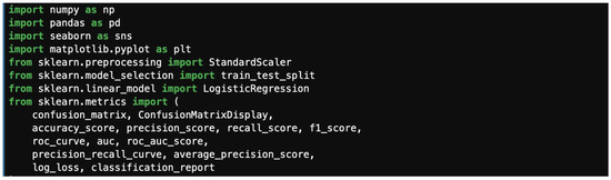
Figure 11. Necessary libraries to import.

Figure 12 shows the block of code to load the sample dataset. We define the target variable (y) as “Threat/Content Type”, drop it from the feature set X, and then standardize the features. This can all be achieved with the following block of code:

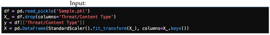
Figure 12. Block of code to load the dataset.

Figure 13 shows how to split a dataset into train and test sets. For demonstration, we will consider 80/20 (80% for training, and 20% for testing); this will be performed randomly. The random_state here is used for the reproducibility of the sample. This can be performed using the following code:

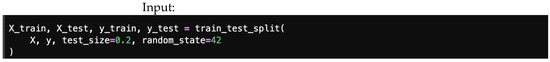
Figure 13. Splitting dataset into train and test sets.

Below, Figure 14 offers an example of how to check the size of the train and test split using either shape.

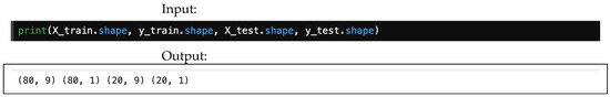
Figure 14. An example of how to check the sizes of the training and testing sets.

This illustration demonstrates the shape of the train and test split: the train features (X_train) consist of 80 rows by 9 columns, the train labels (y_train) are 80 rows by 1 column, the test features (X_test) are 20 rows by 9 columns, and the test labels (y_test) are 20 rows by 1 column. In total, there are 100 datapoints.

We instantiated the model (logistic regressor) using LogisticRegression(), and we trained the model using mode.fit(X_train, y_train). Figure 15 provides an example of a logistic regression predicted using model.predict(X_test).

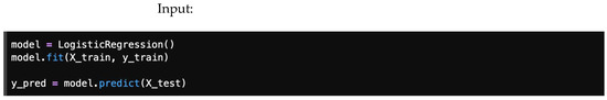
Figure 15. Logistic regression.

4.7.1. Confusion Matrix

Figure 16 illustrates a confusion matrix output library, giving a code to plot a confusion matrix for the predicted model, and Figure 17 shows a typical confusion matrix plot.

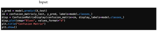
Figure 16. A confusion matrix output library.

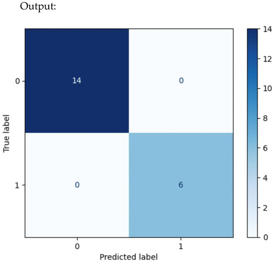
Figure 17. A typical confusion matrix plot.

4.7.2. Accuracy

Figure 18 gives an input/output sample for accuracy for the scalar’s precision, recall, and F1-score.

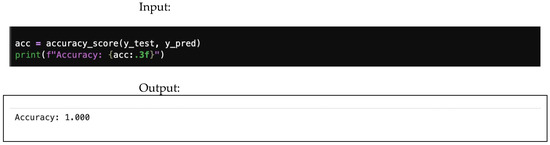
Figure 18. Accuracy input/output.

4.7.3. Precision, Recall, and F1-Score

Figure 19 outlines instruction(s) for classification scalar report.

Figure 19. Outline of instruction(s) for classification scalar report.

ML requires researcher’s understandability for modelling environmental settings. These vary to include the kind of dataset sample used, the classifier’s fit, and the hyperparameter configuration, in addition to the expected output performance ranges. Table 4 gives an example of such modelling output.

Table 4. Shows output values for precision, recall, F1-score, and the number of files needed to support output.

Metric	Precision	Recall	F1-Score	Support
0	1.00	1.00	1.00	14
1	1.00	1.00	1.00	6
Accuracy			1.00	20
Macro avg	1.00	1.00	1.00	20
Weighted avg	1.00	1.00	1.00	20

4.7.4. ROC Curve and AUC

ROC curve libraries are presented in Figure 20, and Figure 21 offers their ROC-AUC curve.

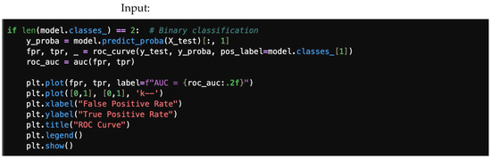
Figure 20. ROC curve libraries.

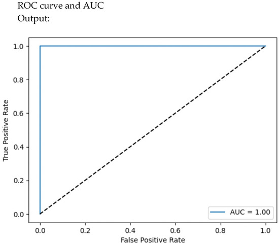
Figure 21. ROC-AUC curve.

4.7.5. Precision–Recall Curve

A precision–recall library is presented in Figure 22, and Figure 23 offers a precision–recall curve.

Figure 22. Precision/recall libraries.

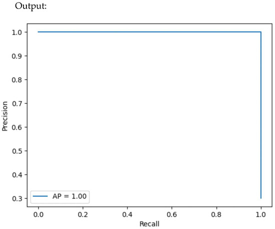
Figure 23. Precision–recall curve.

4.7.6. Logarithmic Loss (Log Loss)

Logarithmic loss library and output are shown in Figure 24.

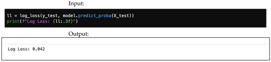
Figure 24. Logarithmic loss.

4.8. Handling Imbalance Data

Intrusion detection datasets are often highly imbalanced, with a vastly disproportionate number of “normal” instances compared to “attack” instances. Addressing this imbalance is crucial to prevent the model from becoming biased toward the majority class and underperforming on the minority (attack) class. This should always be performed after splitting the data into training and testing sets to avoid data leakage.

Objectives:

• Understand the problem of data imbalance.
• Learn various strategies to address imbalance (undersampling, oversampling, and hybrid).
• Implement common techniques like RandomOverSampler and SMOTE.
• Understand the importance of applying these techniques after splitting data into train/test sets.

Data imbalance can significantly affect the performance of machine learning models. How to handle it is by splitting the dataset library and resampling it, as shown in Figure 25.

Figure 25. Splitting the dataset library.

-

Step 1: Load data and check for imbalance.

First, read the data and check for class distribution.

-

Step 2: Split the data.

Split the dataset into training and testing sets, as shown in Figure 26.

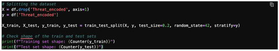
Figure 26. Splitting the dataset.

-

Step 3: Resample to address imbalance.

To address class imbalance, you can use techniques like oversampling the minority class or undersampling the majority class. Figure 27 offers a simple example using random oversampling on an imbalanced library. Meanwhile, Figure 28 illustrates the use of class distribution for train and test sets.

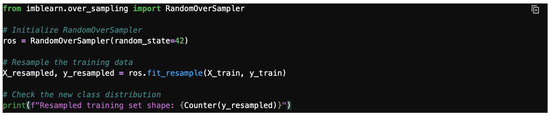
Figure 27. Imbalanced library.

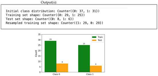
Figure 28. Class distribution for train and test. Note: You may need to install imblearn and collections packages.

4.8.1. Random Oversampling

This technique balances classes by randomly duplicating samples from the minority class. The input/output for the random oversampling is shown in Figure 29.

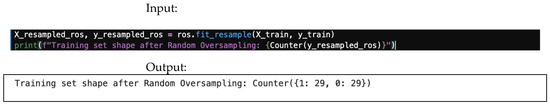
Figure 29. Random oversampling input/output.

4.8.2. SMOTE

SMOTE (synthetic minority oversampling technique) is a more advanced method that creates new synthetic samples for the minority class. By interpolating between existing minority instances in the feature space, SMOTE helps to create a more robust decision boundary and reduce overfitting. Figure 30 offers an example of SMOTE input/output.

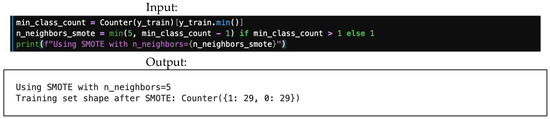
Figure 30. SMOTE input/output.

4.8.3. Random Undersampling (Use with Caution)

This technique balances data by randomly removing samples from the majority class. However, it should be used with caution, as it can lead to significant loss of information. Figure 31 demonstrates random undersampling input/output, while Figure 32 demonstrates balancing input/output.

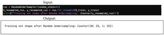
Figure 31. Random undersampling input/output.

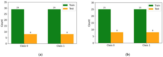
Figure 32. Balancing input/output. (a) Data balancing using oversampling/SMOTE. (b) Data balancing using random undersampling.

4.9. Sampling Dataset

This section consolidates the previously discussed steps into a single preprocessing pipeline. The code handles missing values by dropping rows, encodes categorical features, and applies standardization. The initial sample dataset with 100 datapoints is shown in Figure 33. Figure 34 shows a typical initial dataset sample code, and Figure 35 offers a typical initial dataset sample output.

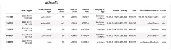
Figure 33. A typical initial dataset sample.

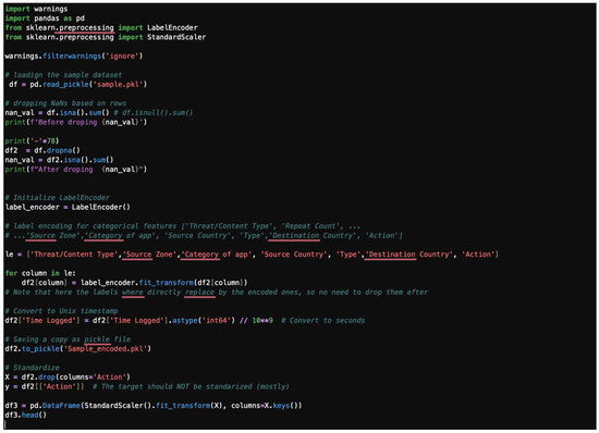
Figure 34. A typical initial dataset sample code.

Figure 35. A typical initial dataset sample output. Note: The Type column has a value of 0 throughout because all the values in the sample dataset are the same. The saved pickle file named “Sample_encoded.pkl” (df2) will be used for the remaining sections.

4.10. Advanced Feature Engineering

It is important to perform feature engineering on the entire dataset before splitting or to ensure that the logic is applied consistently to both the train and test sets. For simplicity, we will apply it to a copy of the original (pre-scaled) DataFrame for demonstration. In a real pipeline, these operations would be part of a custom transformer or applied before scaling. Let us revert to the one-hot encoded but unscaled DataFrame for feature engineering illustration, as some engineered features might be sensitive to the original scale. Therefore, we would re-apply scaling.

Creating new features can help models capture more complex patterns. For instance, generating polynomial features from existing ones can aid a model in learning nonlinear relationships within the data. Here is how to implement polynomial feature generation:

-

Step 1: Copy the DataFrame.

Start by copying the original DataFrame shown in Figure 36.

Figure 36. A typical DataFrame.

-

Step 2: Select features for polynomial transformation.

Choose the features you want to transform. For example, we can select “Action_encoded” and “Threat_encoded” presented in Figure 37, representing a typical threat encoded.

Figure 37. A typical threat encoded.

-

Step 3: Generate polynomial features.

Use PolynomialFeatures from sklearn 1.7 to create the new features. A polynomial feature illustration is shown in Figure 38. Polynomial features and their outputs are shown in Figure 39.

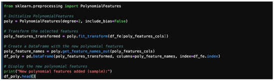
Figure 38. Polynomial features.

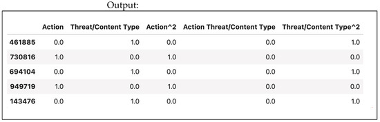
Figure 39. Polynomial features’ output.

By adding polynomial features, you enhance the model’s ability to learn complex relationships in the data. This transformation can significantly improve model performance, particularly for nonlinear patterns.

In addition to polynomial feature engineering, there are other methods, like logarithms and root transformations, as well as dimensionality reduction techniques (e.g., using PCA or t-SNE). Log and root transformations are used to stabilize variance and normalize skewed data, with log transformations compressing larger values, and root transformations reducing moderate skewness. Dimensionality reduction methods, such as PCA and t-SNE, aim to reduce the number of features while preserving essential information, thereby enhancing model performance and visualization.

4.11. Advanced Dimensionality Reduction

Reducing the number of features can improve model performance and reduce overfitting. Common techniques include the following:

Feature selection: Methods like SelectKBest or Random Forest feature importance rank features based on their statistical significance or contribution to the model’s predictions, allowing you to keep only the most impactful ones.

Feature extraction: Methods like Principal Component Analysis (PCA) transform the original features into a smaller set of new, uncorrelated components that preserve most of the original data’s variance. A typical dimensionality reduction sample code is given in Figure 40, and this code is followed by its plot in Figure 41, offering an example of dimensionality reduction output.

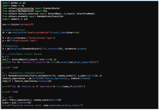
Figure 40. A typical dimensionality reduction code.

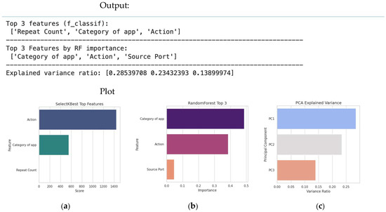
Figure 41. An example of dimensionality reduction output. (a) Filtering using selectKbest. (b) Feature importance using Random Forest. (c) PCA.

5. Discussion and Conclusions

Based on our re-run model to control the data leakage, we can generalize that cross-validation (k-fold CV), also named stratified k-fold CV, is more dependable than LOOV and is frequently used for k = 5 or 10. It aligns with the issues of unequal classification. In this instance, every sample was only checked once for validation, and every datapoint or sample was used for both training and validation. Keep in mind that k-fold CV equals LOOCV when k = n, which is equivalent to leave-one-out CV. Although computationally expensive, it is fairly accurate. With random divides, it can be performed repeatedly. When performing evaluations, this kind lowers variance. Additionally, nested CV is frequently used for both inner-loop hyperparameter adjustment (i.e., model selection with hyperparameter tuning) and outer-loop performance evaluation. It works incredibly well to stop data from leaking out of the validation set. The last type of CV is the Monte Carlo (Shuffle–Split) CV, which is distinguished by repeatedly splitting the datasets into training and testing at random. The test sets may overlap when using this strategy. With large datasets, however, it is quite helpful and adaptable, especially when the training/testing size is necessary. The following experiment concludes our generalization.

Often, IDS-based models need to strike a balance between variance (too complicated, overfitting) and bias (too simple, underfitting). This complexity is controlled by Random Forest depth. The Random Forest Classifier, whose complexity is controlled by the model’s depth, will be examined for demonstration purposes. This will serve as an example of overfitting, underfitting, and good fitting. Below, Figure 42 illustrates an overfitting/underfitting test.

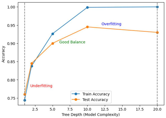
Figure 42. Illustration of overfitting/underfitting test.

Both training and testing accuracy are low at relatively low depths, suggesting underfitting. Training accuracy is almost flawless at an extremely high depth, but overfitting causes test accuracy to decline. Lastly, the optimal trade-off between mid-level depth, training, and testing accuracy is achieved. Table 5 below compares our methodology against the associated recently published articles.

Table 5. Comparison of our study findings with the recently published articles.

Article, Year	Algorithm(s)	Processes	Metrics	IDS	Imbalanced	Prediction	Learnability	IDAT	Best for
Wu, Y.; Zou, B.; Cao, Y., 2024 [23]	CNN, RNN, GANs	Summarize, preprocess, feature engineering, transform	Acc, recall, precision, F1, etc.	✓	✓	✓	🗶	🗶	Policy, strategy, framework
Wa’ad H. Aljuaid and Sultan S. Alshamrani, 2024 [24]	CNN, SMOTE	Balancing, feature selection	Acc, precision, recall,	✓	✓	✓	✓	🗶	Cloud-based, example/scenario
Fatima Isiaka, 2023–2024 [25]	CNN, RNN	Autoencoder-based	Precision, recall, etc.	✓	✓	✓	✓	🗶	Metrics discussion (scalar vs. visual)
Sajid, M.; Malik, K.R.; Almogren, A. et al., 2024 [26]	ML, DL, hybrid	Preprocess, explore	Acc, precision, F1-score, etc.	✓	✓	✓	🗶	🗶	Comparison-based models
A. Khan, M. S. Hossain, M. K. Hasan, et al., 2025 [27]	Review/survey	Explore emerging techs	FP, explore, F1, precision, etc.	✓	✓	✓	🗶	🗶	Justify metrics selection
Mert Nakıp, Erol Gelenbe, 2023 [28]	Supervised-based	Acquire online, auto-associate NN, trust evaluation	Acc, precision, recall, F1, etc.	✓	✓	✓	🗶	🗶	Useful in adaptive, streaming IDS
Jinxin Liu, Murat Simsek, Michele Nogueira, Burak Kantarci et al., 2023 [29]	Transfer arcitechure-based	Combine features and compare	F1-score	✓	✓	✓	🗶	🗶	Modern modeling, useful with metric trade-offs
Yifan Zeng et al., 2025 [30]	CNN, SC-CGAN	Generate, combine, oversample	Acc, F1, SHAP, LIME, cost-sensitive, attention	✓	✓	✓	🗶	🗶	Interpretability purposes
Ours, 2025	ML, DL, SMOTE, visualization, empirical	Preprocessing, undersampling, oversampling, feature engineering, dimensionality reduction	Acc, F1, precision, recall, ROC-AUC, visualization, confusion matrix, coding	✓	✓	✓	✓	✓	Modeling assessment, methodology development

For the sample dataset with only 100 datapoints, the target is “Thread/Content Type”. This target variable is highly correlated with other feature columns in the dataset. Figure 43 shows its correlation with other related features.

Figure 43. Contributed correlation features on “Thread/Content Type” as a target feature.

For this reason, the prediction accuracy is 1.00. Table 6 illustrates the SMOTE parameters, and Table 7 shows how logistic regression reflected the hyperparameter settings for our re-run reported models.

Table 6. SMOTE parameters.

Parameter	Value
sampling_strategy	‘auto’
random_state	47
k_neighbors	5

Table 7. Logistic regression.

Parameter	Value
penalty	‘l2’
tol	0.0001
C	1
solver	‘lbfgs’
max_iter	100
intercept_scaling	1

Note: All of these parameters are default values; they were not tuned, due to the model’s performance.

Figure 44 gives the model performance on the entire dataset (complete dataset).

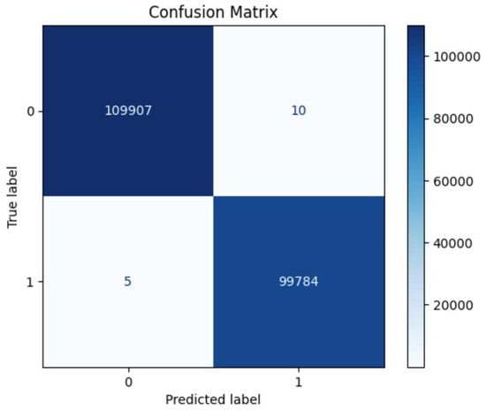
Figure 44. Confusion matrix indication for the complete dataset.

There was a little difference in model performance regarding the dataset size. For example, in the following, the model was trained with different datapoints and evaluations; the R² scores are shown in Table 8.

Table 8. Concluded classification report using the whole/subset dataset and based on “Thread/Content Type”.

Metric	Precision	Recall	F1-Score	Support	Test Size	Accuracy
0	1.00	1.00	1.00	109,917	10,000	1.000000
1	1.00	1.00	1.00		20,000	1.000000
accuracy			1.00	209,706	30,000	1.000000
macro avg	1.00	1.00	1.00	209,706	40,000	0.999875
weighted avg	1.00	1.00	1.00	209,706	50,000	1.000000
weighted avg	1.00	1.00	1.00	209,706	60,000	0.999917
					70,000	1.000000
					80,000	1.000000
					90,000	0.999833
					100,000	0.999750
					110,000	0.999909
					120,000	0.999792
					130,000	0.999962
					140,000	0.999929
					150,000	1.000000
					160,000	0.999844
					170,000	0.999853
					180,000	0.999889
					190,000	0.999921

The authors argue that the study agreed with [31,32,33,34] in terms of IDS-imbalanced assessments, and our study leads the rest of the linked works by innovating its empirical methodology and findings diversity supported by case examples. Table 1 and Table 5 can easily guide a researcher to choose his/her methodology by evaluating imbalanced datasets and the domain in which the study takes place.

RQ1: 

How do IDC assessments direct the classifiers’ analysis domains in relation to cybersecurity aspects?

Our findings show that IDC assessments offer a systematic framework for assessing classifiers, in addition to providing accuracy, including visual (such as confusion matrices, ROC/PR curves, and word cloud plots) and scalar (such as precision, recall, and F1-score) metrics. The trade-offs between false positives, false negatives, and interpretability—all of which are crucial in IDS systems—are highlighted by this multifaceted evaluation, which guides classifier analysis toward a more impartial judgment.

RQ2: 

What kind of output(s) dominates IDS classification when exploring the dataset?

Scalar performance indicators, including F1-score and recall, predominate in IDS evaluations, according to the comparison analysis, particularly in unbalanced environments, where accuracy might be deceptive. However, because they provide interpretability and threshold-independent insights, visual outputs like PR curves and confusion matrix explanations are increasingly used in conjunction with scalar metrics. When combined, these results offer a more thorough comprehension of classifier behavior in IDS settings.

RQ3: 

What implications do these findings have for IDS policy and strategy?

According to the results, IDS policy should use a framework that incorporates both interpretable visual diagnostics and balanced scalar metrics rather than depending only on one performance parameter, like accuracy. This guarantees system deployment that is transparent and reliable. From a policy standpoint, implementing such a framework promotes repeatability, makes cross-institutional benchmarking easier, and aids in decision-making in settings where misclassifications or false negatives pose serious security threats.

Robust assessment metrics, cost-sensitive learning, and resampling are necessary for IDS on unbalanced datasets. The most successful approaches are hybrid ones, practically speaking, (SMOTE plus boosting, and GANs with ensembles); however, evaluations must concentrate on PR-AUC, F1, G-mean, MCC, and recall rather than accuracy.

The environmental setup for the models was based on Python 3.7 64-bit for our large dataset calculations and analysis; Jupyter Notebook3 with Anacoda 3 2020 Navigator represented a great base. The raw or filthy dataset was cleaned using influential machine learning approaches, and the features that support the IDS candidate target were chosen. The dataset was used in this work to guide the modeling process and form the projected classifier depending on the target class. To build the dataset that offers the best input attributes that pro-support each output, deeper preprocessing operations were used.

A researcher’s study direction can be developed in many ways. First, the researcher can use unified IDS distributed learning with imbalanced network traffic. Second, the researcher can examine why IDS misclassifies rare attacks by testing explainable artificial intelligence. Thirdly, the researcher can ensure adversarial robustness by making sure IDS can handle imbalance and withstand evasive attacks.

References

- Uddin, A.; Aryal, S.; Bouadjenek, M.R.; Al-Hawawreh, M.; Talukder, A. Hierarchical classification for intrusion detection system: Effective design and empirical analysis. Ad Hoc Netw. 2025, 178, 103982. [Google Scholar] [CrossRef]
- Alotaibi, M.; Mengash, H.A.; Alqahtani, H.; Al-Sharafi, A.M.; Yahya, A.E.; Alotaibi, S.R.; Khadidos, A.O.; Yafoz, A. Hybrid GWQBBA model for optimized classification of attacks in Intrusion Detection System. Alex. Eng. J. 2025, 116, 9–19. [Google Scholar] [CrossRef]
- Suarez-Roman, M.; Tapiador, J. Attack structure matters: Causality-preserving metrics for Provenance-based Intrusion Detection Systems. Comput. Secur. 2025, 157, 104578. [Google Scholar] [CrossRef]
- Shana, T.B.; Kumari, N.; Agarwal, M.; Mondal, S.; Rathnayake, U. Anomaly-based intrusion detection system based on SMOTE-IPF, Whale Optimization Algorithm, and ensemble learning. Intell. Syst. Appl. 2025, 27, 200543. [Google Scholar] [CrossRef]
- Araujo, I.; Vieira, M. Enhancing intrusion detection in containerized services: Assessing machine learning models and an advanced representation for system call data. Comput. Secur. 2025, 154, 104438. [Google Scholar] [CrossRef]
- Devi, M.; Nandal, P.; Sehrawat, H. Federated learning-enabled lightweight intrusion detection system for wireless sensor networks: A cybersecurity approach against DDoS attacks in smart city environments. Intell. Syst. Appl. 2025, 27, 200553. [Google Scholar] [CrossRef]
- Le, T.-T.; Shin, Y.; Kim, M.; Kim, H. Towards unbalanced multiclass intrusion detection with hybrid sampling methods and ensemble classification. Appl. Soft Comput. 2024, 157, 111517. [Google Scholar] [CrossRef]
- He, H.; Garcia, E.A. Learning from imbalanced data. IEEE Trans. Knowl. Data Eng. 2009, 21, 1263–1284. [Google Scholar] [CrossRef]
- Othman, S.M.; Ba-Alwi, F.M.; Alsohybe, N.T.; Al-Hashida, A.Y. Intrusion detection model using machine learning algorithm on Big Data environment. J. Big Data 2018, 5, 34. [Google Scholar] [CrossRef]
- Rao, Y.N.; Babu, K.S. An Imbalanced Generative Adversarial Network-Based Approach for Network Intrusion Detection in an Imbalanced Dataset. Sensors 2023, 23, 550. [Google Scholar] [CrossRef]
- Sun, Z.; Zhang, J.; Zhu, X.; Xu, D. How Far Have We Progressed in the Sampling Methods for Imbalanced Data Classification? An Empirical Study. Electronics 2023, 12, 4232. [Google Scholar] [CrossRef]
- El-Gayar, M.M.; Alrslani, F.A.F.; El-Sappagh, S. Smart Collaborative Intrusion Detection System for Securing Vehicular Networks Using Ensemble Machine Learning Model. Information 2024, 15, 583. [Google Scholar] [CrossRef]
- Gong, W.; Yang, S.; Guang, H.; Ma, B.; Zheng, B.; Shi, Y.; Li, B.; Cao, Y. Multi-order feature interaction-aware intrusion detection scheme for ensuring cyber security of intelligent connected vehicles. Eng. Appl. Artif. Intell. 2024, 135, 108815. [Google Scholar] [CrossRef]
- Gou, W.; Zhang, H.; Zhang, R. Multi-Classification and Tree-Based Ensemble Network for the Intrusion Detection System in the Internet of Vehicles. Sensors 2023, 23, 8788. [Google Scholar] [CrossRef]
- Moulahi, T.; Zidi, S.; Alabdulatif, A.; Atiquzzaman, M. Comparative Performance Evaluation of Intrusion Detection Based on Machine Learning in In-Vehicle Controller Area Network Bus. IEEE Access 2021, 9, 99595–99605. [Google Scholar] [CrossRef]
- Wang, W.; Sun, D. The improved AdaBoost algorithms for imbalanced data classification. Inf. Sci. 2021, 563, 358–374. [Google Scholar] [CrossRef]
- Abedzadeh, N.; Jacobs, M. A Reinforcement Learning Framework with Oversampling and Undersampling Algorithms for Intrusion Detection System. Appl. Sci. 2023, 13, 11275. [Google Scholar] [CrossRef]
- Sayegh, H.R.; Dong, W.; Al-Madani, A.M. Enhanced Intrusion Detection with LSTM-Based Model, Feature Selection, and SMOTE for Imbalanced Data. Appl. Sci. 2024, 14, 479. [Google Scholar] [CrossRef]
- Palma, Á.; Antunes, M.; Bernardino, J.; Alves, A. Multi-Class Intrusion Detection in Internet of Vehicles: Optimizing Machine Learning Models on Imbalanced Data. Futur. Internet 2025, 17, 162. [Google Scholar] [CrossRef]
- Zayid, E.I.M.; Humayed, A.A.; Adam, Y.A. Testing a rich sample of cybercrimes dataset by using powerful classifiers’ competences. TechRxiv 2024. [Google Scholar] [CrossRef]
- Faul, A. A Concise Introduction to Machine Learning, 2nd ed.; Chapman and Hall/CRC: New York, NY, USA, 2025; pp. 88–151. [Google Scholar] [CrossRef]
- Tharwat, A. Classification assessment methods. Appl. Comput. Inform. 2018, 17, 168–192. [Google Scholar] [CrossRef]
- Wu, Y.; Zou, B.; Cao, Y. Current Status and Challenges and Future Trends of Deep Learning-Based Intrusion Detection Models. J. Imaging 2024, 10, 254. [Google Scholar] [CrossRef]
- Aljuaid, W.H.; Alshamrani, S.S. A Deep Learning Approach for Intrusion Detection Systems in Cloud Computing Environments. Appl. Sci. 2024, 14, 5381. [Google Scholar] [CrossRef]
- Isiaka, F. Performance Metrics of an Intrusion Detection System Through Window-Based Deep Learning Models. J. Data Sci. Intell. Syst. 2023, 2, 174–180. [Google Scholar] [CrossRef]
- Sajid, M.; Malik, K.R.; Almogren, A.; Malik, T.S.; Khan, A.H.; Tanveer, J.; Rehman, A.U. Enhancing Intrusion Detection: A Hybrid Machine and Deep Learning Approach. J. Cloud Comput. 2024, 13, 1–24. [Google Scholar] [CrossRef]
- Neto, E.C.P.; Iqbal, S.; Buffett, S.; Sultana, M.; Taylor, A. Deep Learning for Intrusion Detection in Emerging Technologies: A Comprehensive Survey and New Perspectives. Artif. Intell. Rev. 2025, 58, 1–63. [Google Scholar] [CrossRef]
- Nakıp, M.; Gelenbe, E. Online Self-Supervised Deep Learning for Intrusion Detection Systems (SSID). arXiv 2023, arXiv:2306.13030. Available online: https://arxiv.org/abs/2306.13030 (accessed on 1 September 2025).
- Liu, J.; Simsek, M.; Nogueira, M.; Kantarci, B. Multidomain Transformer-based Deep Learning for Early Detection of Network Intrusion. arXiv 2023, arXiv:2309.01070. Available online: https://arxiv.org/abs/2309.01070 (accessed on 10 September 2025). [CrossRef]
- Zeng, Y.; Jin, R.; Zheng, W. CSAGC-IDS: A Dual-Module Deep Learning Network Intrusion Detection Model for Complex and Imbalanced Data. arXiv 2025, arXiv:2505.14027. Available online: https://arxiv.org/abs/2505.14027 (accessed on 10 September 2025).
- Chen, Y.; Su, S.; Yu, D.; He, H.; Wang, X.; Ma, Y.; Guo, H. Cross-domain industrial intrusion detection deep model trained with imbalanced data. IEEE Internet Things J. 2022, 10, 584–596. [Google Scholar] [CrossRef]
- Sangaiah, A.K.; Javadpour, A.; Pinto, P. Towards data security assessments using an IDS security model for cyber-physical smart cities. Inf. Sci. 2023, 648, 119530. [Google Scholar] [CrossRef]
- Disha, R.A.; Waheed, S. Performance analysis of machine learning models for intrusion detection system using Gini Impurity-based Weighted Random Forest (GIWRF) feature selection technique. Cybersecurity 2022, 5, 1–22. [Google Scholar] [CrossRef]
- Sarhan, M.; Layeghy, S.; Portmann, M. Towards a standard feature set for network intrusion detection system datasets. Mob. Networks Appl. 2022, 27, 357–370. [Google Scholar] [CrossRef]
Disclaimer/Publisher’s Note: The statements, opinions and data contained in all publications are solely those of the individual author(s) and contributor(s) and not of MDPI and/or the editor(s). MDPI and/or the editor(s) disclaim responsibility for any injury to people or property resulting from any ideas, methods, instructions or products referred to in the content. |
© 2025 by the authors. Licensee MDPI, Basel, Switzerland. This article is an open access article distributed under the terms and conditions of the Creative Commons Attribution (CC BY) license (https://creativecommons.org/licenses/by/4.0/).