Article

A Zero-Shot Image Classification Method of Ship Coating Defects Based on IDATLWGAN

1
School of Mechanical Engineering, Jiangsu University of Science and Technology, Zhenjiang 212100, China
2
Industrial Technology Research Institute of Intelligent Equipment, Nanjing Institute of Technology, Nanjing 211167, China
*
Author to whom correspondence should be addressed.
Coatings 2024, 14(4), 464; https://doi.org/10.3390/coatings14040464
Submission received: 29 February 2024 / Revised: 28 March 2024 / Accepted: 10 April 2024 / Published: 11 April 2024
(This article belongs to the Special Issue The Present Status of Thermally Sprayed Composite Coatings)

Abstract

:
In recent years, the defect image classification method based on deep transfer learning has been widely explored and researched, and the task of source and target domains with the same painting defect image class has been solved successfully. However, in real applications, due to the complexity and uncertainty of ship painting conditions, it is very likely that there are unknown classes of painting defects, and the traditional deep learning model cannot identify a few classes, which leads to model overfitting and reduces its generalization ability. In this paper, a zero-shot Image classification method for ship painting defects based on IDATLWGAN is proposed to identify new unknown classes of defects in the target domain. The method is based on a deep convolutional neural network combined with adversarial transfer learning. First, a preprocessed ship painting defect dataset is used as input for the domain-invariant feature extractor. Then, the domain invariant feature extractor takes domain invariant features from the source and target domains. Finally, Defect discriminators and domain alignment discriminators are employed to classify the known categories of unlabeled defects and unknown categories of unlabeled defects in the target domain and to further reduce the distance between the edge distributions of the source and target domains. The experimental results show that the proposed model in this paper extracts a better distribution of invariant features in the source and target domains compared to other existing transfer learning models. It can successfully complete the migration task and accurately recognize the painting defects of known categories and new unknown categories, which is a perfect combination of intelligent algorithms and engineering practice.

1. Introduction

Ship coating runs through the entire shipbuilding process as one of modern shipbuilding’s three central process pillars [1]. Ship hull surface coating can effectively prevent all parts of the ship from being corroded by the atmosphere and seawater. Still, it also has anti-fouling, beautification, decoration, and other special functions [2]. The coating quality is directly related to the ship’s construction cycle and maintenance costs, as well as an essential factor affecting the hull’s corrosion resistance and the ship’s service life [3]. However, in the process of ship coating construction, due to the joint influence of many factors such as process parameters, internal and external environment, and coating quality, many different types of coating defects such as sagging, blistering, cracking, delamination, etc. will occur [4], These coating defects not only affect the ship’s beauty but also affect the quality of the ship’s coatings, reduce the ship’s anti-fouling and anti-corrosion function, which affects the service life of the ship [5]. Therefore, in the whole process of ship construction, it is crucial to carry out intelligent identification of painting defects and feedback on painting information to improve the quality of ship painting, prolong the service life of ships, and enhance the market competitiveness of shipbuilding enterprises.
Feature extraction is to extract effective feature information from images, which is usually used as the basis of image classification [6,7]. Domestic and foreign research scholars have carried out a lot of studies on image classification algorithms; Liu et al. [8] combined multi-dimensional convolutional layers with an attention mechanism model to realize the satisfactory classification performance of CNNs in the framework of small-sample learning, which was used to solve the small-sample problem in hyperspectral image classification; Shi et al. [9] proposed an efficient binary network search method to design lightweight binary networks, and used it for image classification tasks in CIFAR10 and CIFAR100; Jin et al. [10] mapped visual feature vectors obtained from fine-tuned ConvNeXt network and semantic vectors obtained from BioBert coding into a common metric space, and proposed a new double-weighted metric loss function for metricizing the distance between images and labels. Zheng et al. [11] used the graph Laplace matrix of the learning dictionary to preserve the locality information, used the label information of the atoms to construct the label embedding term, and verified that the optimal coding coefficients obtained from locality-based and label-based reconstruction are effective for image classification. Currently, traditional coating defect identification mainly relies on professionals to detect the coating quality and record the types and grades of defects through their professional knowledge and work experience. This method is slow [12], inefficient [13], and affected by the subjective factors of the inspectors, resulting in low reliability of the detection results. With the popularization and development of modern manufacturing concepts and intelligent manufacturing technology in ship construction, people gradually begin to apply intelligent technologies and algorithms to the ship construction process. Still, there are few reports on the research and application of intelligent detection of painting defects based on image recognition.
In recent decades, deep learning methods represented by convolutional neural networks have attracted extensive attention from relevant researchers engaged in manufacturing industries with their ability to extract [14] effective high-level features end-to-end automatically and have achieved great success in the fields of natural language processing [15], image recognition [16] and speech recognition [17]. However, there are still many shortcomings that need to be addressed. First, deep learning methods rely on large-scale and high-quality labeled training samples. Still, it is difficult to collect enough labeled training data, and the cost of labeling is too high to guarantee the generalization performance of deep learning models in real industrial environments [18]; second, existing deep learning models usually assume that the training sample dataset and the test sample dataset must be independently and identically distributed, which is unrealistic [19]. According to the research of domestic and foreign scholars, deep transfer learning methods can relax this restriction by effectively solving new tasks in the target domain with knowledge learned from the relevant source domain, effectively solving the above problems, and improving the generalization performance of the target model [20]. Kuang et al. [21] proposed a class-imbalanced adversarial transfer learning (CIATL) network for cross-domain troubleshooting by embedding class-imbalanced learning into the adversarial training process and bi-level adversarial transfer learning, including marginal and conditional distribution adaptation performed. The effectiveness and generalization of the method are verified on a planetary gearbox rig. Lu et al. [22] propose transfer subspace learning for cross-resolution image classification, introducing transfer subspace learning techniques and applying low-rank and sparse constraint matrices. The accuracy of the method was verified on various real image datasets. Li et al. [23] proposed a two-stage transfer adversarial network to construct a new deep transfer learning model based on the adversarial learning strategy, followed by an unsupervised convolutional self-encoder model with silhouette coefficients for multiple novel fault detection of rotating machinery, to solve the fault diagnosis migration task with multiple new faults in the target domain. Xu et al. [24] proposed a new geometric migration metric learning method that integrates pairwise constraints, joint distributional adaption, and manifold regularization into a unified optimization function, making full use of their complementary properties to improve SAR ship classification performance. Conducted in both zero-labeled sample (ZLS) and small-labeled sample (SLS) tasks, experiments show that the proposed method outperforms most state-of-the-art methods. Li et al. [25] proposed a deep learning model based on a multi-scale feature extraction module for steel surface defects, deepening the backbone network by improving the Efficient Feature Fusion (EFF) and Bottleneck modules. The effectiveness of the designed module and method is verified on the public NEU-DET dataset.
In summary, deep transfer learning can be broadly categorized into five types: weighted instance-based migration [26], model parameter-based migration [27], relationship-based migration [28], feature-based migration [29], and adversarial-based migration [30] (ADTL). Among them, adversarial-based deep migration methods are most widely used due to their practicality and good migration results [31].
Although machine learning models based on deep transfer learning algorithms have achieved great success in many fields, such as machinery fault diagnosis [32], image classification [33], etc., most of the existing transfer learning methods are based on the assumption that the source and target domains share the same labeling space, namely, the source and target domains share the same number of categories [34]. However, in practical applications, there will likely be unknown class painting defects due to the complexity and uncertainty of ship painting conditions. These newly appeared unknown class painting defects in the target domain cannot be aligned with the source domain samples due to the lack of samples during the training process in the source domain and are often identified as known class defects in the source domain, which reduces the generalization performance of existing deep transfer learning models. Therefore, detecting unknown class painting defects in the target domain is an important task for intelligent inspection of ships.
To address the aforementioned task, an adversarial migration framework model consisting of domain-invariant feature extractor, Defect discriminators, and domain alignment discriminators is proposed to utilize the known class defects in the source domain to accurately classify the unknown class defects in the target domain. The contributions of this paper are summarized as follows:
(1)
This paper proposes a new zero-sample classification method for ship painting defects based on deep adversarial transfer learning based on Wasserstein GAN (IDATLWGAN) for identifying new unknown class painting defects in the target domain.
(2)
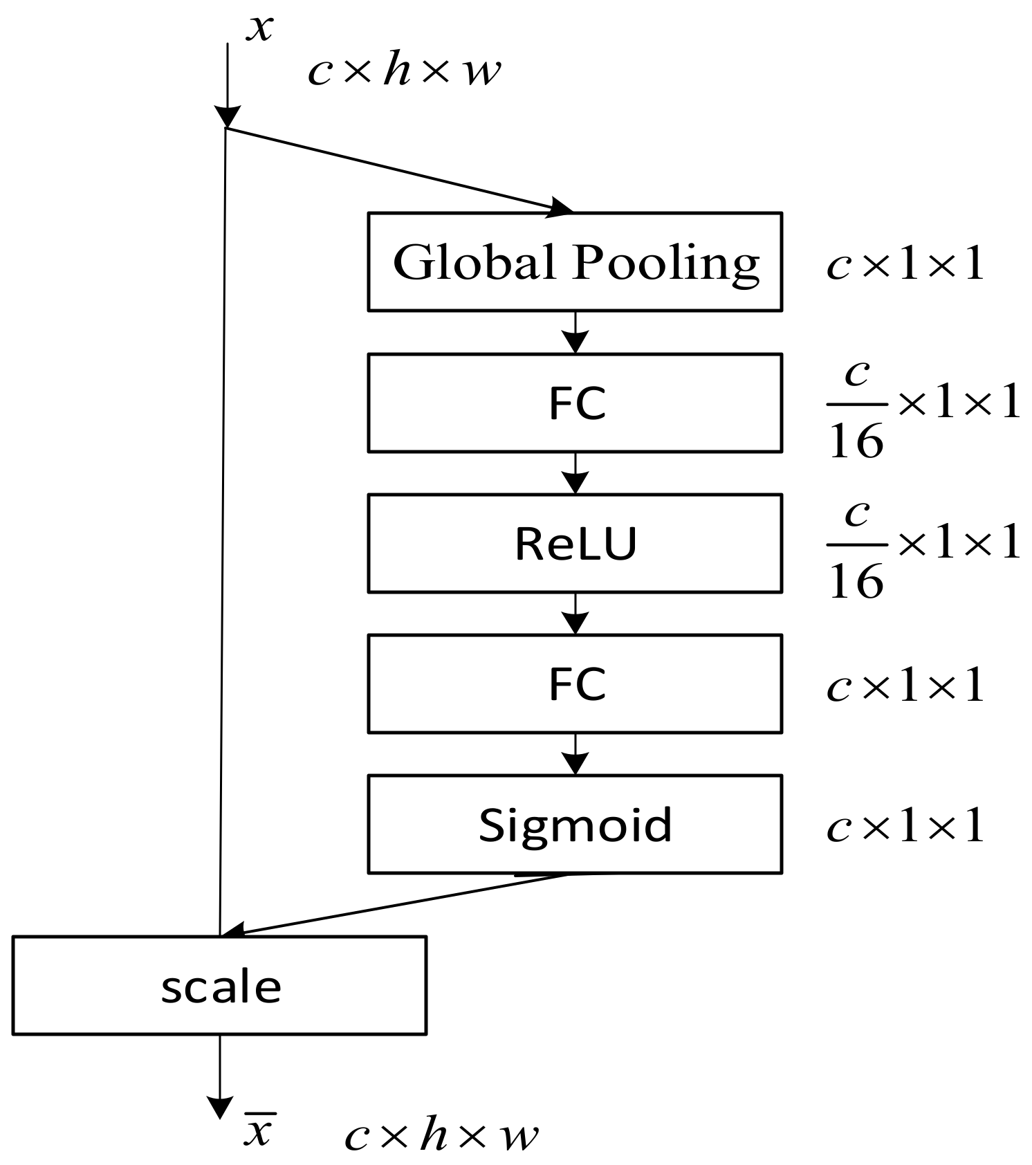
In this paper, the Squeeze-and-Excitation (SE) module is introduced in the domain-invariant feature extractor and used in the transfer learning task, which is more capable of using global information to acquire important domain-invariant features selectively and suppress less useful ones.
(3)
Domain alignment discriminators are introduced and used in a deep transfer model, which learns domain-invariant and class-separation features to classify defects accurately through two-stage adversarial training.
The experiments show that the proposed IDATLWGAN model can better perform the migration task and accurately identify known classes of painting defects and new unknown classes of painting defects on the ship painting defects dataset compared to other existent transfer learning models.

2. Theoretical Background

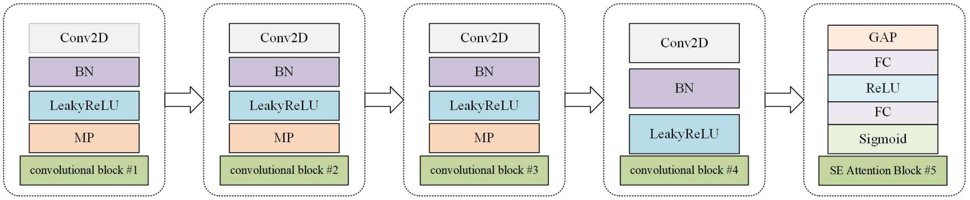
2.1. Classification Domain CNN Structure

Convolutional Neural Networks (CNN) are feed-forward neural networks which is more widely used in pattern classification because they avoid the complex pre-processing of the image and can be directly input to the original image [35]. CNN in the classification field consists of three parts: convolutional layer, pooling layer, and fully connected (FC) layer. The convolutional layer is the core layer used to build CNN, and its role is to extract image features, as defined in Equation (1).
y m l = σ ( x l 1 · k m l · χ + b m l )
where x l 1 shows the feature map of the l 1 layer input, · χ shows the convolution operation, k m l and b m l show the convolution kernel and bias unit corresponding to the l layer m-channel, respectively, σ shows the activation function, and y m l shows the convolution output of the l layer m-channel.
The pooling layer is used to summarize the feature map features and reduce the spatial size of the feature map. It is defined as shown in Equation (2).
g m l = V R ( y m l ( U c ) )
where U c shows the location coordinates, V R shows the pooling operation, and g m l shows the pooled output of the l layer m-channel.
The fully connected (FC) layer acts as a “classifier” in the whole CNN. While operations such as convolutional and pooling layers map the original data to the hidden feature space, the fully connected layer maps the learned “distributed feature representation” to the sample labeling space.

2.2. SE Attention Mechanisms

The SE module was proposed by Jie Hu et al. [36]. The relationship between channels is constructed by introducing Squeeze and Excitation operations, where the feature map is compressed into a c × 1 × 1 feature vector z c by global average pooling in the Squeeze ( F s q ( · ) ) phase, as shown in Equation (3).
z c = F s q ( u c ) = 1 H × W i = 1 H j = 1 W u c ( i , j )
In the Excitation ( F e x ( · ) ) phase, a weight vector S for a channel is learned to be generated using a fully connected layer ( W 1 , W 2 ) and a nonlinear activation function ( R e L U , S i g m o i d ). as shown in Equation (4).
s = F e x ( z , W ) = σ ( g ( ( z , W ) ) = σ ( W 2 δ ( W 1 z ) )
A hyperparameter r exists between the two fully connected layers, and in this paper, r is taken as 16. vector z   (   c × 1 × 1   ) changes its dimension to (   c / r × 1 × 1   ) after passing through the first fully connected layer and then to (   c × 1 × 1   ) again after passing through the second fully connected layer. The generated weight vectors S (   c × 1 × 1   ) are applied to each channel on the feature map U (   c × h × w   ) to weigh the features of different channels. In this way, the SE module can adaptively select and emphasize the important features and improve the discriminative ability of the features, thus improving the model’s performance. Its structure is shown in Figure 1.

2.3. Adversarial-Based Domain Adaptation Training

The Generative Adversarial Networks (GAN) designed by GoodFellow [37] contains two models: a generator and a discriminator. During adversarial training, the goal of generator G is to generate real graph deception slices to deceive discriminator D to maximize the classification error. The goal of discriminator D is to distinguish the picture generated by generator G from the actual picture to minimize the classification error. The model is optimized by a minimal-extremum game of G and D. The GAN optimization objective function V ( D ,   G ) is denoted as shown in Equation (5).
min G   max D V ( D , G ) = E x   ~ P d a t a ( x ) [ log D ( x ) ] + E z ~ P z ( z ) [ log ( 1 D ( G ( z ) ) ) ]
where log ( D ( x ) ) is the cross entropy between [ 1 , 0 ] T and [ D ( x ) , 1 D ( x ) ] T . l o g ( 1 D ( G ( z ) ) ) is the cross entropy between [ 0 , 1 ] T and [ D ( G ( z ) ) , 1 D ( G ( z ) ) ] T .
In domain adaptation, given a predefined N s R source domain dataset D s = { ( x s i , y s i ) } i = 1 N s with labels y s i and N t R unlabeled target domain datasets D t = { x t i } i = 1 N t , the source and target domains share the same feature space ( D s , D t χ a ) and labeling space χ b . Still, the source and target domains have different distributions. The task of the domain adaptation algorithm is to learn a classifier f : α β that utilizes the source domain dataset D s with labels y s i to predict the labels of the target domain dataset D t .
The domain adaptive neural network (DANN) designed by Yaroslav Ganin [38] et al. introduced the adversarial idea into the field of transfer learning for the first time. In domain-adaptive adversarial training, the domain-invariant feature extractor learns high-level domain-invariant features from D s and D t . It characterizes them to be passed to the domain discriminator, which constantly updates the difference between D s and D t and calculates the loss. The domain discriminator training goal is to classify D s and D t accurately. In contrast, the feature extractor is trained with the opposite goal (due to the presence of the gradient inversion layer), creating an adversarial relationship. The difference between D s and D t is minimized by backpropagation, and then the domain-invariant feature extractor learns high-level domain-invariant features.

3. Proposed Methodology

3.1. Problem Definition and Symbolic Description

This paper researches the problem of classifying new unknown class painting defects without labels in different labeling spaces. Specifically, supervised training data and unsupervised test data used to drive the painting defect classification model are collected from the shipyard’s painting logbook, construction accounts, and painting process database. Before elaborating on the IDATLWGAN framework, the readability of the content is enhanced by defining the relevant problems through symbols or formulas.
First of all, for deep transfer learning (DTL), there are two basic concepts: domain D and task T. Among them, the domain D consists of two components: the feature space χ and the edge probability distribution P ( X ) , as shown in Equation (6).
D = { χ , P ( X ) }
where X = { x 1 , x 2 , , x n } χ denotes an n-dimensional vector; P ( X ) denotes the marginal probability distribution of the feature space χ.
A given predefined N s R source domain dataset D s = { ( x s i , y s i ) } i = 1 N s with labels y s i and N t R target domain datasets D t = { x t i } i = 1 N t without labels y t i (typically, 1 N t N s ) exists. The source and target domains share the same feature space (namely, D s , D t χ ) but have different edge probability distributions (namely, P s ( D s ) P t ( D t ) ). If X s X t and (or) P s ( D s ) P t ( D t ) , the source and target domain distributions are different, (namely, D s D t ). Also, task T consists of two parts: the category labeling space Y and the conditional probability distribution P ( Y | X ) , as shown in Equation (7).
T = { Y , P ( Y | X ) }
where Y denotes a category labeling space, the conditional probability distribution P ( Y | X ) denotes the target prediction function C ( · ) of the feature space.
Since the source and target domain datasets have the same classes in the existing deep transfer learning models, their class labeling space is also the same. However, unlabeled unknown class defects appear in the target domain, thus Y s Y t . In addition, in this paper, the target domain D t contains two components, namely, n j k unlabeled known class painting defects samples and n j n unlabeled unknown class painting defects samples. n j k and n j n are satisfied n j k + n j n = n t . Finally, the high-level invariant feature vectors extracted by the DCNN model from the source and target domains are defined as V s i ( x s i , y s i ) and V t i ( x t i ) . This paper shows the Important variables and function symbols and their definitions in Table 1.

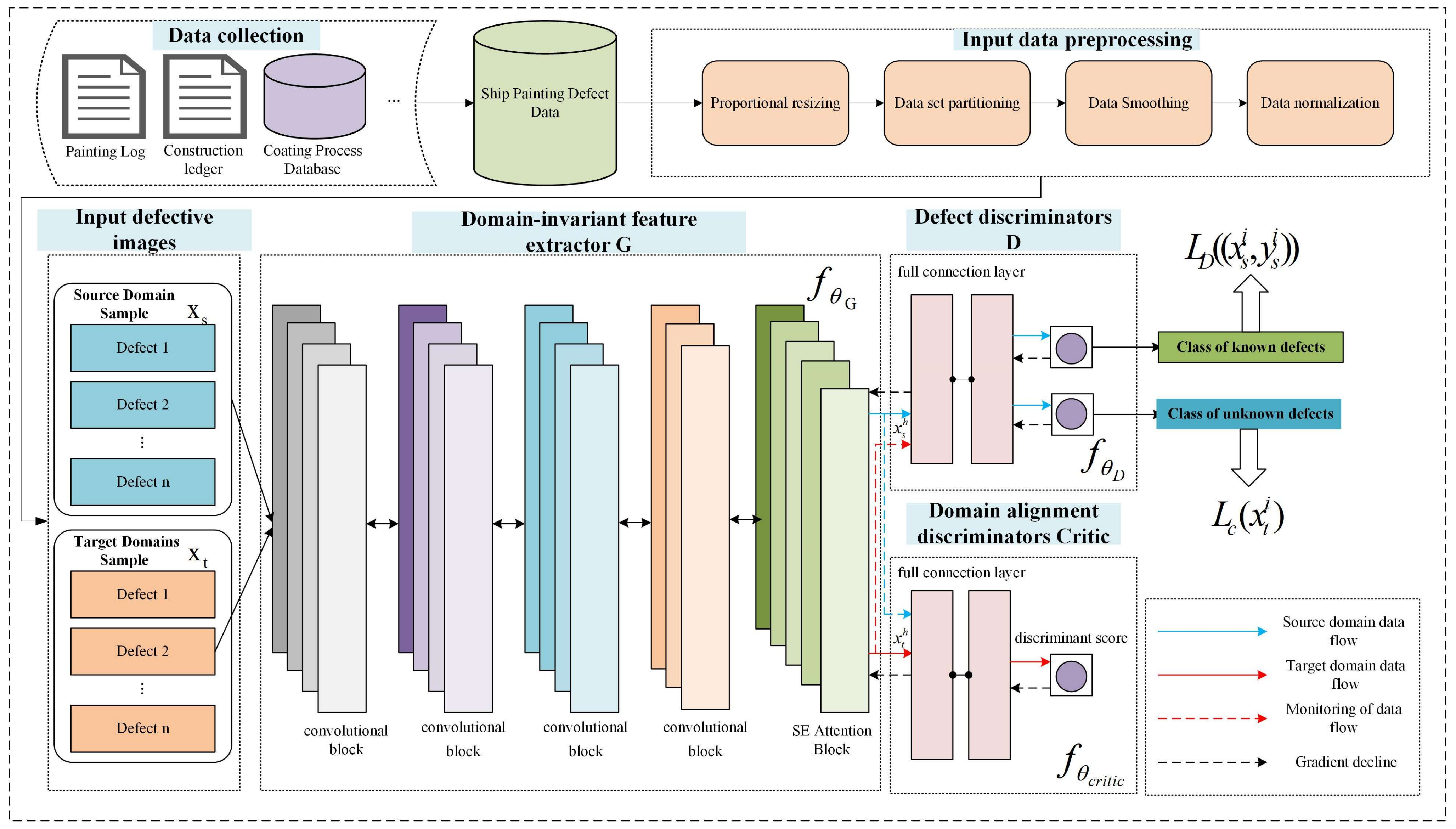
3.2. Overall Network Framework

The IDATLWGAN ship painting defect zero-sample intelligent classification method based on IDATLWGAN proposed in this paper consists of domain-invariant feature extractor G, Defect discriminator D, and domain alignment discriminators critic. The model structure is shown in Figure 2. The acquired ship painting defects dataset is first preprocessed (proportional resizing, data set partitioning, data smoothing, and data normalization) in this work. Then, the preprocessed dataset is divided into source and target domain data. The migratable features of the source and target domain data can be represented as x s h = G ( x s i ) and x t h = G ( x t i ) . The feature extractor G consists of convolutional blocks and SE attention blocks, which are designed to extract high-level domain-invariant features from the defect images of the source and target domains, and its structure and network parameters are shown in Figure 3 and Table 2. Defect discriminator D and domain alignment discriminators critic is employed to classify the known unlabeled defects and unknown unlabeled defects in the target domain by the learned high-level domain invariant features and to reduce further the distributional difference between the edge probability distributions P s ( D s ) and P t ( D t ) in the source and target domains. The domain-aligned discriminator critic is connected to the feature extractor G by the FC layer, gradient reversal layer (GRL), and sigmoid function completion.
The training strategy for the IDATLWGAN model is an adversarial learning mechanism, which is a min-max game between domain-invariant feature extractor G, Defect discriminators D, and domain alignment discriminators critic.

3.3. Loss Function

The purpose of iterative adversarial training of the IDATLWGAN model is to minimize the loss function. Its loss function has four constituents, as shown in Equation (8).
min θ D , θ G { L D ( x s i , y s i ) + λ L c ( x t i ) + η max θ C r i t i c [ L w d ( x s , x t ) ρ L g r a d ] }
where λ, η, and ρ are the weight balance coefficients of the loss function, the hyperparameters λ and η are used to determine the hyper coefficients of the confusion level of the source and target domains, and 1 and 2 denote the standard cross-entropy loss function of Defect discriminators model D for fast classification of unlabeled known defective samples in the target domain and the binary cross-entropy loss function for identifying new unlabeled unknown painting defects in the target domain, as shown in Equations (9) and (10).
L D ( x s i , y s i ) = log [ D ( ( V s i ( x s i , y s i ) ) ) ]
L c ( x t i ) = ζ log ( p ( y = n + 1 | x t i ) ) ( 1 ζ ) log ( 1 p ( y = n + 1 | x t i ) )
where D ( ( V s i ( x s i , y s i ) ) ) denotes the probability of defective samples in the source domain, and V s i ( x s i , y s i ) denotes the high-level domain invariant feature vector extracted by the DCNN model from the source domain, as shown in Equation (11).
V s i ( x s i , y s i ) = p ( y = 1 | x s i ) p ( y = 2 | x s i ) p ( y = n | x s i ) = 1 j = 1 n e z j e z 1 e z 2 e z n
where p ( y = n | x s i ) denotes the probability that the input sample x s i in the target domain is classified as a known unlabeled defect class j { 1 , 2 , , n } , z j = V s ( V s i ( x s i , y s i ) ) j denotes the jth value, V s i ( x s i , y s i ) denotes the normalization term, and n is the number of types of defects in the known class.
Since a known class defect sample will have a higher probability of being recognized as a known class defect than a new unlabeled unknown defect sample, a threshold parameter ζ ( 0 < ζ < 1 ) is chosen to determine whether a sample belongs to a known defect sample or a new unknown class defect sample to quantify the pseudo-decision boundaries between the known class defect category and the unknown class defect category. The role of the threshold parameter is shown in Figure 4. If the probability p ( y = n + 1 | x t i ) exceeds the threshold ζ , the sample is recognized as a new unknown class defective sample. This paper sets the threshold parameter ζ to 0.5, as shown in Figure 4.
Domain alignment discriminators loss L w d ( x s , x t ) is used to compute the Wasserstein distance between edge probability distributions P s ( D s ) and P t ( D t ) , as shown in Equation (12).
L w d ( x s , x t ) = E x p s [ f θ C r i t i c ( x ) ] E x p t [ f θ C r i t i c ( x ) ] = 1 N s x s X s f θ C r i t i c ( f θ e ( x s ) ) 1 N t x t X t f θ C r i t i c ( f θ e ( x t ) )
where L w d denotes the domain alignment discriminative loss of the source domain data X s and the target data X t .
Inspired by Wasserstein Generative Adversarial Networks-Gradient Penalty (WGAN-GP), this paper adds a gradient penalty term L g r a d (gradient penalty, GP) in L w d ( x s , x t ) , which is used to solve the problem with Lipschitz constraints such as vanishing or exploding gradients, as shown in Equation (13).
L g r a d = ( x h f ( x h ) 2 1 ) 2
where x h denotes the vector of high-level invariant feature representations of the source and target domains.
In summary, based on the proposed adversarial training network architecture, the optimization objective of domain-invariant feature extractor G is to minimize L D ( x s i , y s i ) and domain alignment discriminators loss L w d ( x s , x t ) and maximize L c ( x t i ) at the same time. The optimization objective of Defect discriminators model D is to minimize L D ( x s i , y s i ) and L c ( x t i ) at the same time. The optimization objective of domain alignment discriminators critic is to minimize L w d ( x s , x t ) ρ L g r a d and L c ( x t i ) at the same time. Therefore, the proposed network optimization problem is shown in Equations (14)–(16).
θ ^ G = arg { min θ G L D ( x s i , y s i ) , min θ G L w d ( x s i , x t i ) , max θ G L c ( x t i ) }
θ ^ D = arg { min θ D L D ( x s i , y s i ) , min θ D L c ( x t i ) }
θ ^ C r i t i c = arg { min θ C r i t i c [ L w d ( x s , x t ) ρ L g r a d ] , min θ C r i t i c L c ( x t i ) }
where θ ^ G , θ ^ D , and θ ^ C r i t i c denote the optimal estimated parameter values for θ G , θ D , and θ C r i t i c , respectively. At each training turn, the parameters of the model are updated, as shown in Equations (17)–(19).
θ G θ G α 1 θ G [ L D ( x s , y s ) λ L c ( x t ) + η L w d ( x s , x t ) ]
θ D θ D α 1 θ D [ L D ( x s , y s ) + λ L c ( x t ) ]
θ C r i t i c θ C r i t i c α 1 θ C r i t i c [ λ L c ( x t ) ] α 2 θ C r i t i c [ L w d ( x s , x t ) ρ L g r a d ( x h ) ]
where α 1 denotes the learning rate of the domain-invariant feature extractor G and Defect discriminator model D, and α 2 denotes the learning rate of the domain alignment discriminators critic.

3.4. Training Process Optimization and Implementation Details

Based on the above loss function, to solve the parameter updating and minimal maximal optimization problems of the unsupervised transfer learning Back Propagation (BP) algorithm, this paper brings in the Gradient Reversal Layer (GRL), which has two forms, namely, Forward Propagation and Back Propagation, and its mathematical expressions are shown in Equations (20) and (21). For forward propagation, GRL is a constancy mapping. For backward propagation, GRL extracts the gradient from the next layer and multiplies it by a negative hyperparameter −α (α > 0) to pass it to the previous layer. Thus, GRL has no parameters that need to be predefined or trained. In this paper, the GRL module is introduced between domain-invariant feature extractor G and Defect discriminators model D during backpropagation, which ensures that the feature distributions of different domains are indistinguishable as a way of facilitating domain-invariant feature extractor G and Defect discriminators model D to learn high-level domain-invariant features with an adversarial training strategy.
G λ ( x ) = x
d G λ d x = α I
where I is the unit matrix and α denotes the penalty coefficient, as shown in Equation (22). In this paper, it is simplified and set to 1.
α = 2 1 + exp ( γ · p ) 1
where γ is the hyperparameter, set to 10 in this paper, and p denotes the relative value of the iteration process, namely, the ratio of the current number of iterations to the total number of iterations.
In addition to this, momentum-based optimization algorithms such as Adam’s algorithm perform worse due to the instability of the discriminator loss, whereas the RMSProp optimizer performs well even in volatile conditions, so we use the RMSProp optimizer for stochastic gradient descent optimization of the model parameters. The number of epochs is 50. In this work, the initial learning rate is set to 0.001, and the decay rate of the learning rate equals 0.1.

3.5. Training Process

The overall training process of the proposed IDATLWGAN model is shown in Algorithm 1, and the whole network training process is divided into the following eight steps:
  • STEP1: Data Collection: Original ship painting defect data sets are collected through the shipyard’s painting log, construction ledger, and painting process database.
  • STEP2: Data Preprocessing: Image preprocessing consists of four steps, namely, proportional resizing, data set partitioning, data smoothing, and data normalization.
  • STEP3: The ship painting defects training set after STEP2 processing is divided into source and target domain data.
  • STEP4: The source and target domain defective training sets are used together as input to the domain-invariant feature extractor G. The extractor extracts high-level domain-invariant features from the defective images of the source and target domains.
  • STEP5: The Defect discriminator D and domain alignment discriminators critic is employed to classify the known unlabeled defects and unknown unlabeled defects in the target domain by the learned high-level domain-invariant features and to reduce further the distributional differences between the edge probability distributions of the source and target domains.
  • STEP6: Update parameters θ G , θ D , and θ C r i t i c of domain-invariant feature extractor G, Defect discriminator model D, and domain alignment discriminators critic, respectively.
  • STEP7: Repeat STEP4~STEP6 to iteratively update the parameters of each module through the adversarial training strategy until convergence, and store all the parameters to obtain the trained optimal estimated parameter values  θ ^ G , θ D , and θ C r i t i c .
  • STEP8: All test datasets are used to test and validate the validity of the IDATLWGAN model.
Algorithm 1: The overall training process for the IDATLWGAN model
Require: Source and target domain datasets D s and D t ; small batch size n; learning rate α1, α2; number of updates of domain alignment discriminators critic in each iteration; and weight balance coefficients λ, η, and ρ for each loss function.
Initialize hyperparameters for different networks θ ^ G , θ D , and θ C r i t i c .
While i < Maximum number of iterations or convergence of parameters of each module do
   1:  { ( x s i , y s i ) } i = 1 n P s ( D s ) ←Randomized small batch sampling from a real ship painting defect source domain dataset.
   2:  { x t i } i = 1 n P t ( D t ) ←Random small batch sampling from a real ship painting defects target domain dataset.
   3:  For i = 1, …, n D  do
   4:   x s h f θ e ( x s ) P s ( D s ) , x t h f θ e ( x t ) P t ( D t )
   5:  Sampling from pairs x s h and x t h yields x r h
   6:   x h { x s h , x t h , x r h }
   7:   L g r a d ( x h f ( x h ) 2 1 ) 2
   8:   L c ( x t i ) ζ log ( p ( y = n + 1 | x t i ) ) ( 1 ζ ) log ( 1 p ( y = n + 1 | x t i ) )
   9:    L w d ( x s , x t ) 1 N s x s X s f θ C r i t i c ( f θ e ( x s ) ) 1 N t x t X t f θ C r i t i c ( f θ e ( x t ) )
   10:    θ C r i t i c θ C r i t i c α 1 θ C r i t i c [ λ L c ( x t ) ] α 2 θ C r i t i c [ L w d ( x s , x t ) ρ L g r a d ( x h ) ]
   11:  End For
   12:   θ D θ D α 1 θ D [ L D ( x s , y s ) + λ L c ( x t ) ]
   13:   θ G θ G α 1 θ G [ L D ( x s , y s ) λ L c ( x t ) + η L w d ( x s , x t ) ]
End While
Output Optimal parameter estimates for each module θ ^ G , θ D , and θ C r i t i c .
End

4. Experiments Setup and Results

4.1. Description of the Dataset

In this work, a total of 6 typical ship painting defect types are analyzed, including three types of painting defects in the wet film state: sagging (SA), orange skin (OS), blistering (BL), and three types of painting defects in the dry film state: cracking (CR), pinholing (PH), delamination (DF). To avoid the problem of category imbalance, which leads to a transfer learning model, results in overfitting of the model, and significantly reduces generalization performance, the number of samples of each painting defect category is set to 600 in this paper. Among them, the amount of sample data in the source domain of various ship painting defect categories is set to 300, while the amount of data in the target domain of the training set and the test set is set to 150. Table 3 lists the details of the ship painting defect dataset. Since the original ship painting defects images collected were of different sizes and proportions, all the images were resized to 3 × 128 × 128 before carrying out the experiments. The preprocessed ship painting defects dataset was randomly divided into a training set and test set in the ratio of 0.7:0.3. In addition to the above preprocessing techniques, data smoothing technique (Gaussian filtering) and data normalization technique are used in this paper to remove the image noise, improve the image quality and ensure that each feature is in the same dimension, respectively, which significantly improves the convergence speed and prediction performance of the neural network. Based on previous research work, this paper uses the min-max normalization technique to scale the defective image pixels from [0, 255] to [0, 1].

4.2. Experimental Environment

The hardware platform used in this experiment is an 11th Gen Intel ® Core TM i7-11800H @ 2.3 GHz (Intel, Santa Clara, CA, USA) with NVIDIA GeForce RTX 3060 Laptop GPU (NVIDIA, Santa Clara, CA, USA) and 16.0 GB RAM. The programming language is Python (version 3.8.4).

4.3. Evaluation Metrics

Different quantitative evaluation metrics are used in the experimental part of the experiment to accurately and comprehensively assess the overall generative performance of the model and measure the performance of the comparison model for the migration task on various defect categories in the ship painting defect dataset. In this paper’s experiments, four usual evaluation metrics in the confusion matrix are used to quantitatively analyze the model performance: accuracy, precision, recall, and F1 score. The binary classification confusion matrix is shown in Table 4.
Accuracy and recall are complementary; the higher these metrics are, the better. Accuracy is the most intuitive model performance metric, and precision is the ratio of correctly predicted positive observations to total predicted positive observations. The F1 score is the reconciled mean of the lookup accuracy and recall. It considers both precision rate and recall rate and is often used as a statistical metric to evaluate the performance of a classifier. These evaluation metrics are defined as shown below:
Accuracy = T P + T N T P + T N + F P + F N
Pr ecision = T P T P + F P
Recall = T P R = T P T P + F N
F 1 -score = 2 × Precision   ×   Recall Precision + Recall = 2 2 T P + F P + F N

4.4. Experimental Results and Analysis

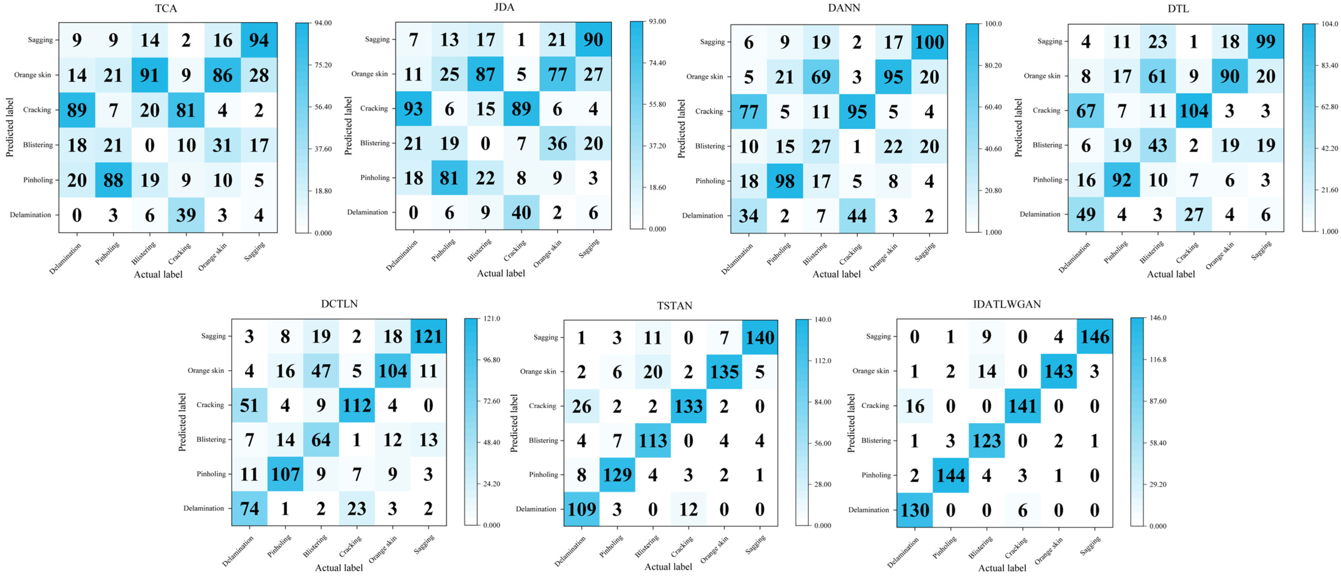
4.4.1. Performance Comparison of Different Transfer Learning Models on Different Painting Defect Categories

To further demonstrate the effectiveness and superiority of the method proposed in this paper, different existing transfer learning models such as Transfer Principal Component Analysis (TCA), Joint Distribution Adaptive (JDA), Domain Adaptive Neural Network (DANN), Deep Transfer Learning (DTL), Deep Confrontation Migration Learning Network (DCTLN), and Two-Stage Migration Confrontation Network (TSTAN) are compared with the IDATLWGAN model proposed in this paper. The number of parameters and training time for each model are shown in Table 5. Comparison experiments with various defect categories in different transfer learning models in a real ship painting defect dataset are shown in Table 6. The bold values indicate the maximum values of the evaluation metrics in different migration models. Table 6 shows the average training results of the five-fold cross-validation to reduce the randomness of the data.
Compared with other existing transfer learning models, although the IDATLWGAN model proposed in this paper has lower F1 scores of 0.013 and 0.008 for sagging defects (SA) and cracking defects (CR) compared with TSTAN and DCTLN, respectively, the F1-score are generally higher in other defects. Meanwhile, defects are much higher than in other transfer learning models in other evaluation metrics (precision and recall). It reflects the unstable performance and the low performance of other transfer learning models when facing different defects. Based on the analysis of the above results, it can be concluded that the overall performance of the IDATLWGAN model proposed in this paper is better than that of other transfer learning models on the ship painting defects dataset.

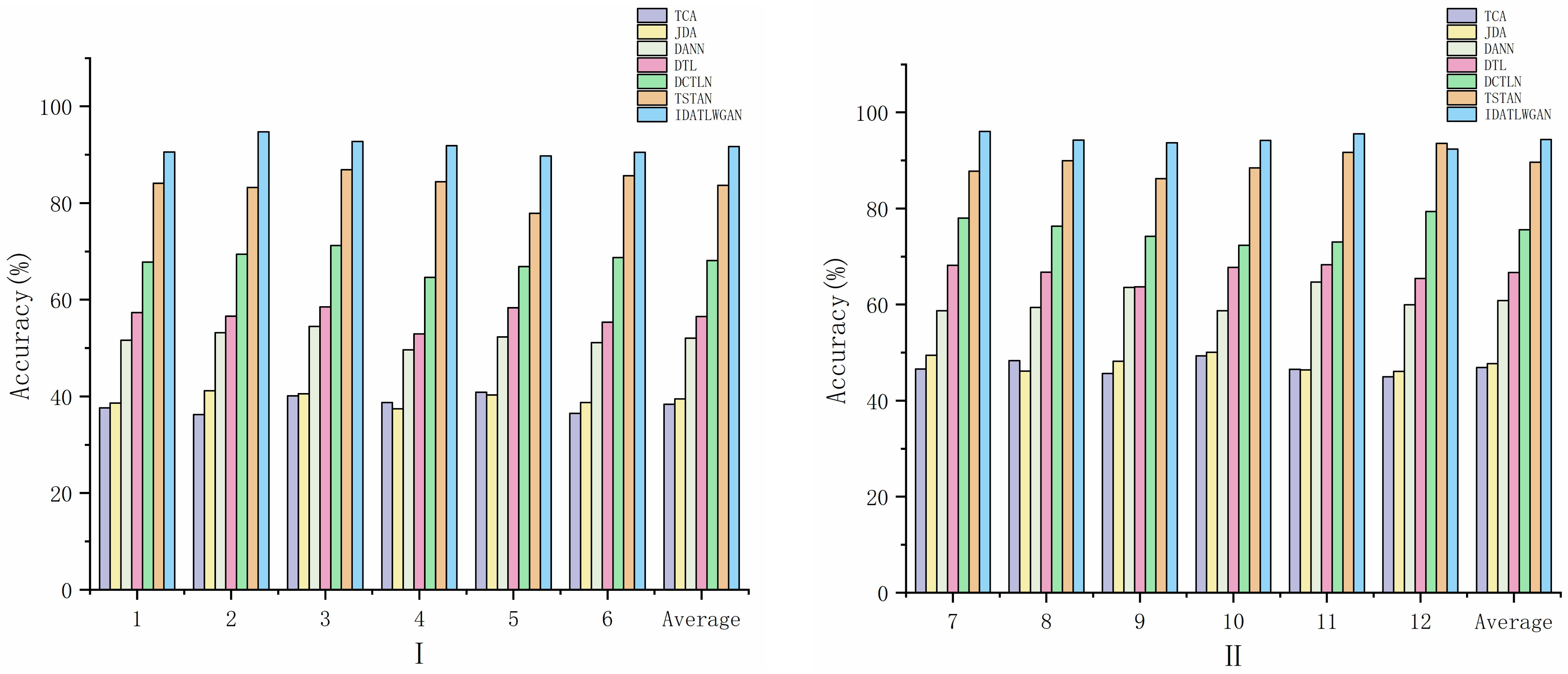
4.4.2. Performance Comparison of Different Transfer Learning Models on Different Migration Tasks

In this section, to validate the stability and reliability of the proposed IDATLWGAN model, two groups of experiments, I and II, are designed, each with six migration tasks, as shown in Table 7. Sagging (SA), orange skin (OS), blistering (BL), cracking (CR), pinholes (PH), and delamination (DF) were collected to construct the source and target domain datasets. The collected painting defects were generated at different air temperatures (15 °C, 25 °C, and 35 °C) and relative humidities (50% and 60%) as shown in Table 8. In Experiment I, the source domain dataset is labeled SA, OS, CR, and PH, and the target domain dataset has unlabeled SA, OS, CR, PH, and unlabeled unknown classes BL and DF. Six migration tasks were designed in scenarios with the same temperature and different humidities, different temperatures and different humidities, and different temperatures and same humidities, and a cross-validation strategy was used to validate the IDATLWGAN model’s performance, migration task 1 (namely, A→C) represents the migration task from the source domain defective dataset under condition A to the target domain defective dataset under condition C. The other tasks are similar. The other tasks are similar. To further reduce the experiment’s randomness and verify the reliability of the IDATLWGAN model, Experiment II is designed using the cross-validation strategy. In Experiment II, the source domain dataset has labeled SA, OS, CR, and PH; for the target domain dataset, three tasks contain unlabeled SA, OS, CR, PH, and BL, and the other tasks contain unlabeled SA, OS, CR, PH, and DF.
The experimental results of all the transfer learning tasks on the ship defects dataset are summarized in Table 9 and Figure 5, and the bold values indicate the maximum accuracy values in different transfer learning models on different transfer tasks. Compared with the traditional methods such as TCA and JDA, the existing deep learning methods (DANN, DTL, DCTLN) have slightly higher average accuracy due to their relatively good feature extraction ability to recognize a small number of unknown unlabeled category defects. Due to their powerful feature extraction ability, the TSTAN and IDATLWGAN models have high average accuracy. The quantitative experimental results show that although the accuracy of the TSTAN model is higher than that of the IDATLWGAN model by 1.19% on task 12 (namely, F→B), the accuracy on the remaining tasks is still low. The proposed IDATLWGAN model achieves an average accuracy of 91.71 and 94.35 on the ship defects dataset in the two sets of experiments I and II, which are both higher than the other comparative methods and can effectively detect unknown class painting defects on ships without labels in the target domain.
Confusion matrices are often used to visually represent the number of accurate predictions and the number of misclassifications for each class in the test results and to interpret this result at the class level. Figure 6 shows the confusion matrices for all transfer learning methods on Task 4. The horizontal axis represents the true attributes, and the vertical axis represents the predicted state of the data. The main diagonal elements indicate the number of samples correctly categorized by each defective class. In contrast, besides the main diagonal elements, the remaining elements indicate the number of samples incorrectly categorized into other defective classes. TCA and JDA are entirely unable to identify the unlabeled unknown classes BL and DF due to their limited extraction capabilities. They are not able to efficiently isolate defective samples from other classes. DANN, DTL, DCTLN, and TSTAN are poor at recognizing defective categories compared to IDATLWGAN. TSTAN, with limited feature extraction capability, can only achieve about 83.33% accuracy due to the shadow structure. The results show that IDATLWGAN performs well in painting defect classification.
To present the transfer results intuitively, a visual data dimensionality reduction algorithm-t distribution stochastic neighborhood embedding algorithm (t-SNE) is used to present the learned feature distribution. For example, Task 9 compares the transferable characteristics of the TCA, JDA, DANN, DTL, DCTLN, TSTAN, and IDATLWGAN methods. Severe features are aliasing in the transferable features of TCA and JDA. There is a severe mixing of known painting defect samples from the source and target domains with the new unmarked painting defect samples, which are not separated from the painting defect samples. Therefore, when the model is trained using the prior knowledge of the source domain, the unmarked target samples cannot be effectively separated using TCA and JDA. The transferable features learned by DANN, DTL, and DCTLN need to be more effectively separated. Specifically, although the known painting defect samples have been transferred from the source domain to the target domain, the new unmarked painting defect samples are still mixed in the known painting defect samples. TSTAN and IDATLWGAN can not only cluster the known painting defect samples of the source and target domains clearly but also separate the new unmarked painting defect samples from the known painting defect samples, but the IDATLWGAN clearly has fewer new unlabeled painting defect samples mixed with known painting defect samples compared to TSTAN, so IDATLWGAN can effectively transfer features from the source domain to the target domain and detect new unlabeled painting defect samples in the unlabeled target domain. This result also illustrates that IDATLWGAN has higher transfer accuracy and better performance than other methods.

5. Conclusions and Future Work

In this paper, a zero-sample classification method for ship painting defects based on IDATLWGAN is proposed, which can not only effectively identify the known class of unlabeled painting defects from the source domain to the target domain but also accurately identify the unknown class painting defects that are unlabeled in the target domain at the same time, which can effectively prevent the model from overfitting as well as improve the model’s generalization ability. The experimental results show that compared with other existing transfer learning models, the model proposed in this paper extracts a better distribution of invariant features in the source and target domains, and its Accuracy, F-Score, Precision, and Recall values are significantly higher than those of other models. With the above results, using the IDATLWGAN model to classify ship painting defects can complete the migration task and accurately identify the known classes of painting defects and new unknown class painting defects, a perfect combination of intelligent algorithms and engineering practice. It has high engineering research value and application prospects.
Currently, it is proved experimentally that the transfer learning method can be used for ship painting to identify unknown class painting defects, but experiments have not yet been conducted on other scenarios to illustrate the general applicability of the transfer learning method; therefore, in the follow-up work, we will consider diagnosing unknown faults on troubleshooting to validate the effectiveness and robustness of the proposed method.
In addition, for real-time or resource-constrained applications, techniques to optimize the computational efficiency of the proposed model are investigated. Explore the integration of real-time monitoring systems for continuous defect detection during ship painting. Develop methods to provide explanations and interpretations for the model’s decisions.

Author Contributions

H.B. revised the paper and completed it and financial support, T.Y. wrote the first draft of the paper, C.H., X.Z. and Z.G. collected and sorted the data, Z.Y. financial support and investigation. Y.T. investigation. All authors have read and agreed to the published version of the manuscript.

Funding

The authors gratefully acknowledge the financial support from the Ministry of Industry and Information Technology High-Tech Ship Research Project: Research on the Development and Application of a Digital Process Design System for Ship Coating (No.: MC-202003-Z01-02), the National Defense Basic Scientific Research Project: Research and Development of an Intelligent Methanol-Fueled New Energy Ship (No.: JCKY2021414B011), and the RO-RO Passenger Ship Efficient Construction Process and Key Technology Research (No.: CJ07N20).

Institutional Review Board Statement

Not applicable.

Informed Consent Statement

Not applicable.

Data Availability Statement

The data that support the findings of this study are available from the corresponding author upon reasonable request.

Conflicts of Interest

The authors declare that there are no conflicts of interest regarding the publication of this work.

References

  1. Bu, H.; Yuan, X.; Niu, J.; Yu, W.; Ji, X.; Lyu, Y.; Zhou, H. Ship Painting Process Design Based on IDBSACN-RF. Coatings 2021, 11, 1458. [Google Scholar] [CrossRef]
  2. Yuan, X.; Bu, H.; Niu, J.; Yu, W.; Zhou, H. Coating matching recommendation based on improved fuzzy comprehensive evaluation and collaborative filtering algorithm. Sci. Rep. 2021, 11, 14035. [Google Scholar] [CrossRef]
  3. Bu, H.; Hu, C.; Yuan, X.; Ji, X.; Lyu, H.; Zhou, H. An Image Generation Method of Unbalanced Ship Coating Defects Based on IGASEN-EMWGAN. Coatings 2023, 13, 620. [Google Scholar] [CrossRef]
  4. Ma, H.; Lee, S. Smart System to Detect Painting Defects in Shipyards: Vision AI and a DeepLearning Approach. Appl. Sci. 2022, 12, 2412. [Google Scholar] [CrossRef]
  5. Bu, H.; Ji, X.; Zhang, J.; Lyu, H.; Yuan, X.; Pang, B.; Zhou, H. A Knowledge Acquisition Method of Ship Coating Defects Based on IHQGA-RS. Coatings 2022, 12, 292. [Google Scholar] [CrossRef]
  6. Li, H.; Lv, Y.; Yuan, R.; Dang, Z.; Cai, Z.; An, B. Fault diagnosis of planetary gears based on intrinsic feature extraction and deep transfer learning. Meas. Sci. Technol. 2022, 34, 014009. [Google Scholar] [CrossRef]
  7. Sun, Y.; Liu, B.; Yu, X.; Yu, A.; Gao, K.; Ding, L. From Video to Hyperspectral: Hyperspectral Image-Level Feature Extraction with Transfer Learning. Remote Sens. 2022, 14, 5118. [Google Scholar] [CrossRef]
  8. Liu, J.; Zhang, K.; Wu, S.; Shi, S.; Zhao, Y.; Sun, Y.; Zhuang, H.; Fu, E. An Investigation of a Multidimensional CNN Combined with an Attention Mechanism Model to Resolve Small-Sample Problems in Hyperspectral Image Classification. Remote Sens. 2022, 14, 785. [Google Scholar] [CrossRef]
  9. Shi, K.; Hao, Y.; Li, G.; Xu, S. EBNAS: Efficient binary network design for image classification via neural architecture search. Eng. Appl. Artif. Intell. 2023, 120, 105845. [Google Scholar] [CrossRef]
  10. Jin, Y.; Lu, H.; Zhu, W.; Huo, W. Deep learning based classification of multi-label chest X-ray images via dual-weighted metric loss. Comput. Biol. Med. 2023, 157, 106683. [Google Scholar] [CrossRef]
  11. Li, Z.; Lai, Z.; Xu, Y.; Yang, J.; Zhang, D. A Locality-Constrained and Label Embedding Dictionary Learning Algorithm for Image Classification. IEEE Trans. Neural Netw. Learn. Syst. 2017, 28, 278–293. [Google Scholar] [CrossRef]
  12. Lawal, O.M. YOLOMuskmelon: Quest for Fruit Detection Speed and Accuracy Using Deep Learning. IEEE Access 2021, 9, 15221–15227. [Google Scholar] [CrossRef]
  13. Bu, H.; Yang, T.; Hu, C.; Zhu, X.; Ge, Z.; Zhou, H. An Image Classification Method of Unbalanced Ship Coating Defects Based on DCCVAE-ACWGAN-GP. Coatings 2024, 14, 288. [Google Scholar] [CrossRef]
  14. Yin, J.; Dai, K.; Cheng, L.; Xu, X.; Zhang, Z. End-to-end image feature extraction-aggregation loop closure detection network for visual SLAM. In Proceedings of the 35th China Control and Decision Making Conference, Yichang, China, 20–22 May 2023; pp. 14–20. [Google Scholar]
  15. Arne, D.; Glenn, G.; De Baets, B.; Jan, V. Combining natural language processing and multidimensional classifiers to predict and correct CMMS metadata. Comput. Ind. 2023, 145, 103830. [Google Scholar] [CrossRef]
  16. Lyu, Y.; Jing, L.; Wang, J.; Guo, M.; Wang, M.; Yu, J. Siamese transformer with hierarchical concept embedding for fine-grained image recognition. Sci. China Inf. Sci. 2023, 66, 132017. [Google Scholar] [CrossRef]
  17. Meng, W.; Yolwas, N. A Study of Speech Recognition for Kazakh Based on Unsupervised Pre-Training. Sensors 2023, 23, 857. [Google Scholar] [CrossRef]
  18. Cheng, C.; Zhou, B.; Ma, G.; Wu, D.; Yuan, Y. Wasserstein distance based deep adversarial transfer learning for intelligent fault diagnosis with unlabeled or insufficient labeled data. Neurocomputing 2020, 409, 35–45. [Google Scholar] [CrossRef]
  19. Li, J.; Huang, R.; He, G.; Wang, S.; Li, G.; Li, W. A deep adversarialtransfer learning network for machinery emerging fault detection. IEEE Sens. J. 2020, 20, 8413–8422. [Google Scholar] [CrossRef]
  20. Liu, F.; Huang, S.; Hu, J.; Chen, X.; Song, Z.; Dong, J.; Liu, Y.; Huang, X.; Wang, S.; Wang, X.; et al. Design of prime-editing guide RNAs with deep transfer learning. Nat. Mach. Intell. 2023, 5, 1261–1274. [Google Scholar] [CrossRef]
  21. Kuang, J.; Xu, G.; Tao, T.; Wu, Q. Class-Imbalance Adversarial Transfer Learning Network for Cross-Domain Fault Diagnosis with Imbalanced Data. IEEE Trans. Instrum. Meas. 2022, 71, 3501111. [Google Scholar] [CrossRef]
  22. Lu, Y.; Liu, Z.; Huo, H.; Yang, C.; Zhang, K. Transfer Subspace Learning based on Double Relaxed Regression for Image Classification. Appl. Intell. 2022, 52, 16294–16309. [Google Scholar] [CrossRef]
  23. Li, J.; Huang, R.; He, G.; Liao, Y.; Wang, Z.; Li, W. A Two-Stage Transfer Adversarial Network for Intelligent Fault Diagnosis of Rotating Machinery with Multiple New Faults. IEEE ASME Trans. Mechatron. 2021, 26, 1591–1601. [Google Scholar] [CrossRef]
  24. Xu, Y.; Lang, H. Ship Classification in SAR Images with Geometric Transfer Metric Learning. IEEE Trans. Geosci. Remote Sens. 2021, 59, 6799–6813. [Google Scholar] [CrossRef]
  25. Li, Z.; Wei, X.; Hassaballah, M.; Li, Y.; Jiang, J. A deep learning model for steel surface defect detection. Complex Intell. Syst. 2024, 10, 885–897. [Google Scholar] [CrossRef]
  26. Pan, S.; Yang, Y. A survey on transfer learning. IEEE Trans. Knowl. Data Eng. 2010, 22, 1345–1359. [Google Scholar] [CrossRef]
  27. Sun, Y.; Zhang, K.; Sun, C. Model-Based Transfer Reinforcement Learning Based on Graphical Model Representations. IEEE Trans. Neural Netw. Learn. Syst. 2023, 34, 1035–1048. [Google Scholar] [CrossRef] [PubMed]
  28. Wang, D.; Li, Y.; Lin, Y.; Zhuang, Y. Relational knowledge transfer for zero-shot learning. In Proceedings of the Thirtieth AAAI Conference on Artificial Intelligence, Washington, DC, USA, 7–14 February 2023; pp. 2145–2151. [Google Scholar]
  29. Yang, Q.; Zhang, Y.; Dai, W.; Pan, S.J. Feature-Based Transfer Learning. In Transfer Learning; Cambridge University Press: Cambridge, UK, 2020; pp. 34–44. [Google Scholar] [CrossRef]
  30. Wang, J.; Chen, Y. Adversarial Transfer Learning. In Introduction to Transfer Learning. Machine Learning: Foundations, Methodologies, and Applications; Springer: Singapore, 2022; pp. 163–174. [Google Scholar]
  31. Yue, S.; Lei, W.; Xue, Y.; Wang, Q.; Xu, X. Research on Fault Diagnosis Method of Deep Adversarial Transfer Learning. Aerosp. Sci. Technol. 2022, 41, 342–348. [Google Scholar] [CrossRef]
  32. Yuan, J.; Luo, L.; Jiang, H.; Zhao, Q.; Zhou, B. An intelligent index-driven multiwavelet feature extraction method for mechanical fault diagnosis. Mech. Syst. Signal Process. 2023, 188, 109992. [Google Scholar] [CrossRef]
  33. Liu, G.; Wang, L.; Fei, L.; Liu, D.; Yang, J. Hyperspectral Image Classification Based on Fuzzy Nonparallel Support Vector Machine. In Proceedings of the Global Conference on Robotics, Artificial Intelligence and Information Technology, Chicago, IL, USA, 30–31 July 2022; pp. 140–144. [Google Scholar]
  34. Park, S.; Kim, M.; Park, K.; Shin, H. Mutual Domain Adaptation. Pattern Recognit. 2024, 145, 109919. [Google Scholar] [CrossRef]
  35. Du, J.; Li, D.; Deng, Y.; Zhang, L.; Lu, H.; Hu, M.; Shen, M.; Liu, Z.; Ji, X. Multiple Frames Based Infrared Small Target Detection Method Using CNN. In Proceedings of the 2021 4th International Conference on Algorithms, Computing and Artificial Intelligence, New York, NY, USA, 22–24 December 2021; pp. 397–402. [Google Scholar]
  36. Hu, J.; Shen, L.; Albanie, S.; Sun, G.; Wu, E. Squeeze-and-Excitation Networks. IEEE Trans. Pattern Anal. Mach. Intell. 2020, 42, 2011–2023. [Google Scholar] [CrossRef] [PubMed]
  37. Goodfellow, I.J.; Pouget, A.J.; Mirza, M.; Xu, B.; Warde, F.D.; Ozair, S.; Courville, A.; Bengio, Y. Generative adversarial nets. In Proceedings of the 27th International Conference on Neural Information Processing Systems, Cambridge, MA, USA, 8–13 December 2014; pp. 2672–2680. [Google Scholar]
  38. Yaroslav, G.; Evgeniya, U.; Hana, A.; Pascal, G.; Hugo, L.; François, L.; Mario, M.; Victor, L. Domain-Adversarial Training of Neural Networks. In Part of the Advances in Computer Vision and Pattern Recognition Book Series (ACVPR); Springer: Berlin/Heidelberg, Germany, 2017; pp. 189–209. [Google Scholar]
Figure 1. SE module structure diagram.
Coatings 14 00464 g001
Figure 2. Structure and specific process based on the IDATLWGAN model.
Coatings 14 00464 g002
Figure 3. Domain-invariant feature extractor G structure.
Coatings 14 00464 g003
Figure 4. Role of threshold parameter ζ .
Coatings 14 00464 g004
Figure 5. Experimental results of different migration tasks under different methods. I—The target domain dataset has unlabeled SA, OS, CR, PH, and unlabeled unknown classes BL and DFT. II—The target domain dataset, three tasks contain unlabeled SA, OS, CR, PH, and BL, and the other tasks contain unlabeled SA, OS, CR, PH, and DF.
Coatings 14 00464 g005
Figure 6. Confusion matrix for all transfer learning methods (TCA, JDA, DANN, DTL, DCTLN, TSTAN, IDATLWGAN) on Task 4.
Coatings 14 00464 g006
Table 1. Important variable and function symbols and their definitions.
Variable and Function SymbolsDefine
D s , D t Source and target domain datasets
V s i ( x s i , y s i ) , V t i ( x t i ) High-level domain invariant features of the source and target domains
P s ( D s ) , P t ( D t ) Marginal probability distributions for source and target domains
G ( · ) Domain-invariant feature extractor
D ( · ) Defect discriminators modeling
C r i t i c ( · ) Domain alignment discriminators
θ G Set of weight parameters and bias parameters for each layer in the domain-invariant feature extractor
θ D Set of weight parameters and bias parameters for each layer in the Defect discriminators model
θ C r i t i c Set of weight parameters and bias parameters for each layer in the domain alignment discriminators
αPenalty coefficients for the gradient inversion layer
λWeight balance coefficients for the Defect discriminators model
η, ρWeight balance coefficients for domain alignment discriminators
ζ 
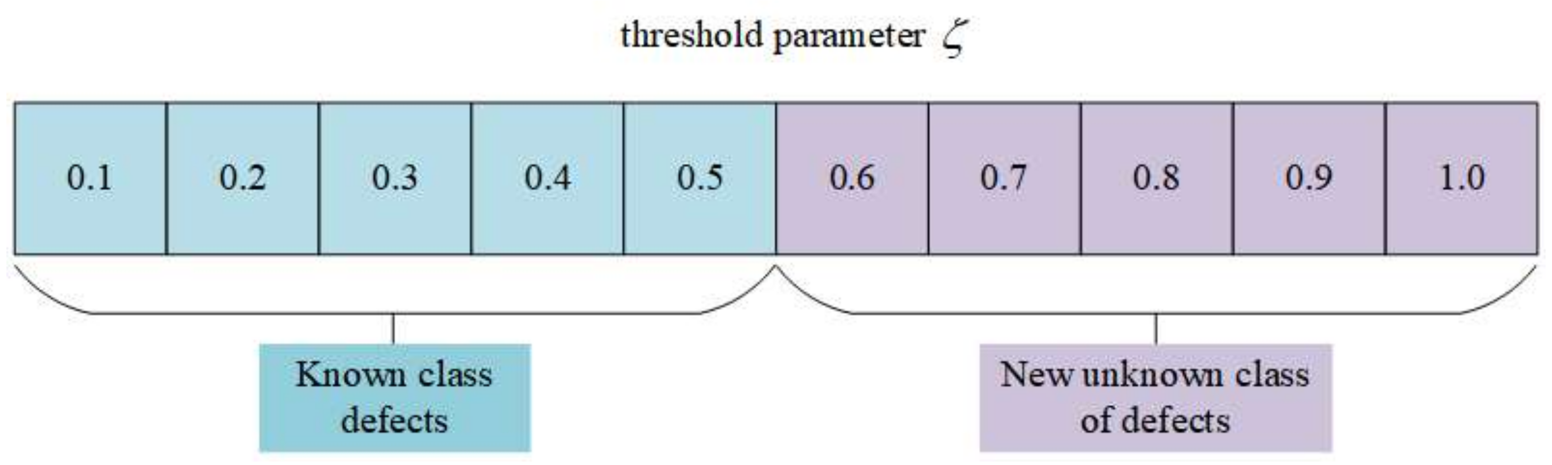
Thresholding parameters for Defect discriminator models
α1The learning rate of domain-invariant feature extractor and Defect discriminator models
α2The learning rate of domain alignment discriminators
Table 2. Detailed description of domain-invariant feature extractor network parameters.
LayerFilter SizePacemakerPaddingOutput Size
Input layer real samples x3 × 128 × 128
Conv2D + BN + LeakyReLU3 × 311128 × 128 × 128
Max pooling layer2 × 22128 × 64 × 64
Conv2D + BN + LeakyReLU3 × 311256 × 64 × 64
Max pooling layer2 × 22256 × 32 × 32
Conv2D + BN + LeakyReLU3 × 311512 × 32 × 32
Max pooling layer2 × 22512 × 16 × 16
Conv2D + BN + LeakyReLU3 × 3111024 × 16 × 16
Global average pooling layer1024 × 1 × 1
FC + ReLU64 × 1 × 1
FC + sigmoid1024 × 1 × 1
Output layer real samples x1024 × 16 × 16
Table 3. Ship painting defect data set setting.
Defect ClassSample ImageSource Domain Sample Data QuantitiesQuantity of Data in the Target
Domain Train Set
Quantity of Data in the Target
Domain Test Set
Label
SaggingCoatings 14 00464 i001300150150SA
Orange skinCoatings 14 00464 i002300150150OS
CrackingCoatings 14 00464 i003300150150CR
BlisteringCoatings 14 00464 i004300150150BL
PinholingCoatings 14 00464 i005300150150PH
DelaminationCoatings 14 00464 i006300150150DF
Table 4. The binary classification confusion matrix.
ClassPredicted Positive ClassPredicted Negative Class
Actual positive classTPFN
Actual negative classFPTN
Table 5. Number of parameters and training time.
ModelParameterTime
TCA182 k1124 s
JDA173 k973 s
DANN227 k572 s
DTL235 k721 s
DCTLN166 k1028 s
TSTAN112 k677 s
IDATLWGAN91 k559 s
Table 6. Comparison of F1-Score, Precision and Recall Rates of Different Transfer Learning Models on Various Defect Categories.
ModelF1-ScorePrecisionRecall
SAOSBLCRPHDF
TCA0.6950.6760.6480.7120.7680.7890.6340.637
JDA0.4870.4970.5730.5390.5720.6250.5190.485
DANN0.8930.7350.8260.8670.8480.8640.7450.812
DTL0.8050.7560.8740.8820.8650.8950.7960.854
DCTLN0.8230.6280.8890.9430.8740.9130.8320.897
TSTAN0.9450.7840.8760.8340.8650.8760.8730.749
IDATLWGAN0.9320.9120.9570.9350.8810.9430.9940.995
Table 7. Detailed description of different migration tasks.
TaskSource Domain→Target DomainSource Domain Dataset Defect ClassTarget Domain Dataset Defect Class
I1A→CSA, OS, CR, PHSA, OS, CR, PH, BL, DF
2C→ASA, OS, CR, PHSA, OS, CR, PH, BL, DF
3B→ESA, OS, CR, PHSA, OS, CR, PH, BL, DF
4E→BSA, OS, CR, PHSA, OS, CR, PH, BL, DF
5C→DSA, OS, CR, PHSA, OS, CR, PH, BL, DF
6D→CSA, OS, CR, PHSA, OS, CR, PH, BL, DF
II7B→ASA, OS, CR, PHSA, OS, CR, PH, BL
8B→ASA, OS, CR, PHSA, OS, CR, PH, DF
9D→ESA, OS, CR, PHSA, OS, CR, PH, BL
10D→ESA, OS, CR, PHSA, OS, CR, PH, DF
11F→BSA, OS, CR, PHSA, OS, CR, PH, BL
12F→BSA, OS, CR, PHSA, OS, CR, PH, DF
Table 8. Detailed description of different ship painting conditions.
Painting ConditionAir Temperature (°C)Relative Humidity (%)
A1550
B1560
C2550
D2560
E3550
F3560
Table 9. Comparison of accuracy (%) of different transfer learning models on different transfer tasks.
Migration ModelTCAJDADANNDTLDCTLNTSTANIDATLWGAN
I137.6538.6451.6357.3467.7884.0890.56
236.2441.1853.1556.6169.4183.2394.74
340.1440.5654.4858.5671.2286.8992.78
438.7837.4449.6753.0064.6784.3391.89
540.8640.3352.2958.3766.8777.8789.77
636.5138.7251.1155.3568.7385.6390.51
Average38.3639.4852.0556.5468.1183.6791.71
II746.5649.4558.7368.1878.0287.7596.03
848.3146.1459.4166.7376.3289.9894.25
945.6848.2163.5963.6874.2186.2393.67
1049.3150.0858.7367.7472.3688.4394.21
1146.5446.3764.6768.2973.0391.7195.57
1244.9546.0859.9665.4379.3793.5892.39
Average46.8947.7260.8566.6875.5589.6194.35
Disclaimer/Publisher’s Note: The statements, opinions and data contained in all publications are solely those of the individual author(s) and contributor(s) and not of MDPI and/or the editor(s). MDPI and/or the editor(s) disclaim responsibility for any injury to people or property resulting from any ideas, methods, instructions or products referred to in the content.

