Investigation of the Influence of Including or Omitting the Oxide Layer on the Result of Identifying the Local Boundary Condition during Water Spray Cooling

Abstract

In the case of products made of steel, the presence of an oxide layer, which is formed during the steel production process as a result of high temperature, has a significant impact on the process of heat removal from the surface of the cooled material. For this reason, it is necessary to take into account the presence of the oxide layer in mathematical and numerical models used to simulate the distribution of the temperature field in cooled steel products. These models are based on the boundary conditions identified for given production conditions. This paper presents a comparison of the results of the identification of the boundary condition during water spray cooling of Armco iron with the use of the inverse solution. Numerical calculations were carried out using two models of heat conduction. In the first model, the presence of an oxide layer with different thermophysical properties than the base material (Armco iron) was taken into account. The second model assumed no oxide layer on the cooled Armco iron surface. It was found that the inverse solution obtained in the case of the heat conduction model taking into account the thickness of the oxide layer is correct in time and as a function of temperature. Thus, the boundary condition model obtained as a function of temperature is universal. However, this model requires an additional layer of oxides with different thermophysical properties than the base material to be included in the finite element model (FEM). Based on the conducted uncertainty tests of the inverse solution, it was found that the results of the determined boundary condition in the absence of the oxide layer on the cooled surface are subject to an error higher than 10% in comparison to the maximum reference value of the heat transfer coefficient.

1. Introduction

Numerical simulations used to model the distribution of the temperature field during the production of steel products allow for reducing production costs, e.g., through energy saving and enable the selection of the parameters of the production process so that the manufactured product has the required properties. In order for the numerical calculations to reflect the actual distribution of the temperature field in the considered object, it is necessary to set the correct boundary conditions for heat transfer. The selection and description of such boundary conditions may be difficult in some cases. This applies in particular to the processes of cooling the surface of hot metals and their alloys using water spray, in which the initial temperature of the cooled object is very high and can reach even 1000 °C. Boundary conditions of heat transfer describing such processes must take into account the specificity of phase transformations of the cooling medium involving different types of boiling. The heat transfer boiling phenomena based on the heat flux data or boiling curve, which describe the variation of the heat flux versus excess temperature, have been extensively described in the literature [1,2,3]. Based on this information, four different regimes of boiling phenomena can be distinguished for the cooling process: (a) film boiling, (b) transition boiling, (c) nucleate boiling, and (d) single-phase free convection.

In the case of cooling objects made of steel, the process of heat removal from the surface of the cooled material is significantly influenced by the presence of an oxide scale, which is formed during steel production processes as a result of high temperature.

The layer of the oxide scale consists of various oxides [4]. The type of oxides, their thickness, and their structure result from the chemical composition of steel, the temperature and time of the heating process, and the surrounding atmosphere during the oxidation process [5,6,7,8]. The oxide layer is a porous layer whose porosity can be higher than 40% [9]. This results in a large dispersion of the thermal conductivity values of the scale reported in the literature [10]. The oxide layer existing on the steel surface limits the heat transfer process between the steel and a coolant. As a result, during the water cooling processes, the existence of the oxide layer strongly influences the Leidenfrost temperature, which is a temperature corresponding to the minimal heat flux. The oxide layer causes the onset of transition boiling which results in intense cooling for a short period of time [11,12,13]. For that reason, it is necessary to consider the presence of the oxide layer in the mathematical and numerical models used to simulate the distribution of the temperature field in the cooled steel products.

This statement was confirmed in [14]. Based on the results of laboratory experiments, including those conducted by other authors, Beigelzimer et al. developed a mathematical model of water-jet cooling of steel plates in the roller-quenching machine, which was then validated for the industrial Thermo-Mechanical Control Process system. To determine the temperature distribution across the thickness of the sheet, a one-dimensional unsteady thermal conductivity equation for a flat, metal plate was solved. The authors present that the obtained results of calculations indicate a good agreement with the measured temperature with the deviation not exceeding 10 °C in the case of including the oxidized layer on the cooled metal surface in the mathematical model of cooling. The omission of the oxide scale in the mathematical model of heat conduction resulted in very rough discrepancies between the calculated and experimental data [14]. The authors emphasize that the oxide layer formed on the cooled product surface is a main factor that introduces uncertainty into the process of the accelerated cooling of metal in production conditions, which changes the real intensity of cooling. The process of cracking and removal of the oxide layer is very difficult to predict because it is a random event.

The boundary conditions during accelerated cooling are determined by using several mathematical models that employ the inverse solution to the heat conduction problem.

Some of them are used to describe the heat transfer during the spray cooling process of different metals or alloys [15,16,17,18]. Using such models allows the heat transfer coefficient, which is correlated with the temperature of the cooled metal surface, to be obtained. However, these models do not take into account the thickness and properties of the oxide scale on the surface of the cooled metal. As was mentioned before, using data obtained from models in which the oxide layer is not included to simulate temperature distribution inside the cooled metal may lead to inaccurate results. It can be assumed that the error results from the omission of the oxide layer will be small in case of its thin thickness (below 10 µm) or rapid descaling under the influence of water fed under high pressure in the case of low alloy steels for which the oxide layer is not stable enough to withstand spray cooling [10]. In the case of thin homogeneous and adhesive oxide layers, the thickness of the scale and the descaling during spray cooling influence the local heat transfer causing inhomogeneous cooling.

There are only a few models that allow the determination of the boundary conditions during spray cooling for steel covered with an oxide layer. One of them introduced the concept of an effective heat transfer coefficient [13,19,20,21,22]. The insulating effect of scale is described mathematically using the analogy of heat transfer through a wall with insulation. The oxide layer is treated as an isolation layer with known heat resistance that is described by its thickness and thermal properties (thermal conductivity). The temperature of the oxide-free steel surface is obtained from the numerical simulation of the cooling process. Based on this date, the heat transfer coefficient (HTC) on the oxide-free surface is calculated from Newton’s Law. The effective heat transfer coefficient on the scale surface is obtained by reducing the HTC value by the thermal resistance of the oxide layer [13,19,20,23].

Such a definition of the heat transfer coefficient makes it possible to omit the modeling of heat transfer through the scale layer and the phenomena associated with its formation. It simplifies the numerical simulation of the cooling process. The heat transfer coefficient needs to be calculated from the numerical model does not consider the oxide layer when the surface temperature of the non-oxide metal is known. For this purpose, the relations developed on the basis of experimental investigation described in publications can be used [15,24,25].

Another model used for the identification of the boundary conditions was presented in [26]. The existence of the oxide layer on the surface of a steel plate was considered in the FEM of conduction. This model requires the introduction of scale modeling elements near the surface.

For that reason, in the FEM model, two layers made of different materials with different thermophysical properties were assumed. The first layer was steel and the second was the oxide layer. The density of the oxide layer is lower than that of steel; therefore, during the oxidation process, the thickness of the oxide layer increases, increasing the initial thickness of the material. This phenomenon was taken into account by increasing the size of the elements modelling the heat flow through the oxide layer while reducing the thickness of the steel layer. The thickness of the oxide layer was calculated based on the time it was formed. The results of the calculations were consistent with the results of physical measurements. It should be emphasized that the temperatures derived from the FEM model presented in [26] are the actual temperatures of the surface on which the oxide layer is located.

In both types of numerical models where the presence of the oxide layer is considered, the constant thickness of the scale during the entire cooling period is assumed. This assumption is not correct because during the cooling the scale may crack and be removed from the cooled surface. However, this process is difficult to predict and the entering of a constant scale thickness in the numerical model will affect the result of inverse calculations in this case. The inverse problems are classified as ill posed, which means that the errors in the input data are transferred with increasing amplitude to the calculation results. The main sources of the error connected with the input data are temperature measurement errors, the uncertainty to the thermophysical properties of the steel and oxide layer, as well as the method of the boundary condition approximation. For that reason, solving the inverse heat transfer problems is considered challenging [27].

The aim of this paper is to compare the results of the identified boundary condition for the Armco iron cooling process using the inverse solution of the heat conduction equation. Numerical calculations were carried out using two models of heat conduction. In the first model, the presence of an oxide layer with different thermophysical properties than the base material (Armco iron) was taken into account. The second model assumed no scale layer on the cooled surface of the Armco iron. The research results presented in the literature so far make it possible to determine the impact of the existence of the oxide layer (its thickness, thermal conductivity) on the HTC and on the development of the boiling process during water spray cooling, but do not answer the question about the error in determining HTC when using a specific model employ to determine boundary condition. The authors of this paper attempted to answer this question using one of the models (including three-dimensional heat conduction). It is worth emphasizing that the inverse numerical model used by the authors allows the analysis of the local changes in the HTC values.

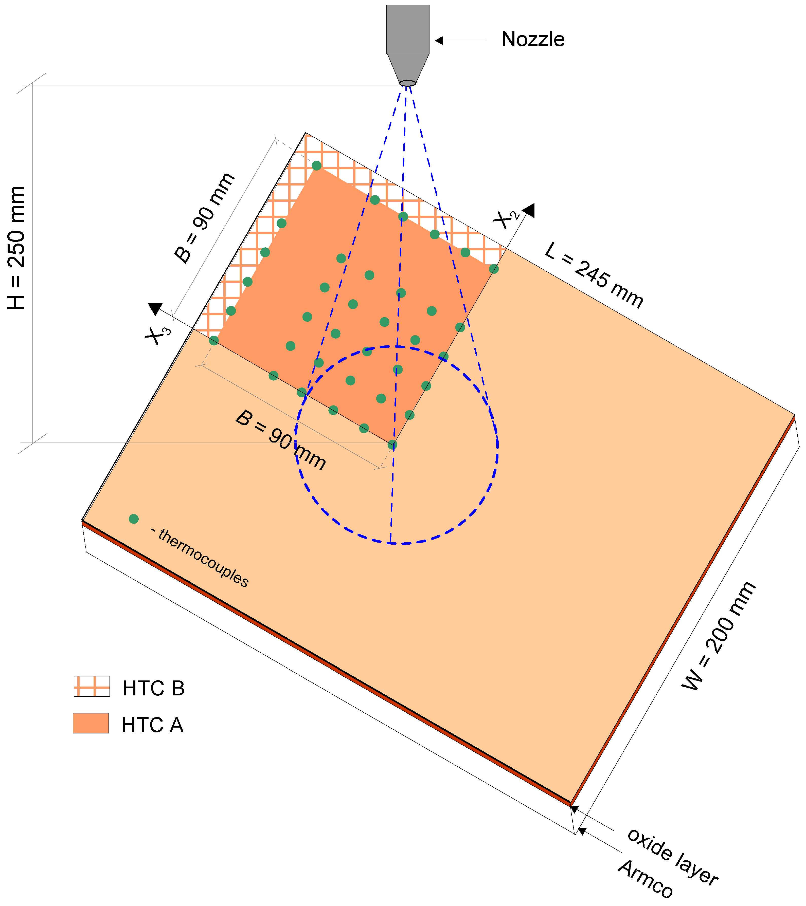
2. Experimental Setup

To compare the results of the boundary condition identification by two numerical models the experimental investigations were carried out. The investigation included five cycles of heating and cooling plate made of Armco iron. The plate dimensions were 245 × 200 × 8 mm (long × wide × thickness). In each test, the plate was heated to 700 °C and cooled to 50 °C with a water-spray nozzle. To heat the plate an electric furnace was used. The process was carried out in an air atmosphere until the temperature of the plate became uniform. The transport time of the plate from the furnace to the cooling chamber was 5 s. The same plate was used for each heating and cooling cycle. During the heating process, an oxide layer was created on the plate surface. The thickness of the oxidized layer was measured as described in [26]. During the cooling process, the upper surface of the plate was cooled with the spray nozzle. The heat transfer process at the bottom surface was by natural convection and radiation. For the cooling tests, a 45° full-cone nozzle was used. The spray nozzle was located 250 mm above the plate, approximately in the center of the plate Figure 1. The water spray pressure was 0.1 MPa and the temperature of the cooling water was 17.5 °C. Based on the measurements of water spray distribution described in [15], a hydraulic characteristic of the nozzle was developed. The function described water spray distribution from the 45° full-cone nozzle that was presented in [26]. The inverse calculation allowing determination of the change in the heat transfer coefficient (HTC) and heat flux (HF) was carried out for only one-quarter of the water flow zone because of the symmetry of the cooling process. The area on which the HTC and HF were identified was a square with side B equaling ninety millimeters, Figure 1.

To measure the temperature, thirty-six K-type thermocouples with 80 µm diameter wires protected by a 500 µm diameter sheath were used, as shown in Figure 1. Thermocouples were placed two millimeters below the cooled surface. The data acquisition system, which was used to record the temperature measurements, was equipped with a noise reduction filter. The maximum error of the measured temperature was about ±0.6% [26].

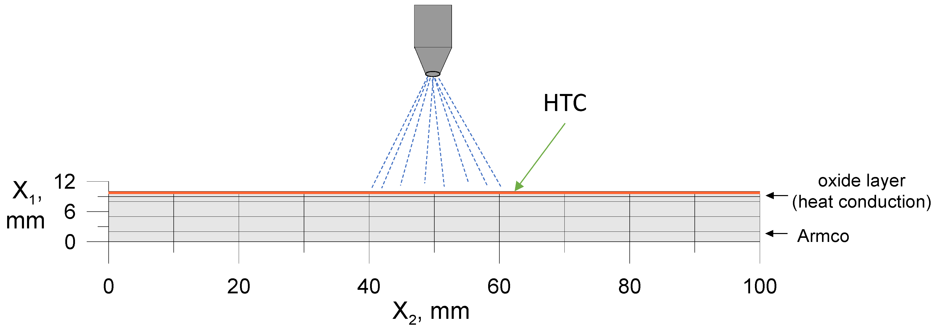
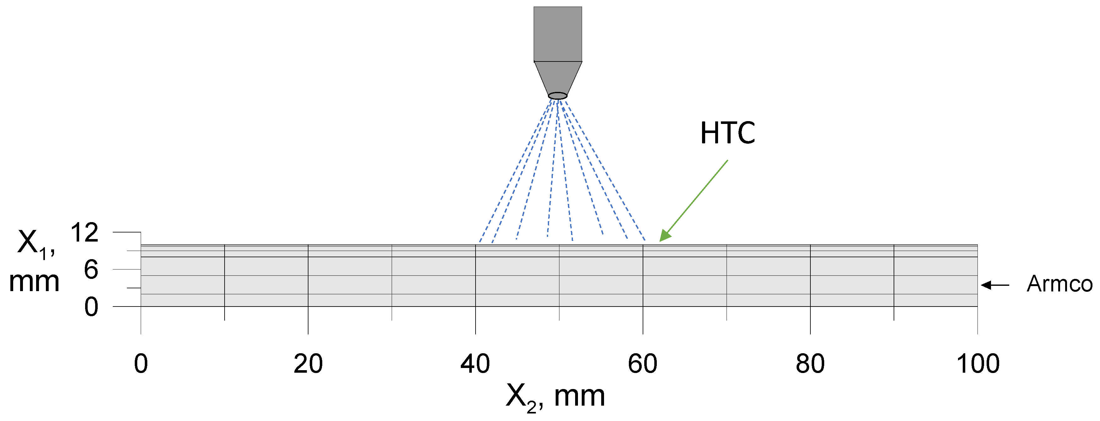
3. Model of Heat Conduction in a Plate

The plate temperature calculations were performed by solving the Fourier–Kirchhoff equation by using the finite element method [26].

A detailed description of the heat conduction numerical model was presented in [28]. In order to compare the influence of using a numerical model of heat conduction with or without an oxide layer on the identified boundary conditions, two calculation variants were carried out. In the first variant of the calculation, a heat conduction model called HC-Model 1 was used. In this model, the presence of the oxide layer was included. The base layer was Armco iron, and the second layer was the oxide layer (Figure 2). In the calculation, the increase in the thickness of the oxide layer was included by increasing the thickness of the element adjacent to the surface [26]. For the thickness of the 0.018 mm oxide layer, it was 0.005 mm, and for the thickness of 0.035 mm, it was 0.011 mm. Figure 2 shows the division of the Armco iron plate into elements along its thickness with marked near-surface elements corresponding to the oxide layer. Based on the data presented by Mu Li et al., the thermal properties of the oxide layer were assumed as follows: thermal conductivity 2.3 W/(m·K), and the specific heat was 870 J/(kg·K) [29]. The increase in the oxide layer thickness during the oxidation process was calculated from the equation obtained on the basis of laboratory tests [26]. Thermal properties of the Armco iron were assumed as temperature dependent [30]. The surface temperature obtained from the numerical solution in the case of using the heat conduction model HC-Model 1 is the physical temperature on the surface of the oxide layer.

The second variant of the calculation was performed by using a heat conduction model without an oxide layer. This model was named HC-Model 2. The division of the cooled Armco iron plate along its thickness is presented in Figure 3. The emissivity of the plate surface was assumed to be the same as the emissivity of the oxide layer. The surface temperature values obtained from the numerical solution based on the calculation carried out by using HC-Model 2 did not include the amount of heat conducted through a layer with different thermal properties than Armco iron.

The spray nozzle was placed above the center of the plate, which resulted in the symmetry of the water flow. For this reason, the calculations were performed for the marked area 100 mm by 100 mm (Figure 1). On the two plans of symmetry zero HF values were assumed ${\dot{q}}_1$ and ${\dot{q}}_2$ (Figure 1). On the bottom surface of the plate the boundary conditions ${\dot{q}}_{bottom}$ resulting from the plate cooling in the cooling chamber was specified the same as described in [26].

The convective heat losses when the plate was transported to the cooling chamber were calculated based on the Nusselt number (Nu) [26]. The water-cooled upper surface of the plate was divided into two areas (Figure 1). The HTC A area corresponds to the part of the plate where the thermocouples were placed. This was the HF determination domain. The remainder of one-quarter of a plate was designated as the HTC B domain. The equations describing the boundary conditions in these two domains can be found in [26].

The unknown HTC coefficients present in the equations that defining the boundary conditions at the HTC A domain were determined from the inverse solution to heat conduction problem of the plate cooling [26].

Accuracy of the Finite Element Solver

To compute temperature of the plate, the finite element solver developed by Malinowski et al. [28] was used. The accuracy of the temperature field solution for HC-Model 2 without oxide layer was presented in [15]. The obtained results of calculations gave a maximum temperature error ∆T_max = 2.3 °C. In case of HC-Model 1 with the oxide layer, additional tests were performed. The procedure of testing the accuracy of the heat conduction numerical model HC-Model 1 (with the oxide layer) was the same as the one presented in [15]. First, the finite element solver of HC-Model 1 was tested on J. Fourier one-dimensional solution for the heat conduction problem [31]. The test was performed for the steel plate and the HTC = 20 kW/(m²·K). The thermophysical properties of steel were assumed as constant. The FEM reference model (Re-M) with 13 linear elements in the x₁ direction (along the thickness of the plate) and time increment ∆τ = 0.1 s gave the average temperature error (ATE) of 0.2 °C compared to the analytical model (An-M). To reduce the time of numerical calculations, two other models were tested in which the number of elements were reduced compared to the Re-M. The M-1 model with five linear elements in the x₁ direction gave the ATE = 1.44 °C to the analytical solution. In model M-2, seven linear elements in the thickness of the plate reduced the ATE to 0.17 °C for the time increment of ∆τ = 0.05 s and gave the same accuracy as the Re-M for ∆τ = 0.1 s. Thus, for modelling the Armco iron plate cooling, seven linear elements in the plate thickness can be employed. The temperature field of Armco iron during water spray cooling is different from one-dimensional heat conduction [26]. Therefore, further FEM solver tests were performed to determine the accuracy of the numerical calculations in the case of non-uniform temperature field caused by the water spray cooling. For the FEM solver tests and for the determination of the uncertainty of the inverse solutions, the HF ${\dot{q}}_{upper}$ at the upper surface of the plate was assumed as a test function. The adopted test function allows model the water spray cooling process [26].

The $h_{upper}$ function defining the HTC for modeling the water spray cooling was developed based on the real experimental data obtained from the Armco steel spray cooling process. The $h_{upper}$ was approximated by the product of functions [26]:

$$h_{upper}={\dot{w}\left(x_2,x_3,H,p\right)}^{0.43}D\left(T_S\right)$$

(1)

The method of constructing the approximation function D was described in [15]. The function D in Equation (1) is a thermal characteristic of the coolant. The parameters of the reference function D were developed for the Armco iron plate cooling with the full cone nozzle with a spray angle of 45°, for a water pressure of p = 0.1 MPa, and for the nozzle located 250 mm above the plate. The water flux distribution was described by two functions that approximates water flux distribution from the stagnation point to infinity. The equations and parameters described by these two functions were given in [15]. At the side surfaces of the plate, vertical to domain B, the following boundary condition was assumed [26]:

$${\dot{q}}_{side}=3.31·{10}^6\frac{{\dot{w}}^{0.616}}{t_s^{2.445}} \left(t_s-t_w\right)$$

(2)

This boundary condition describing the dependency of the HF on the water flux and surface temperature was developed by Hodson [32]. For the FEM solver tests, the water flux rate $\dot{w}$ was calculated according to the equation given in [15], for the water pressure p = 0.1 MPa and the distance between the spray nozzle and the cooled surface H = 250 mm.

The Armco iron plate temperature was calculated using the FEM Re-M model. The boundary conditions defined by ${\dot{q}}_1$, ${\dot{q}}_2$, ${\dot{q}}_{side}$, ${\dot{q}}_{bottom}$ ${\dot{q}}_{upper}$ were specified at the plate surfaces. The thickness of the oxide layer g_z = 0.028 mm was assumed in the calculation. The plate temperature at the thermocouple locations was computed and compared to that obtained from the M-1, M-2, and M-2a models. The results of the simulation of the plate temperature with the reduced models are summarized in

Table 1. Accuracy of the finite element models in forward simulation of the Armco iron plate cooling.

Parameter		Heat Conduction Model (HC-Model 1)
		Re-M	M-1	M-2	M-2a
No. of elements in x1 direction		13	5	7	7
No. of elements in x2 direction		23	10	10	10
No. of elements in x3 direction		23	10	10	10
Time increments, s	∆τ	0.1	0.1	0.05	0.1
Error to Re-M, °C	ATE	0	0.91	1.16	0.92
Error to An-M, °C	ATE	0.2	1.44	0.17	0.80

. In the case of the realistic cooling conditions, the M-1 model and M-2a model gave the same accuracy as the Re-M model for time increment ∆τ = 0.1 s. Decreasing the time increment to ∆τ = 0.05 s, in the case of model M-2a, did not improve the accuracy of the heat conduction equation solution. For that reason, in the case of the HC-Model, similar to HC-Model 2, for the inverse solution, model M-2a was chosen.

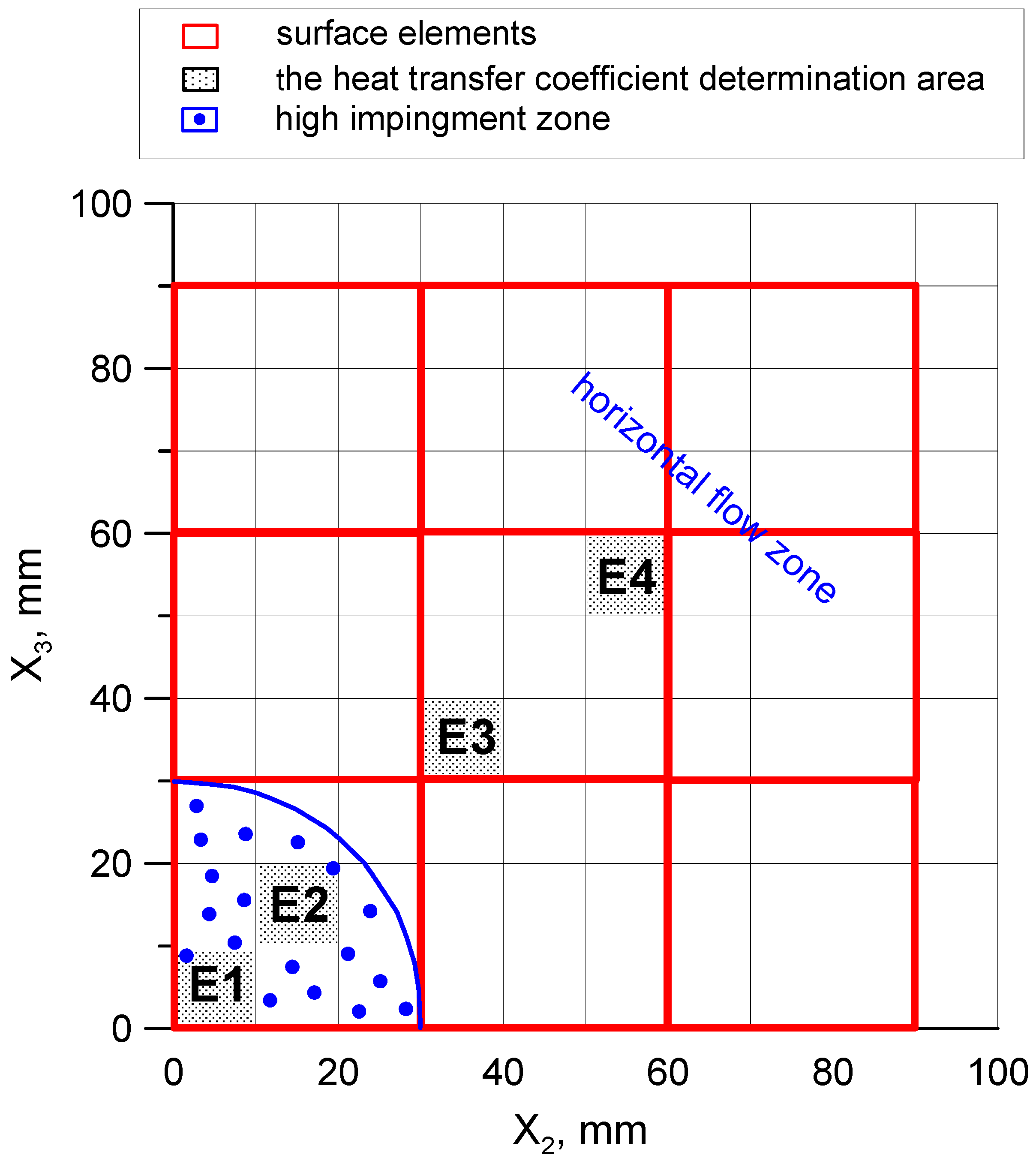
4. The Inverse Problem Formulation

The HF and HTC at the upper surface of the plate for water cooling were identified by using the method developed by Malinowski et al. [33]. To obtain the inverse solutions to the HTC distribution over the plate surface, the objective function presented by Hadała et al. was used during the optimization procedure [34].

The HTC distribution over HTC A was approximated by surface elements with parabolic shape functions N_i. The division of the HTC A area into nine surface elements is shown in Figure 4.

The HTC distribution over the HTC A area is determined from the minimum condition of the objective function. The solution procedure for this problem is presented in [34].

Uncertainty of the Inverse Solution

To determine the accuracy of the inverse solution to the HTC distribution in space and time, the uncertainty tests were performed. In the uncertainty tests, the boundary condition described by Equation (1) was searched. The Armco iron plate temperature was simulated using the FEM reference model (Re-M) with 13 linear elements in the x₁ direction and 23 linear elements in the x₂ and x₃ directions, respectively. The boundary conditions defined by: ${\dot{q}}_1$, ${\dot{q}}_2$, ${\dot{q}}_{side}$ ${\dot{q}}_{bottom}$ were specified at the plate surfaces. At the upper surface of the plate, the HF was described by Equation (1). The parameters defining the function D, were obtained from a physical cooling test of the Armco iron plate at pressure p = 0.1 MPa and the distance to the plate H = 250 mm. In the calculation, the thickness of scale layer g_z = 0.028 mm was assumed. Using the reference model (Re-M), the plate temperature at 36 points shown in Figure 1 was recorded as the simulated temperature sensor indications. For the inverse solution, the FEM model with 7 linear elements in the x₁ direction and 10 linear elements in the x₂ and x₃ directions was used. The time increment ∆τ was 0.1 s. The calculations were performed for two variants of the heat conduction model with (HC-Model 1) and without (HC-Model 2) the oxide layer. In both cases, the results of the calculations were compared to the specified boundary condition denoted as ETF at selected areas marked E₁–E₄, which are shown in Figure 4. The E₁ area is located in the stagnation zone, and the E₂ area is placed in the high impingement zone. The areas marked as E₃ and E₄ are placed in the horizontal flow zone. For the inverse solution, the time of cooling was divided into 24 periods. It gave 2920 $h_{HTC A}$ as the coefficient to be determined from the minimum condition of the objective function.

The test performed for the HC-Model 1 made it possible to identify the deviation of the inverse solution from a real boundary condition resulting mainly from the temperature measurement errors and the limited number of temperature sensors. The test carried out for the HC-model 2 allowed the identification of the errors resulting from the omission of the oxide layer on the Armco iron surface.

To determine the error between the reference model (Re-M) and the numerical reduce model (M-2a) that was used in the inverse calculations, the average temperature distance (ATD) between these two models was computed according to the following equation [15]:

$$\mathrm{A}\mathrm{T}\mathrm{D}=\sqrt{\frac{1}{NT NP}\sum _{n=1}^{NT}\sum _{m=1}^{NP}{\left[\frac{{Te}_n^m-{T\left(h_i\right)}_n^m}{\sqrt{1+{\left(\frac{∆{Te}_n^m}{∆\tau }\right)}^2}}\right]}^2}$$

(3)

In Equation (3), ${Te}_n^m$ is a sample temperature obtained from the Re-M at the sensor n and at the time ${\tau }_m$. The term in brackets defines the temperature distance ∆T_n between two curves T (τ) and T_e (τ) always normal to the T_e (τ) curve [34].

For HC-Model 1 the inverse solution converged to the average distance ATD = 0.60 °C with the maximum distance between the temperature curves ∆T_n = 2.1 °C. Omission of the oxide layer in the numerical model of heat conduction (HC-Model 2) did not significantly change the values of these two parameters. The ATD for this variant of calculation was 0.61 °C and the maximum distance between the temperature curves was 2.3 °C. In Figure 5 the plate surface temperatures at areas E₁–E₄ are compared to the reference solution. The plate surface temperature obtained from the inverse solution for both variants of calculations is almost identical to the reference model in which the oxide layer was included. That allow conclude that both models can be used to simulate the temperature changes in the cooled material.

In Figure 6, the obtained distribution of the HTC at E1, E2 and E3 areas is shown. The HTC distribution is very close to the search boundary condition (ETF) for both heat conduction models. However, in the case of employing to the inverse calculations the HC-Model 2 in which the oxide layer was not included, the HTC values differ much more from the reference boundary condition than in the case of using the HC-Model 1 where the oxide layer was considered. The error to the maximum value of specified ETF boundary condition for each of these three areas is over 10% when using the HC-Model 2 (

Table 2. Accuracy of the 3D inverse solution utilizing the M2a model to the specified boundary condition ETF.

Parameter		Model with Oxide Layer (HC-Model 1)				Model without Oxide Layer (HC-Model 2)
Element		E1	E2	E3	E4	E1	E2	E3	E4
Error to the ETF maximum		−1.6%	+2.0%	+1.0%	−23.3%	+13.3%	+15.5%	+10.1%	−12.4%
ATD	°C	0.60				0.61
∆Tn	°C	2.1				2.3

). The use of the HC-Model 1 in this case allows significantly reduce the error in identifying boundary condition.

5. Results of the Identification of the Heat Transfer Boundary Conditions

The temperature variations obtained from the inverse solution by using the heat conduction model with (HC-Model 1) and without the oxide layer (HC-Model 2) at the selected points for the thickness of the oxide layer 0.018 mm were compared to the measured temperatures in Figure 7. The calculated temperatures are almost the same as those measured in both variants of calculations. The accuracy of the inverse solution described by ATD is presented in

Table 3. Accuracy of the inverse solution.

Thickness of the Oxide Layer, mm	Model Number	ATD, °C
0.018	HC-Model 1	0.42
	HC-Model 2	0.35
0.035	HC-Model 1	0.42
	HC-Model 2	0.34

. In case of employing to the inverse calculations heat conduction model included oxide layer (HC-Model 1) the ATD did not exceed 0.42 °C. The accuracy of the temperature calculations obtained from the inverse solution where no oxide layer was considered (HC-Model 2) was slightly better and the ATD did not exceed 0.35 °C. Based on the values of the ATD, it can be stated that both models of heat conduction used for the inverse calculation give the correct solution. This is so in the case of temperature variations. However, in the case of boundary conditions described by thee HF or HTC, significant differences are observed (Figure 8, Figure 9, Figure 10 and Figure 11).

A comparison of the HF variations presents in Figure 8 and Figure 9 revealed differences between the course of the HF curves in the transition and nucleate boiling regimes. The choice of HC-Model 2 for the inverse calculation resulted in shifting the HF to higher temperatures in the range of transition and nucleate boiling. The maximum HF in the areas E₁ is the same regardless of the heat conduction model employed for the inverse calculations for both oxide layer thicknesses. However, for the areas placed in the high impingement (E₂) and horizontal flow zones (E₃), higher values of the maximum HF were obtained for the inverse solution employing HC-Model 2. The difference between the maximum HF calculated from the inverse solution using HC-Model 1 and HC-Model 2 for the E₂ area is smaller for lower oxide layer thickness. The maximum HF calculated from the inverse solution using HC-Model 2 is higher than the one obtained from HC-Model 1 by 0.3% for the oxide layer thickness of 0.018 mm and for the thickness of 0.035 mm by 2.2%. In the horizontal flow zone for the E₃ area, the difference between the maximum HF is independent of the oxide layer thickness and equaled 11.4%.

The comparison of the identified HTC obtained from the inverse calculation by using two heat conduction models for considered thicknesses of the oxide layer is presented in Figure 10 and Figure 11. The comparison shows the shift of the maximum HTC to higher temperatures for areas placed in the high impingement zone. For the oxide layer thickness of 0.018 mm, the shift is 15 °C (Figure 10) and for the thickness of 0.035 mm, it is 24 °C (Figure 11). Inverse calculations performed using HC-Model 2, which does not include the oxide layer, result in a decrease in the maximum HTC and a greater actual thickness of the oxide layer. For the oxide layer thickness of 0.018 mm, the maximum HTC obtained by using HC-Model 2 is lower than the one obtained with HC-Model 1 by 11.5% in the E₁ and E₂ areas (Figure 10). In the case of the oxide layer thickness of 0.035 mm, the maximum HTC decreases by 19% in the E₁ area and by 16% in the E₂ area (Figure 11).

This relation indicates that in the case of identification of the HTC by using the inverse heat transfer solution, using the heat conduction model does not include the presence of the oxide layer, and the obtained results may underestimate the HTC values, especially when the actual thickness of the oxide layer is high. It can be concluded that in the case of identification of the boundary condition below the Leidenfrost temperature, the choice of the FEM heat conduction model is important. The transfer of heat energy in transition and nucleate boiling regimes is very intense; therefore, the influence of the thickness of the oxide layer with a small thickness and much lower thermophysical properties in relation to steel cannot be ignored.

For both heat conduction models, for the examined thickness of the oxide layer, an identical model of boundary condition in the range of film boiling regime was obtained (Figure 8, Figure 9, Figure 10 and Figure 11). Such results might be caused by the low heat transfer resulting in heat transfer mechanisms that take place on the metal-cooled surface during film boiling (heat conduction through the vapor layer and radiation from the metal surface to the liquid layer).

6. Conclusions

Identification of the boundary conditions during the process of cooling a hot metal surface with water spray is a difficult problem especially when the metal surface is covered with an oxide layer. The inverse solution to the heat transfer problem which is commonly used to identify the boundary conditions in such cases is very sensitive to the errors in the input data. Also, the mathematical model of heat conduction used in the inverse method has an influence on the obtained solution. Not including the oxide layer in this model may lead to incorrect results in the identification. In this paper, two FEM models of heat conduction were compared in order to estimate the error of not including the presence of the oxide layer in the heat conduction model employed to the inverse solution.

The results obtained allowed us to draw the following conclusions:

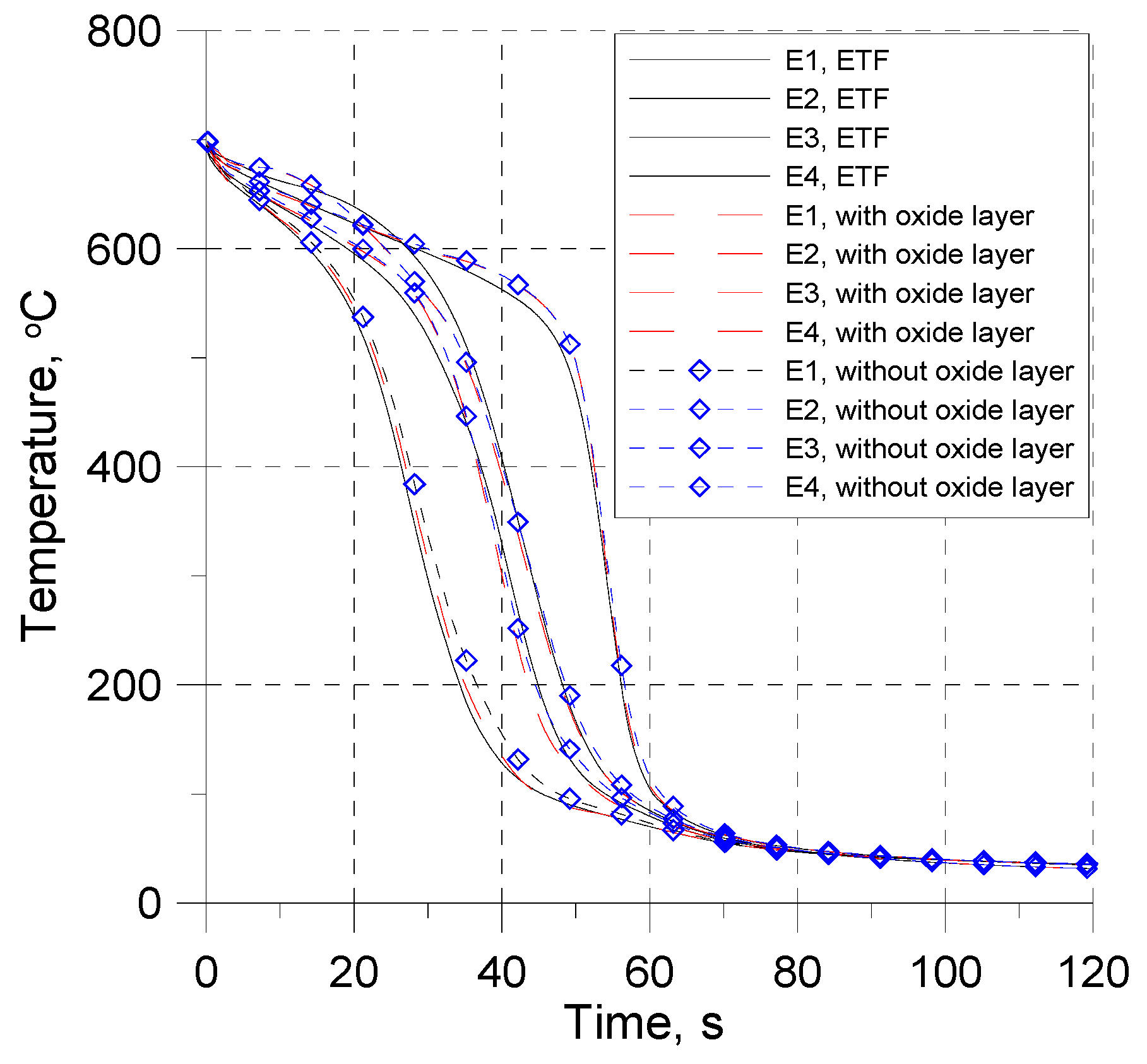
• Mathematical models of heat conduction that do not consider the presence of oxide ignore the different heat capacity and thermal conductivity of the oxide layer in relation to the metal. The heat capacity of the scale and its conductivity are much lower than that of steel which significantly affects the heat transfer process that takes place on the cooled surface.
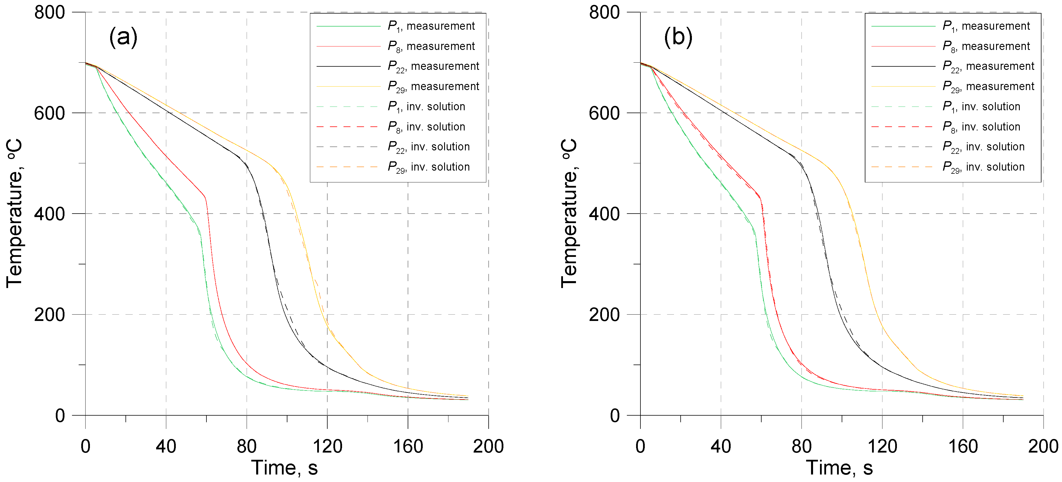
• The inverse solution obtained in the case of using the conduction model, which takes into account the thickness of the oxide layer, is correct in time and as a function of temperature. The error of the numerical calculation is 0.6 °C, which indicates a great accuracy of the inverse solution. Thus, the model of the boundary condition obtained as a function of temperature is universal.
• For a thin oxide layer, the FEM model of heat conduction can be simplified, so there is no need to consider the presence of the oxide layer, at least for the temperature field calculation.
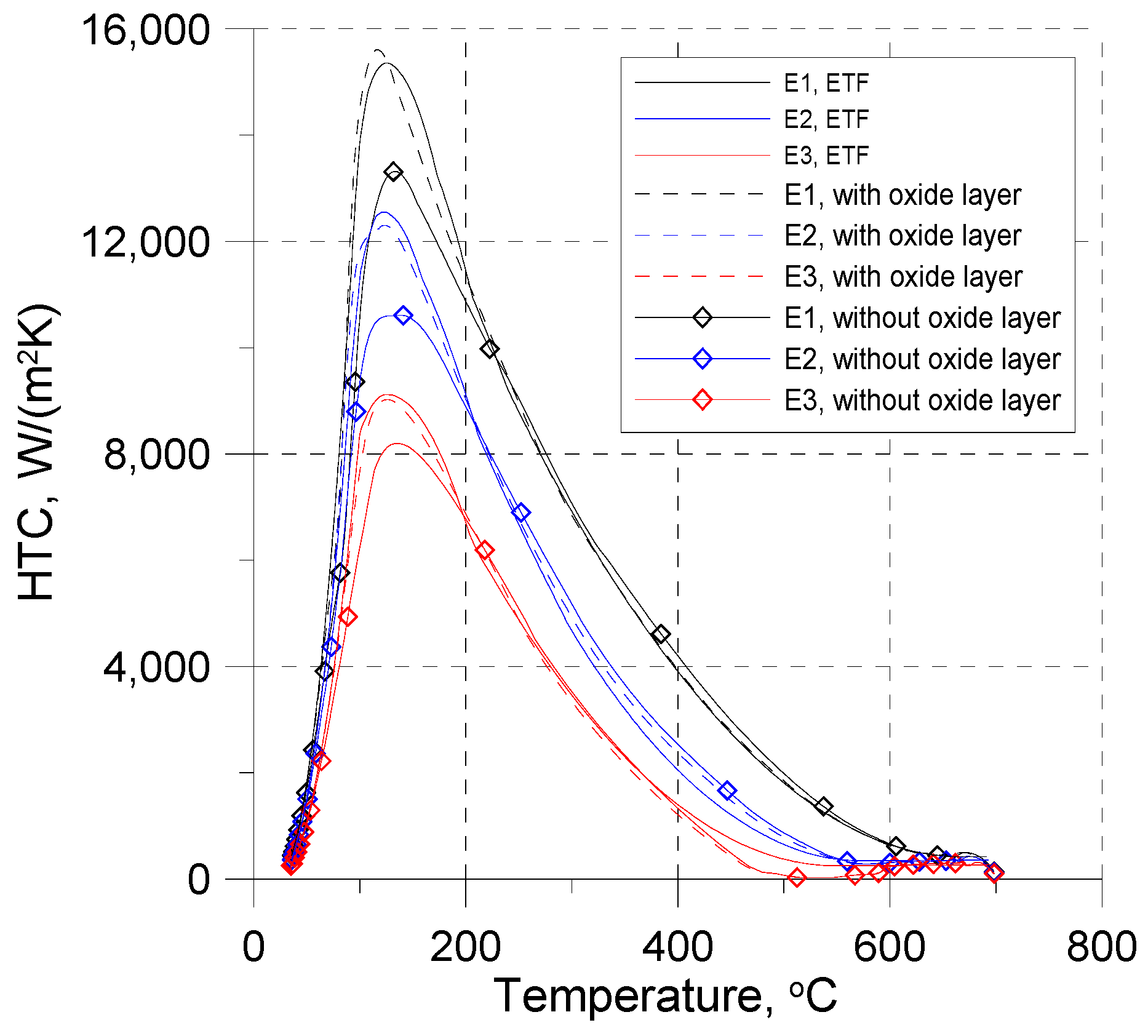
• For the boundary condition determination, it is better to use an accurate model, taking into account the presence of the oxide layer on the cooled surface, because the results of the determined boundary condition are subject to an error of at least an order of magnitude smaller than when using a simplified model of heat conduction for calculations.

Further research will focus on the investigation of the impact of different coatings on the intensity of heat collection and on developing a model of the heat transfer boundary condition for water spray cooling of oxidized surfaces.

References

1. Çengel, Y.A. Heat and Mass Transfer: A Practical Approach, 3rd ed.; McGraw-Hill: New York, NY, USA, 2007. [Google Scholar]
2. Holman, J.P. Heat Transfer, 10th ed.; McGraw-Hill: New York, NY, USA, 2010. [Google Scholar]
3. Mudawar, I.; Valentine, W.S. Determination of the local quench curve for spray-cooled metallic surfaces. J. Heat Treat. 1989, 7, 107–121. [Google Scholar] [CrossRef]
4. Horsky, J.; Hrabovsky, J.; Raudensky, M. Impact of the scale on spray cooling intensity. In Proceedings of the 10th International Conference on Heat Transfer, Fluid Mechanics and Thermodynamics (HEFAT 2014), Orlando, FL, USA, 14–16 July 2014; pp. 1480–1485. [Google Scholar]
5. Slowik, J.; Borchardt, G.; Köler Ch Jeschar, R.; Scholtz, R. Influence of oxide scales on heat transfer in secondary zones cooling in the continues casting process, part 2: Determination of material properties of oxide scales on steel under spray-water cooling conditions. Steel Res. 1990, 61, 302–311. [Google Scholar] [CrossRef]
6. Wendelstorf, J.; Spitzer, K.H.; Wendelstorf, R. Spray water cooling heat transfer at high temperatures and liquid mass fluxes. Int. J. Heat Mass Transf. 2008, 51, 4902–4910. [Google Scholar] [CrossRef]
7. Burakowski, T. Własności promienne stali chromowych. Metalozn. i Obróbka Ciepl. 1973, 3, 31–40. [Google Scholar]
8. Béranger, G.; Henry, G.; Sanz, G. (Eds.) The Book of SteelScientific; Intercept Limited: Andover Hampshire, UK, 1996. [Google Scholar]
9. Resl, O.; Chabicovský, M.; Votavov’a, H. Study of thermal conductivity of the porous oxide layer. In Proceedings of the 25th International Conference Engineering Mechanics, Svratka, Czech Republic, 13–16 May 2019; pp. 315–318. Available online: http://www.engmech.cz/im/proceedings/show_p/2019/315 (accessed on 3 July 2024).
10. Takeda, M.; Onishi, T.; Nakakubo, S.; Fujimoto, S. Physical properties of iron-oxide scales on si-containing steels at high temperature. Mater. Trans. 2009, 50, 2242–2246. [Google Scholar] [CrossRef]
11. Chabičovský, M.; Hnizdil, M.; Tseng, A.A.; Raudenský, M. Effects of oxide layer on Leidenfrost temperature during spray cooling of steel at high temperatures. Int. J. Heat Mass Transf. 2015, 88, 236–246. [Google Scholar] [CrossRef]
12. Resl, O.; Chabičovský, M.; Hnízdil, M.; Kotrbáček, P.; Raudenský, M. Influence of Porous Oxide Layer on Water Spray Cooling. In Proceedings of the 9th International Conference on Fluid Flow, Heat and Mass Transfer (FFHMT’22), Niagara Falls, ON, Canada, 8–10 June 2022; p. 125. [Google Scholar] [CrossRef]
13. Wendelstorf, R.; Spitzer, K.-H.; Wendelstorf, J. Effect of oxide layer on spray water cooling heat transfer at high surface temperatures. Int. J. Heat Mass Transf. 2008, 51, 4892–4901. [Google Scholar] [CrossRef]
14. Beygelzimer, E.; Beygelzimer, Y. Validation of the Cooling Model for TMCP Processing of Steel Sheets with Oxide Scale Using Industrial Experiment Data. J. Manuf. Mater. Process. 2022, 6, 78. [Google Scholar] [CrossRef]
15. Cebo-Rudnicka, A.; Malinowski, Z. Identification of heat flux and heat transfer coefficient during water spray cooling of horizontal copper plate. Int. J. Therm. Sci. 2019, 145, 106038. [Google Scholar] [CrossRef]
16. Sabariman, E. Specht, Characterization of the boiling width on metal quenching with spray cooling. Exp. Heat Transf. 2018, 31, 391–404. [Google Scholar] [CrossRef]
17. Singh, A.P.; Prasad, A.; Prakash, K.; Sengupta, D.; Murty, G.M.D.; Jha, S. Influence of thermomechanical processing and accelerated cooling on microstructures and mechanical properties of plain carbon and microalloyed steels. Mater. Sci. Technol. 1999, 15, 121–126. [Google Scholar] [CrossRef]
18. Liu, W.-W.; Li, H.-J.; Wang, Z.-D.; Wang, G.-D. Mathematical model for cooling process and its self-learning applied in hot rolling mill. J. Shanghai Univ. 2011, 15, 548–552. [Google Scholar] [CrossRef]
19. Kohler, C.; Jeschars, R.; Scholz, R.; Slowik, J.; Borchardt, G. Influence of oxide scales on heat transfer in secondary cooling zones in the continuous casting process, part 1: Heat transfer through hot-oxidized steel surfaces cooled by spray-water. Steel Res. 1990, 61, 295–301. [Google Scholar] [CrossRef]
20. Raudensky, M.; Chabicovsky, M.; Hrabovsky, J. Impact of oxide scale on heat treatment of steels. In Proceedings of the METAL 2014 23rd International Conference on Metallurgy and Materials, Conference Proceedings, Ostrava, Czech Republic, 21–23 May 2014; Tanger Ltd.: Greensboro, NC, USA, 2014; pp. 1–6, ISBN 978-80-87294-52-9. [Google Scholar]
21. Mraz, K.; Bohacek, J.; Resl, O.; Chabicovsky, M.; Karimi-Sibaki, E. Thermal conductivity of porous oxide layer: A numerical model based on CT data. Mater. Today Commun. 2021, 28, 102705. [Google Scholar] [CrossRef]
22. Fukuda, H.; Nakata, N.; Kijima, H.; Kuroki, T.; Fujibayashi, A.; Takata, Y.; Hidaka, S. Effects of Surface conditions on spray cooling characteristics. ISIJ Int. 2016, 56, 628–636. [Google Scholar] [CrossRef]
23. Viscorova, R.; Scholz, R.; Spitzer, K.-H.; Wendelstorf, J. Spray water cooling heat transfer under oxide scale formation conditions. Adv. Comput. Methods Heat Transf. IX 2006, 53, 163–172. [Google Scholar] [CrossRef]
24. Liang, G.; Mudawar, I. Review of spray cooling—Part 1: Single-phase and nucleate boiling regimes, and critical heat flux. Int. J. Heat Mass Transf. 2017, 115, 1174–1205. [Google Scholar] [CrossRef]
25. Liang, G.; Mudawar, I. Review of spray cooling—Part 2: High temperature boiling regimes and quenching applications. Int. J. Heat Mass Transf. 2017, 115, 1206–1222. [Google Scholar] [CrossRef]
26. Hadała, B.; Cebo-Rudnicka, A.; Radziszewska, A. Influence of iron oxide layer on intensification of heat dissipation from the surface of a horizontal plate cooled with a water nozzle. Int. J. Heat Mass Transf. 2023, 204, 123852. [Google Scholar] [CrossRef]
27. Zálešák, M.; Klimeš, L.; Charvát, P.; Cabalka, M.; Kůdela, J.; Mauder, T. Solution approaches to inverse heat transfer problems with and without phase changes: A state-of-the-art review. Energy 2023, 278, 127974. [Google Scholar] [CrossRef]
28. Malinowski, Z.; Telejko, T.; Hadała, B.; Cebo-Rudnicka, A.; Szajding, A. Dedicated three dimensional numerical models for the inverse determination of the HF and heat transfer coefficient distributions over the metal plate surface cooled by water. Int. J. Heat Mass Transf. 2014, 75, 347–361. [Google Scholar] [CrossRef]
29. Li, M.; Endo, R.; Akoshima, M.; Susa, M. Temperature Dependence of Thermal Diffusivity and Conductivity of FeO Scale Produced on Iron by Thermal Oxidation. ISIJ Int. 2017, 57, 2097–2106. [Google Scholar] [CrossRef]
30. Shanks, H.R.; Klein, A.H.; Danielson, G.C. Thermal Properties of Armco Iron. J. Appl. Phys. 1967, 38, 2885. [Google Scholar] [CrossRef]
31. Aihara, T.; Yamada, Y.; Endo, S. Free convection along the downward-facing surface of a heated horizontal plate. Int. J. Heat Mass Transf. 1972, 15, 2539–2549. [Google Scholar] [CrossRef]
32. Hodson, P.D.; Browne, K.M.; Collinson, D.C.; Pham, T.T.; Gibbs, R.K. A Mathematical model to simulate the thermomechanical processing of steel. In Proceedings of the 3rd International Seminar of the International Federation for Heat Treatment and Surface Engineering, Melbourne, Australia, 1991; pp. 139–159. [Google Scholar]
33. Malinowski, Z.; Cebo-Rudnicka, A.; Telejko, T.; Hadała, B.; Szajding, A. Inverse method implementation to heat transfer coefficient determination over the plate cooled by water spray. Inverse Prob. Sci. Eng. 2015, 23, 518–556. [Google Scholar] [CrossRef]
34. Hadała, B.; Malinowski, Z.; Szajding, A. Solution strategy for the inverse determination of the specially varying heat transfer coefficient. Int. J. Heat Mass Transf. 2017, 104, 993–1007. [Google Scholar] [CrossRef]
Figure 1. Plate dimension, localization of the measuring points, HTC determination domain.
Coatings 14 00884 g001
Figure 2. Division of a plate into elements on the cross-section of the Armco iron covered with the oxide layer (HC-Model 1).
Coatings 14 00884 g002
Figure 3. Division of a plate into elements on the cross-section of the Armco iron without oxide layer (HC-Model 2).
Coatings 14 00884 g003
Figure 4. Division of the HTC A area into surface elements.
Coatings 14 00884 g004
Figure 5. Comparison of the plate surface temperature at selected areas for the inverse solution and Re-M model.
Coatings 14 00884 g005
Figure 6. Comparison of the inverse solution obtained for both models with the specified boundary condition (ETF).
Coatings 14 00884 g006
Figure 7. Comparison of the measured and calculated temperatures at selected points during cooling of the Armco iron plate with the oxide layer thickness 0.018 mm: (a) HC-Model 1, (b) HC-Model 2.
Coatings 14 00884 g007
Figure 8. Comparison of the HF obtained from the inverse solution by using HC-Model 1 and HC-Model 2 for the oxide layer thickness 0.018 mm.
Coatings 14 00884 g008
Figure 9. Comparison of the HF obtained from the inverse solution by using HC-Model 1 and HC-Model 2 for the oxide layer thickness 0.035 mm.
Coatings 14 00884 g009
Figure 10. Comparison of the HTC obtained from the inverse solution by using HC-Model 1 and HC-Model 2 for the oxide layer thickness 0.018 mm.
Coatings 14 00884 g010
Figure 11. Comparison of the HTC obtained from the inverse solution by using HC-Model 1 and HC-Model 2 for the oxide layer thickness 0.035 mm.
Coatings 14 00884 g011