Article

Diagnosing the Causes of Failing Waste Collection in Belize, Bolivia, the Dominican Republic, Ecuador, Panama, and Paraguay Using Dynamic Modeling

1
Faculty of Management, Science and Technology, Open University of the Netherlands, P.O. Box 2960, NL-6401 DL Heerlen, The Netherlands
2
Faculty of Science, Department of Environmental Sciences, Open University of the Netherlands, P.O. Box 2960, NL-6401 DL Heerlen, The Netherlands
*
Author to whom correspondence should be addressed.
Systems 2024, 12(4), 129; https://doi.org/10.3390/systems12040129
Submission received: 26 February 2024 / Revised: 12 March 2024 / Accepted: 4 April 2024 / Published: 8 April 2024

Abstract

:
Most developing countries fail to provide waste collection services to all their citizens, which leads to many adverse effects. Nevertheless, research has not yet succeeded in explaining the underlying causes. We drew up a quantitative system dynamics model that can be used to diagnose the complex societal system that is leading to poor waste collection. The model describes demographic, social, economic, financial, participatory, and governance processes that may play a role. It is calibrated against real-life datasets for six Latin American countries. The calibration shows adequate performance of the model. Strong population growth appears to have a dual effect. It leads to an increase in available budgets for collection but also tends to dilute the available budget per inhabitant. Processes on the growth of GDP, government revenues, and quality of governance strongly improve access of citizens to waste collection. They do so separately but also because they reinforce each other. But, there are differences per country. Progress in Belize seems to be hampered mostly by low governance quality. For Bolivia, the hurdle seems to consist of an inability to increase public revenues and absorb new urban citizens. Ecuador and Paraguay would also benefit from increased revenues along with an ability to increase public participation. The Dominican Republic and Panama reveal an overall passivity to improve their services. This model may be useful for decision makers globally to develop effective interventions.

1. Introduction

Waste collection is an important part of solid waste management (SWM). Historically, waste collection was initiated to remove waste from urban areas in order to prevent adverse effects on public health, environmental quality, and the overall attractiveness of cities [1,2,3,4,5,6,7]. Despite this obvious importance, the World Bank calculated that in 2018, 61% of populations living in low-income countries had no access to waste collection [8]. In these countries, around 50% of all urban waste is left uncollected, dumped, and littered within the urban perimetry [9]. Research in this field mainly focuses on cities, while the rural areas (45% of the world population) tend to be forgotten [7].
More recent studies have put new emphasis on the importance of waste management, as it has strong relations to global warming [10], the uncontrolled spread of hazardous substances [11], feeding waste plastics into the oceans [12,13], and many other problems [5,14,15].
The literature often uses the term “access to waste collection” to stipulate whether citizens are provided with waste collection services in a regular and convenient way. As such, poor access is the result of the quality of public authorities providing this service in situations with strong growth in populations, cities, and economies [16,17]. The definition of “access” does, however, not take into account whether citizens actually use these services. Such statistics are, in general, not available. If they were, they could help in studying the possible roles of, for example, communication, public participation, and enforcement [9,18,19].
There are studies on improving future strategies for waste management [20,21], but a holistic framework for diagnosis is not yet available. When analyzing the lack of progress on waste collection, the finger is often pointing towards the strong influence of increasing waste generation rates, mostly as a result of growing populations and economies. In general, local and national governments in developing countries are underfinanced because of weak systems for collecting taxes and other revenues. As a result, they cannot invest in needed equipment and infrastructure. At the governance level, authorities struggle with attracting staff to prepare for needed laws and policies [8,22,23,24,25,26,27]. Nevertheless, the question can be asked why authorities cannot abate growing waste volumes through increases in their revenues, coming from the same increasing population and economy. [28,29]. The World Bank initiated studies in this field by looking at the statistical correlation between per capita GDP and the quality of public governance [8,30]. They concluded that improvements in waste management go hand in hand with economic growth and improvements in governance. Others use checklists to understand the current state of waste management in countries and cities, such as the Wasteaware method [31]. Nonetheless, these methods do not provide deeper insights into the actual causality that is taking place. More recent studies postulate that the problem starts within the complex relations between demographic, economic, political, and social processes [29,32]. These studies hypothesize that low performance is the overall outcome of overwhelmed authorities with low institutional quality who are less capable of managing rapid urbanization. This leads to weak infrastructure, urban sprawl, and slum formation. Such tendencies would then worsen the situation even further, bringing the entire system into a downward spiral. This hypothesis is corroborated by [33]. They described the effects of (de)centralization, social unrest, and corruption, the strong influence of global economic developments, and the roles of various stakeholders. And, for the first time in this research field, they used System Dynamics Modeling (SDM) to make initial and qualitative assessments of the key processes in this problematic situation. Still, there is no quantitative research supporting these claims [34].
SDM, in general, and quantitative SDM, in particular, may indeed be a very useful method as it has proved to be versatile for analyzing the behavior of many other societal systems [35,36,37,38,39,40,41]. The reason is that the method is capable of handling very complex systems, enabling the connection of all processes that are inherent to societal systems. SDM is maybe the only method that is able to describe the dynamic complexities of societal systems that are constantly changing, governed by feedback that is often non-linear; the method is history dependent, self-organizing, adaptive, and sometimes counterintuitive or even policy resistant [42]. The method has been used in the field of waste management before but is almost strictly limited to modeling technical, financial, logistical, and similar operational aspects of waste services or used to evaluate future waste management policies [34,43].
We consider that the availability of waste collection and the access of citizens to these services are the result of many complex and dynamic societal processes. Based on this, we want to extend the use of SDM in this field. We will do so by developing a quantitative SDM model, which can be used to diagnose the underlying causes of failing services in the field of waste collection in developing countries. This paper describes the development of such a model comprising the most important demographic, social, economic, financial, and governance processes that may influence the performance of waste collection at the national level of countries.

2. Methods

2.1. General

System dynamics usually starts with drawing up a Causal Loop Diagram (CLD). A CLD is a basic graphical description of a system depicting the most important variables and their relations, along with a simple characterization of these relations as strong/weak, positive/negative, fast/slow, and the direction of causality [39]. Quantitative modeling uses these CLDs and turns them into Stock–Flow Diagrams (SFDs). An SFD is a mathematical description of the dynamic behavior of a system. It starts with selecting the variables that best depict the situation of a system. These so-called stock or state variables can be hard numeric variables, such as the size of a population or the size of monetary reserves. But, they can also be soft variables, like governance quality or public participation, which do not have clear numeric values but can be proxied by some kind of indicator. The levels of such stocks are ruled by in- and outgoing flows (rates for growth or decline of the stock), which, in turn, are connected through auxiliary variables with equations and parameters describing these connections. SFDs enable the description of delays, feedback, and non-linearities, which makes them very usable in portraying real-life situations [37,44,45].
Model plausibility and usefulness are key interests when designing an SFD. They can be tested by comparing the model’s behavior with real-life data. There are multiple trajectories to make a plausible model of a (social) system. One is to describe the model in all its complexity, with rich details and many variables, expressed in linear and non-linear relations, describing the full mental models of the experts involved. The resulting model would then need the introduction of estimated parameter values, as derived from the literature or experts’ experience. The plausibility and usefulness of such a model will be governed by the correctness of the experts’ assumptions on mathematical relations and parameters. Calibrating these models will mostly not be possible, as the number of variables and parameters will be much higher than the number of time series available for these variables. In such cases, a calibration algorithm will deliver a myriad of possibilities, and the best fit with reality will probably not come from a realistic parameter set. A second trajectory is to make the model as simple as possible, with a limited number of variables reflecting the availability of relevant time series. Still, experts need to define the right structure and make good assumptions on equations and parameters. But, after that, the calibration algorithm can perform its work and find the fit with the lowest deviation from the real-life dataset. We followed this last trajectory in our work.
Ideally, one would have a time series available for most of the model’s variables. Or, even better, one would have scientifically grounded values for their parameters. The reality, however, is that these data are often insufficiently obtainable [35,41].
This chapter will first summarize the model. It will then describe the datasets available for testing the model. It will close off with a description of the testing itself through calibration and sensitivity analysis. Appendix A provides a practical description of the modeling process.

2.2. The Model

We used a Causal Loop Diagram (CLD) that was recently developed for simulating underlying processes on the performance of waste collection at the city level in developing countries [33]. This CLD, given in Figure 1, uses six state variables: population size, economic production, governance quality, available government budget, and public participation. The model uses fifteen relations and eight feedback loops to describe how these variables influence each other and how they eventually influence the target variable, which is SWM (solid waste management) performance. The model also assumes the agency of exogenous variables; factors from outside the system that have an influence inside the system, such as the world economy.
For our use, we adapted this model to our research. The first adaptation is the target variable, SWM performance. We defined this as the percentage of the total population that has access to municipal waste collection. More adaptations were needed to turn the city-level model into a country level one. For this, we included variables on the total population, urban population, and processes of urbanization. The CLD was finally translated into the Stock and Flow Diagram (SFD) given in Figure 2. The dotted line gives the boundaries of the system, i.e., the country. The orange boxes are outside the system, and they represent the exogenous factors that play a role being: the world economy, the regional economy, the regional quality of governance, the historic crude oil prices, and the history of political stability. The upper part of the system itself gives the clusters on the national economy and the national government revenues. Below, the clusters on public participation and governance quality can be found. In the lower left corner is the clusters of the (urban) population. In the lower right corner is the cluster on the number of serviced citizens. Population and population serviced lead to the target variable (in red).
A detailed description of the variables, parameters, acronyms, mathematical equations, ranges, and sources can be found in Appendix B and Appendix C. The most important relations between the main variables in the model are based on the following considerations, as derived from [33]:
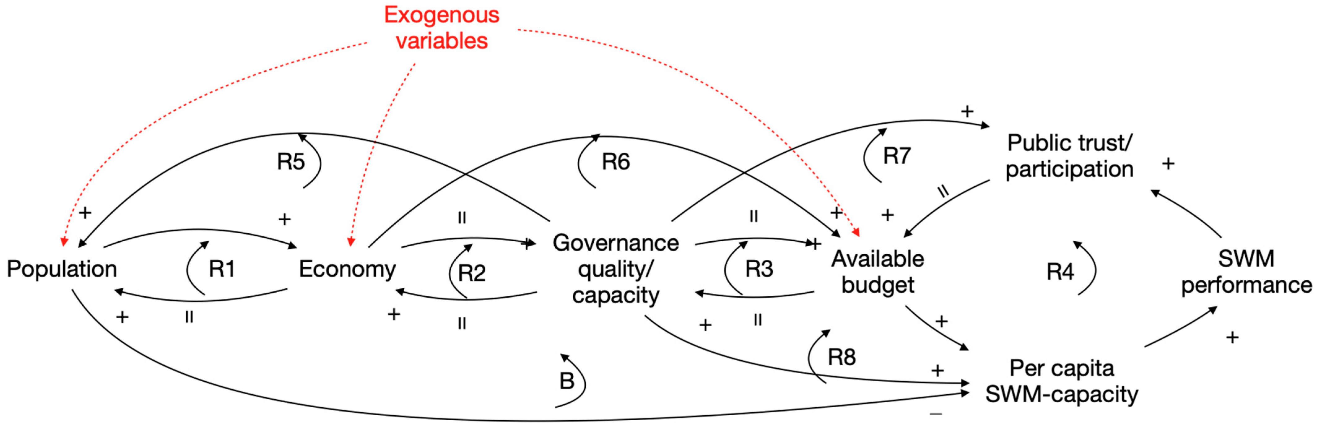
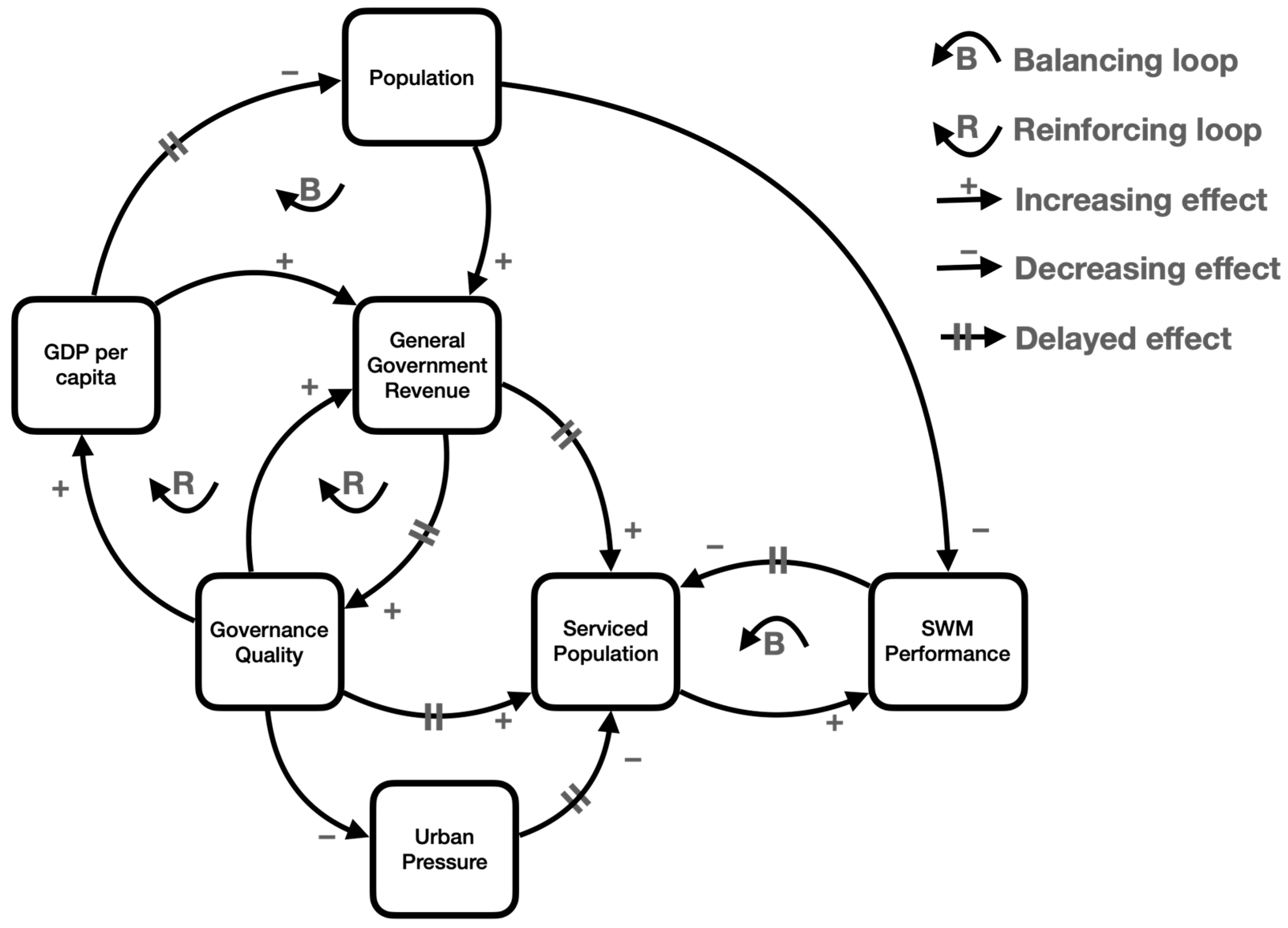
  • The target variable SWM performance (in red, SP, see Appendix B) is defined as the population being serviced (PS) divided by the total population (P). The population serviced with waste collection (PS) is positively affected by growing general government revenues (GGRs), governance quality (GQ), and public participation (PP). A negative impact may come from Urban Population Growth (UPGR) when it is beyond the level of Manageable Urban Growth (MUGR).
  • The growth of the population (P) (the variable population also covers the effects of population density as it would only need the introduction of an extra constant being a country’s surface. We chose not to do so in order to prevent the introduction of extra parameters) is influenced by GDP in such a way that a wealthier population shows declining growth rates.
  • The growth of the urban population (UP) shows the opposite behavior: a higher GDP is concentrated in the cities and attracts more citizens, leading to increased growth.
  • Governance quality (GQ) may grow as a function of increased general government revenues (GGRs) but will be limited when it nears a maximum.
  • The participation of the public (PP) is positively influenced by a higher quality of public governance (GQ).
  • The general revenues of the national government (GGRs) are ruled by the GDP of the country and by the quality of its government (GQ).
  • The GDP of the country is expressed as GDP per capita, and this variable is assumed to be influenced by the quality of government (GQ) and exogenous variables, such as the regional and international economy and international oil prices.
  • Quality of governance (GQ) is, in this model, ruled by the government’s revenues (GGRs) and political stability.
The model, constructed in this way, tries to grasp the most relevant variables and processes regarding waste collection in a country but does so at a macro level. This macro level reflects the availability of datasets that are needed to calibrate the model (see Section 2.3). It also implies that any results or conclusions from using the model cannot go deeper than this macro level. Of course, it would be interesting to be more detailed in both the model and any conclusions coming from its use. But, that can only be performed in case this detail is also reflected in the availability of detailed datasets for a country.
The system uses stock variables to describe the growth/decline in population (P), urban population (UP), public participation (PP), governance quality (GQ), and population serviced (PS). In order to keep the system simple, every stock variable is only “fueled” by one incoming flow variable, which can either be positive or negative at a certain time. Calculations for these flow variables use a general format as given below. The formula comprises basic flow rates, growth constants (describing the proportional influence of input parameters), and limiting factors (when needed).
F l o w   V a r i a b l e   x = F l o w   P a r a m e t e r b a s i c + F l o w   P a r a m e t e r c o n s t a n t V a r i a b l e   y V a r i a b l e   z L i m i t i n g   F a c t o r
All loops in the SFD include at least one delay in order to prevent simultaneous computation and use of variables. Such a delay may come from having a stock variable in the loop or from a separately imposed delay.
The SFD uses exogenous variables that impact this system from the outside in the ways described below.
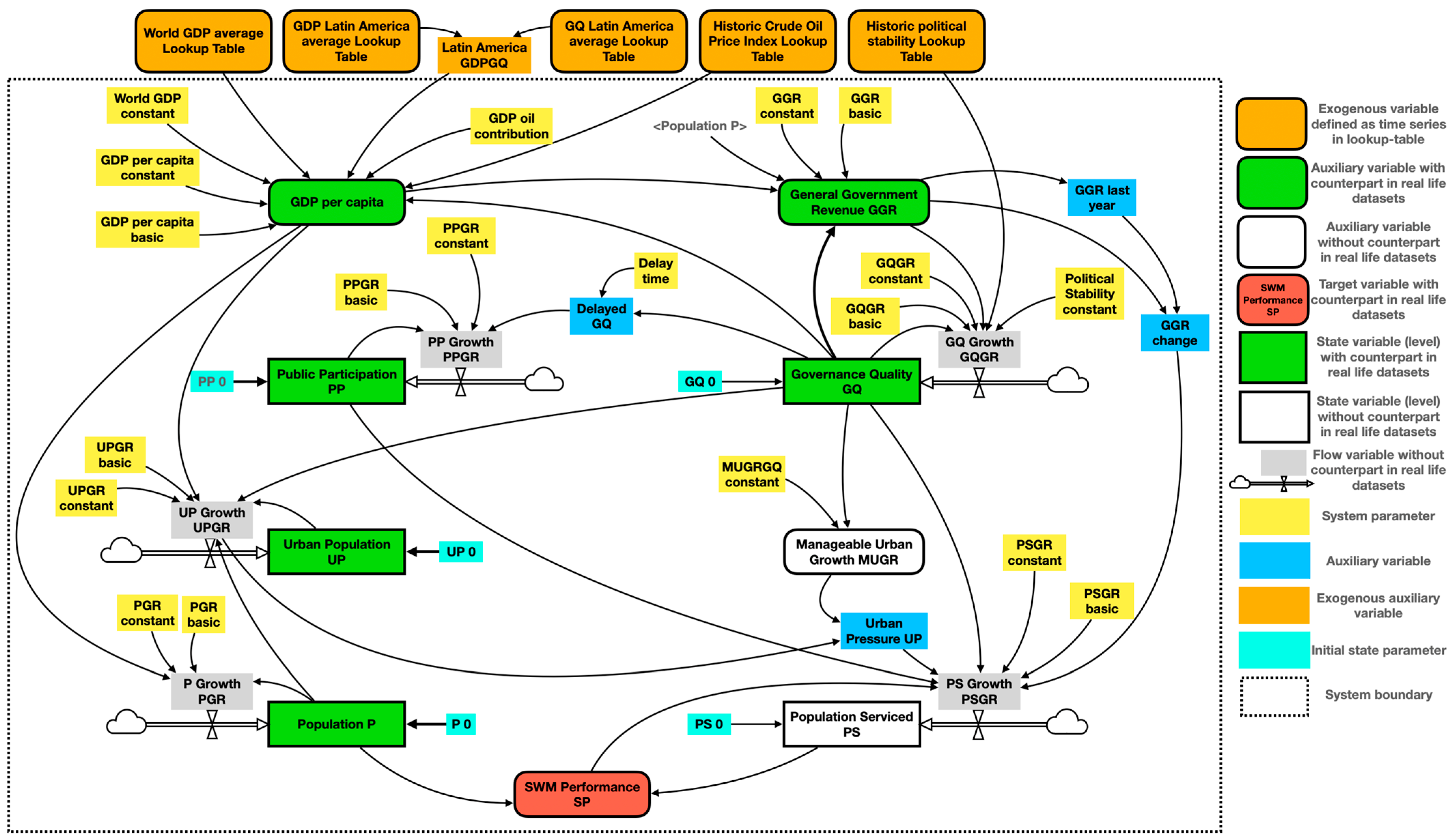
  • The influence of the world economy is introduced into the system through a lookup table. It gives the average global per capita GDP in a certain year. It serves as an input to the calculation of the country’s national GDP per capita. A parameter (world GDP constant) describes the strength of this influence on a country’s per capita GDP.
  • The model assumes that the geographic region has an impact on the economy of each country is proportional to the quality of a country’s governance. The influence of the regional economy is introduced through two lookup tables: one provides a time series for the region’s average GDP per capita and one provides a time series for the region’s average governance quality. The quotient of these lookup data (GDPGQ) is used as an input for the calculation of the country’s GDP per capita, along with a parameter (GDP per capita constant).
  • Some countries’ economies may depend very much on oil prices. For this reason, a lookup table is introduced giving the historic time series of crude oil prices for the years at hand. Also, a parameter (GDP oil contribution) rules the influence of this external variable on the GDP of each country.
  • The last exogenous variable is from inside the country. It is the political stability of a country, a variable that we considered too hard to model. For this reason, it is kept outside the system using a lookup table containing a time series for historic political stability. The time series is used as an input on governance quality. The index runs from 0 (extremely unstable) to 1 (extremely stable), and the calculation assumes that an index below 0.5 reduces the quality of governance and vice versa. A parameter (political stability constant) is used to describe the strength of this influence.

2.3. Datasets, Availability, and Selection

The primary aim of our research is to develop a diagnostic tool that can be used for developing countries around the world. Nevertheless, we anticipated and accepted that our research would be restricted to only those countries for which data would be available.
As mentioned above, the target variable SWM (solid waste management) performance is defined as the portion of the population that is serviced with regular waste collection. An internet search using the terms waste collection, data, time series, datasets, database, country, access, and statistics revealed only one source providing a time series on waste collection in developing countries, the Global Environment Statistics [46]. This database holds these series for sixty-nine countries for the years 1990–2020. The database is very incomplete and we, therefore, excluded countries with less than 4 yearly observations. The time period for calibrating the model was set to 1996–2020, as older data are generally not available. We also excluded high-income countries, small island countries, and countries with recent or ongoing conflict situations. In doing so, the list of countries is reduced to eleven. Nine of them are in Latin America (Belize, Bolivia, Brazil, Cuba, Ecuador, Panama, Paraguay, the Dominican Republic, Venezuela) and two are in Africa (Ghana and Cabo Verde). Ghana’s data appeared unreliable when comparing them to publications on actual waste collection performance and we, therefore, removed the country from our list. With only one country left in Africa, we decided to concentrate on Latin American countries only.
Time series with statistics on country-level governance quality and public participation were sought on the internet using the terms time series, datasets, database, statistics, governance, governance quality, participation, and public participation. Only the longer time series were found in the indexes of the Quality of Government Institute [47]. These time series relate to governance quality and public participation in general and not waste management specifically. Nevertheless, we decided to use both indexes as proxies in our work. As this dataset does not hold data for Brazil, Cuba, and Venezuela, we excluded these countries from our list. The focus for this study was finally set on the following six countries: Belize, Bolivia, the Dominican Republic, Ecuador, Panama, and Paraguay.
All other demographic, economic, and political data needed to feed and calibrate the model for these countries were retrieved from the World Development Indicators series of the World Bank, the IMF World Economic Outlook database, and the Global Economy website. More details on these sources are given in Appendix C.
All in all, our search for usable datasets led us to a selection of 6 six Latin American countries, for which the 7 calibration variables are available (see Table 1).

2.4. Used Software

We used Vensim Professional Version 9.3.5 ×64 (Apple Silicon, Ventana Systems Inc., Harvard, MA, USA) as the software for our modeling, simulation, calibration, and sensitivity analysis. The exact formulas used for calculating the variables in the system are given in Appendix B.

2.5. Calibration and Sensitivity Analysis

Calibrating this model means using the software described in 3.4 to find the least sum of squares for the differences between the 7 variables and their data counterparts in the time series. This is performed over the entire 25-year period by varying all of the 18 system parameters and 2 unknown initial state constants (PP 0 and PS 0; for acronyms, see Appendix B). We used the following basic settings of the software’s calibration algorithm (see also Appendix A):
  • The algorithm used a modified Powell search method to find the optimal parameter set.
  • The weighting factors for all 7 variables were kept equal. This needed a normalization step because, otherwise, a high-number variable (for example, population) would still outweigh a low-number one (for example, governance quality). Normalization was performed using the reciprocal value of the average of the variables.
  • Although data for the variables are available per year (with some hiatus), the time step in the calculations was set at 0.25 years. Further reducing this timestep did not yield significant improvements.
  • The number of new starts was set at 5000, meaning that any calibration run would include 5000 new random starting positions for the parameter sets. In doing so, each calibration run uses 5–10 million simulations for finding the weighted least sum of squares. Further increasing the number of new starts did not show any improvements.
  • All other calibration control settings were kept at the software’s defaults [48].
Additionally, a sensitivity analysis was performed for the parameter sets found in the calibration. The analysis was performed by imposing a plus and minus 10% variation on each parameter while keeping all other parameters the same. The software was then used to simulate the effect of this variation on the behavior of the target variable SWM performance (SP) during the entire 25-year period. The resulting percentual change in the target variable in the last year was used to determine whether or not a particular parameter has a strong influence on access to waste collection.

3. Results

We ran calibrations and sensitivity analyses as described in 2.5. The results comprise the following:
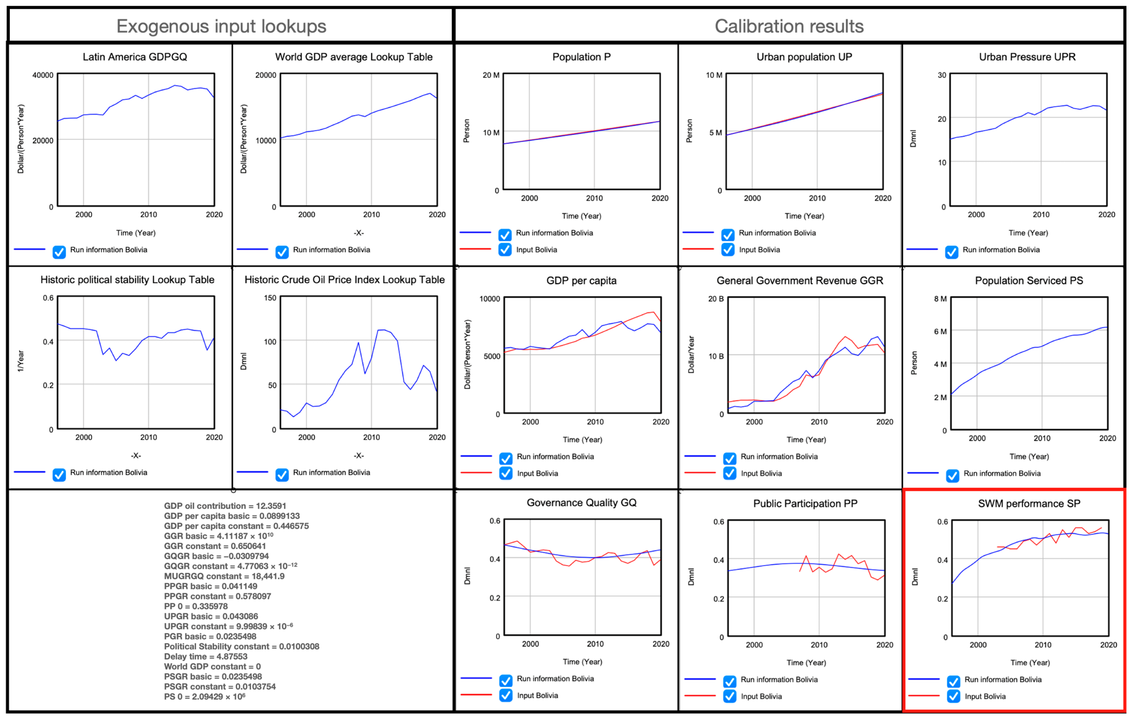
  • Calibration results for all six countries, showing the parameter values that produce the best fit to the real-life datasets;
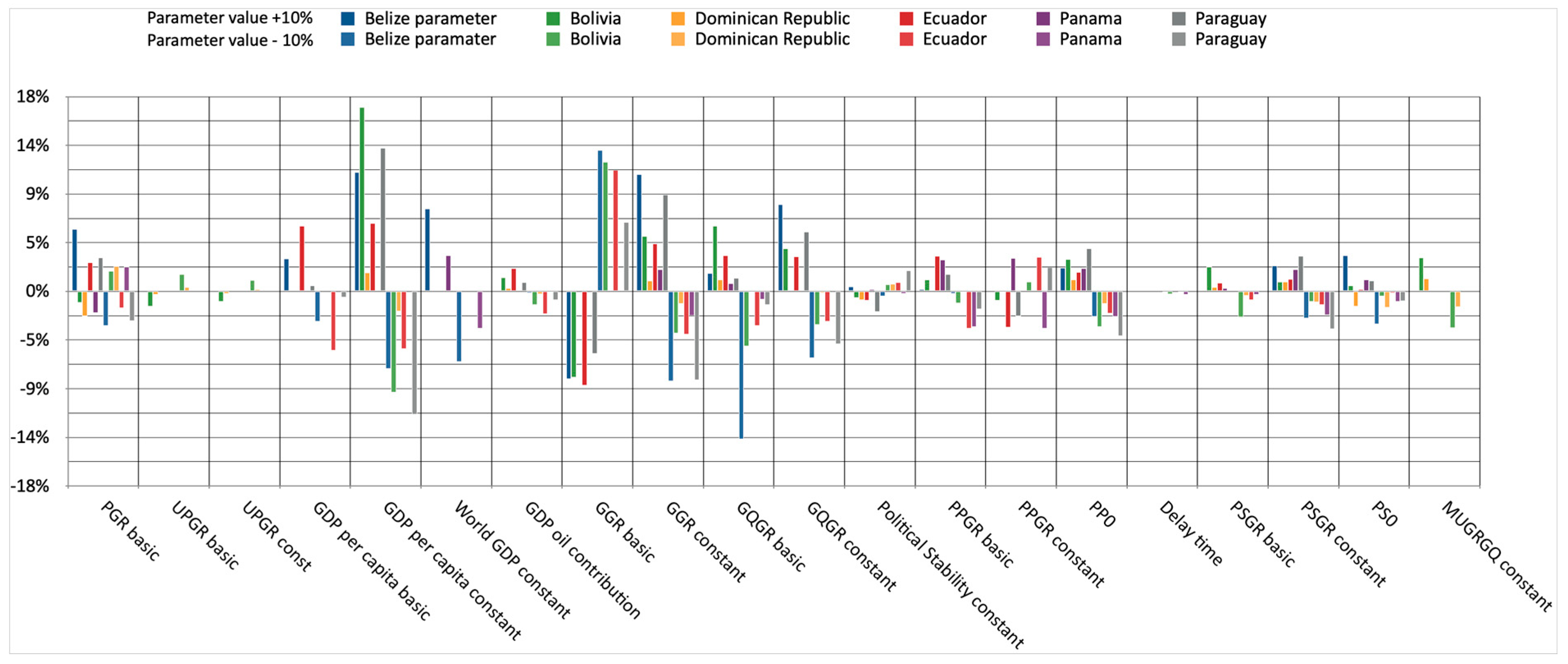
  • Sensitivity analysis for all six countries, calculating the influence of individual parameters on the target variable.
The Vensim software produces calibration results in tables and diagrams, as shown in Figure 3, for Bolivia.
Table 2 gives the results of the calibrations for all six countries. The last rows contain the graphic simulation results for the target parameter SP, the number of simulations, and the sum of weighted least squares.
The calibrations yielded good fits for all seven variables in all six countries. The question then is whether this match is based on an adequate and plausible model of the system or a coincidence? To answer this question, we compared the resulting parameters for the six countries with each other and with data from additional literature sources. A comparison between the countries needs a normalization of the parameters. The countries show large differences regarding the sizes of their populations, economies, and other dimensions. Normalization means that parameters are turned into ratios relevant to these dimensions. The normalization formulas and results are described in Appendix D. The appendix contains, in the upper part, the inputs and additional data that are used for the normalizations and background checks on the calibration results.
The sensitivity analysis yielded the results, summarized numerically in Table 3 and graphically in Figure 4. Apparently, the strongest sensitivity of the target variable is for the parameters on GDP, government revenues, and governance quality and, to a lesser extent, for those on population growth and public participation.

4. Discussion

The results will be analyzed per variable, per country, and at a consolidated level.

4.1. Per Variable

4.1.1. Population Growth and Urban Population Growth (PGR and UPGR)

The parameters used for describing the growth of the total population (PGR basic and PGR constant) produced adequate fits. In order to compare these parameters for the six countries, normalization was needed to eliminate the effect of GDP and enable combining both parameters into one growth rate. Appendix D (in the row PGR combined N) shows normalized growth rates for the six countries ranging from 1.5 to 2.5% per year. Performing the same for the growth of the urban population (UPGR combined N) leads to rates of 2 to 3.3% per year. Both these ranges are in line with the dataset. Belize shows the highest growth rates for both the total and the urban population. The lowest urbanization rate is seen in Ecuador. These results give a first indication of the effect population growth has on progress in waste collection. Belize shows zero improvement, whereas Ecuador shows the highest improvement (Table 2). This also aligns with the hypothesis from earlier studies on the relation between population growth and performance on waste collection [29,32,33].
For extra comparison, Appendix D also shows the percentages of the urban populations that lived in slums in 2018 (Appendix D, row slums 2018). One could expect that the rate of urbanization would be reflected in these percentages, and this could then be the pathway along which urbanization rates affect low access to waste collection, as postulated by [50,51,52]. For Belize, this appears not to be the case. The country has the highest rate of urbanization while showing the lowest percentage of slums. This does not mean that the model is wrong. There may be other factors that play a more dominant role in the formation of slums. But, overall, slum formation does not seem to be a decisive cause for low-performing waste collection in Belize.
The sensitivity analysis provides additional insights by showing that, indeed, population growth has an effect on the target variable SWM performance SP, but the direction of this effect can be both positive (Belize, Ecuador, Paraguay) and negative (Bolivia, the Dominican Republic, Panama). This may be due to the fact that population growth affects SWM performance SP in two different ways. There is a positive effect on the economy, leading to a higher GDP and government revenues, and another positive effect comes from higher population densities, leading to higher efficiencies in providing waste collection services. On the other hand, this is because a larger population “dilutes” the availability of budgets for SWM performance. Apparently, in Belize, Ecuador, and Paraguay, growth in budgets and efficiency of SWM services is stronger than growth in population. This dual effect was already hypothesized by [33].
The model calibrations for Bolivia show that the model’s best fit is found at very low levels of Manageable Urban Growth (Appendix D, row MUGRGQ constant N). This suggests that Bolivia is not able to absorb high influxes of new urban inhabitants and that this has an effect on the target variable. This corroborates with the data on urban slums given in Appendix D and also with research findings on the intensity of urban migration in Bolivia, which is the highest in Latin America [53]. The sensitivity analysis also suggests that the growth of the urban population only has an effect on SWM performance in countries with a limited capacity to absorb this growth, like in the case of Bolivia. This may sound trivial, but it may also support the adequacy of the model in distinguishing between countries where urbanization is or is not the root cause. The result suggests that the absorptive capacity of Bolivia’s cities is part of the bottleneck.

4.1.2. GDP per Capita

The four GDP parameters (GDP per capita basic, GDP per capita constant, GDP oil contribution, and world GDP constant; see Appendix B for acronyms) seem to be able to simulate GDP per capita. In order to make the parameters comparable and reflect their contribution to overall GDP per capita in the countries, normalizations were used as described in Appendix D. For Belize and Paraguay, the most important parameters explaining GDP growth are the ones describing the basic GDP level (Appendix D, row GDP per capita basic N) and the influence of the regional economy (Appendix D, row GDP per capita constant N). For the Dominican Republic and Bolivia, the regional economy seems to be important, but the calibration also adds some importance to the influence of oil prices (Appendix D, GDP oil contribution N). The parameters for Ecuador indicate a strong basic income level and a strong influence on the regional economy and oil prices. Overall, oil price effects are the strongest in the Dominican Republic and Ecuador. For Ecuador, this is in line with the country’s oil production (Appendix D, row oil surplus per capita). But, for the Dominican Republic, this is rather strange, as the country has to rely on imports for its oil consumption. A possible explanation may be the country’s high percentage of industry as a part of its economy [54] and the industry’s contribution to GDP having a relation with oil prices. Panama’s economy appears to be entirely tied up to the world economy (Appendix D, row world GDP constant N) and oil prices. This is in line with the country’s dependency on its canal activities and international business support, resulting in 82% of its GDP in 2017 coming from the services sector [55]. By providing good simulations and (except maybe for the Dominican Republic), apparently, for the correct reasons, this part of the model may be an important tool in predicting future developments in waste collection. Nevertheless, additional research on the adequacy of this GDP part of the model is needed to further verify these relations.
For all six countries, the sensitivity analysis shows that all GDP parameters have a strong and positive effect on target variable SWM performance. This is in line with the correlations of the World Bank on this topic [8]. The added value of the model is that it shows how this correlation translates to actual causal interactions with the other variables in the system.

4.1.3. General Government Revenue (GGR)

Here, a good fit is also achieved. On average, Belize shows a high dependency of government revenues on the country’s GDP and the quality of governance (Appendix D, row GGR combined N). The other countries show a much lower dependency. This could be a sign of a more stable revenue model for the governments in these latter countries.
When looking at GGR as a fraction of GDP (Appendix D, row GGR/GDP N), Ecuador and Belize are able to collect the most revenues and Paraguay and the Dominican Republic the least, which is in line with international studies in this field [56]. According to the sensitivity analysis, the availability of government revenues has a strong positive effect on the target variable SP. This seems to be a rather trivial outcome of the analysis. Nonetheless, there are considerable differences between the countries. For Belize, Bolivia, Ecuador, and Paraguay, this relation is very strong, whereas for the Dominican Republic and Panama, it is much weaker. Apparently, these last two countries are less able or willing to spend money on SWM services.
The literature provides little data to check the above results. The Interamerican Development Bank has released some data on spending on waste collection and treatment in Bolivia, Ecuador, and Paraguay [57,58]. For these countries, the data seem to be in line with the findings above. A recent study [59] concluded that general public spending in Latin America has increased from 19.3% to 26.3% in the period 2000–2020. When looking at the efficiency of these spendings on health, social protection, and public administration, the study concludes that low government revenues and spending do not automatically imply a low performance of these spendings. On the contrary, this last study shows that countries with the lowest spending per GDP show the highest performance of these spendings. Due to a lack of data on actual spending and efficiencies, we do not know whether this is also the case for waste services.

4.1.4. Government Quality (GQ)

The fit for governance quality is reasonably good. For Belize, Bolivia, and Panama, GQ seems to decline, which is also illustrated by the normalized results (Appendix D, row GQGR combined N). Normalizations suggest that this decline mainly comes from a basic weakness in governance quality, often in combination with political instability, as also mentioned in the literature [53]. The model suggests that in these countries, only at higher government revenues may a positive change be expected. For the Dominican Republic, Ecuador, and Paraguay, the overall situation looks more positive; however, political instability keeps playing a negative role.
The sensitivity analysis shows that GQ has an important positive effect, but there are differences between the countries. Here, the Dominican Republic and Panama show the weakest relation, meaning that improvements in governance quality do not strongly translate into better waste collection. Other factors must play a role in this inertia. To the best of our knowledge, there are no sources of other data to validate these conclusions.

4.1.5. Public Participation (PP)

The model calibration for public participation produces normalized parameters (Appendix D, PPGR basic N, PPGR constant N, and PPGR combined N; see Appendix B for acronyms), indicating a weak but still positive evolution for Belize, the Dominican Republic, and Ecuador. Bolivia and Paraguay show a negative tendency in this variable, mainly due to weak government quality. Panama shows a similar decline in public participation, but it appears to be mainly due to an intrinsically low level of public participation.
Overall, the sensitivity analysis shows that public participation has a positive but rather weak effect when compared to GDP, revenues, and governance quality. This seems to be contrary to expectations of the importance of public awareness [18]. This is most likely is due to the fact that the real-life data on waste collection used in calibration relate to the “access” and not “use” of municipal services. Or, it may turn out that the index for “Public Participation” we used in our calibrations is not a good proxy for public participation in waste collection. The literature is unclear on this. Research on the Latin American situation showed that, in general, public trust is low when compared to other global regions [60]. Nevertheless, this does not always translate into low participation; it depends on the specific type of participation. As a result, the model derived in our research may remain inconclusive regarding the importance of awareness, as long as there are no actual data on the use of municipal waste services and the actual public participation in them.

4.1.6. Population Serviced (PS)

With the exceptions of Belize and Panama, the countries show a steady increase in access to waste collection. Nevertheless, the 25-year trends in the percentage of the population being serviced seem to level off before reaching 100%. The causes for this leveling may lie in the fact that most countries have succeeded in reaching all urban citizens but face major logistical and financial problems in reaching the rural population. Another reason may be that growth in population, urban sprawl, and waste generation puts an extra burden on the organizations responsible for these services, as also reported for Latin American countries in [61].
The normalizations used for population serviced represent the annual increase in serviced inhabitants as a percentage of the total population (Appendix D, row PSGR combined N; see Appendix B for acronyms). These percentages lie between 0.6% (Belize) and 2.9% per year (Ecuador). For Bolivia, this increase seems to be somehow intrinsic; it appears to be mostly independent of government revenues. The other countries’ increases seem to be much more dependent on the additional availability of government revenues. This holds especially true for Belize and Paraguay, where growth in government revenues appears to be the only cause for growth in these services.
When dividing the annual additional budget by the number of additional serviced inhabitants (Appendix D, row GGR/PSGR N), the results implicate that in the Dominican Republic, every USD 1505 of extra government revenues leads to one extra person serviced. For Bolivia, this is USD 2844. For Belize and Panama, achieving one extra person serviced would need almost USD 10,000 of government revenues. These numbers should not be interpreted as the costs of servicing one inhabitant extra. The equation takes overall government revenues and not the revenues that are allocated for waste collection. Waste collection in Latin America costs an average of USD 10 per inhabitant [58]. Nevertheless, the results seem to suggest that waste collection has more priority in the Dominican Republic and Bolivia than in Belize and Panama, and this is in line with the progress in waste collection shown in Table 2.
For the Dominican Republic, this seems somehow contrary to the findings mentioned above under general government revenues and governance quality. Overall, the sensitivity analysis for the Dominican Republic shows a kind of “immunity” to any changes in the parameters. Apparently, there are countries, like the Dominican Republic, which can translate more budget into better waste collection but, at the same time, show an inability to further speed up this translation of “more money” into “more services”. Better quality of governance does not seem to help there.

4.2. Per Country

4.2.1. Belize

Belize shows the strongest increases in both its total and urban population. The country is able to collect substantial revenues, but this is mostly due to its population growth and is not underpinned by growth in GDP per capita. The country exhibited a steady decline in governance quality over the last 25 years, which seems to inhibit any progress in increasing the percentage of the population serviced with waste collection. Coverage has stayed at a low and steady 50% following growth in population. This seems to be corroborated by the latest available data [57] showing that, in 2021, 73% of all generated waste was being collected, assuming that urban citizens produce twice the amount of waste compared to their fellow rural citizens [8]. The country demonstrates a very low slum percentage, and this could indicate that Belize’s cities are still capable of providing sufficient formal housing to their growing urban citizens. The problem may, therefore, be that only the urban areas are included in the waste management schemes and in the statistics [17], which aligns with recent research [62]. Overlooking this situation, the conclusion could be that the quality of government is the central problem. This feeds back into the system, causing dwindling GDP per capita and a failure to set more priority on waste management, especially in rural areas. With the growth in government revenues being strongly inhibited by a lack of growth in GDP per capita and governance quality, future stagnation in waste management may be expected.
Looking at the results of the sensitivity it appears that, indeed, Belize’s waste management is primarily susceptible to increases in government revenues and governance quality. As long as governance quality is on a downward path, it will be difficult to reverse the negative development regarding SWM performance.

4.2.2. Bolivia

Bolivia shows a steady yearly increase in the percentage of serviced population, nearing 60% in 2020. Even so, a closer look reveals that the number of serviced citizens is still much lower than the number of citizens living in urban areas. This could mean that growth in waste services is mostly happening in urban areas, taking advantage of already available organizations and infrastructure and being hampered by the low absorptive capacity of the cities. Also, for Bolivia, this is in line with the findings of [57], showing that 70% of the waste is being collected. The country has the lowest per capita revenues, but its GGR/GDP fraction (Appendix D, row GGR/GDP N) is among the highest of the six countries. Although the government is apparently able to generate good revenues, governance quality and public participation are at a low and stagnant level, and this may prevent a faster increase in waste collection coverage. The work of [53] on Bolivia describes the role of social unrest on the quality of government and vice versa, as well as its negative impact on improving solid waste management in general.
This description of the situation is supported by the sensitivity analysis. There is a very strong effect of GDP on the performance of waste management services, but this variable does not provide much practical leverage for government interventions. Any effective strategy must come from improving revenues and governance related to SWM, an observation that is supported by studies in the cities of La Paz and Santa Cruz de la Sierra [31,54]. Additional research into the development of SWM revenues over the years may show whether this factor is indeed limiting progress. It may also reveal whether the absorptive capacity of Bolivia’s cities is indeed part of the bottleneck, as reported by [53].

4.2.3. Dominican Republic

The Dominican Republic is among the best-performing countries in this group. It shows some growth in the quality of government and a reasonable (but stagnant) level of public participation. The country has the lowest growth of total population but a high urbanization rate. This may have helped the country show a positive increase in the number and percentage of citizens being serviced, like in the case of Bolivia. Although government revenues are low (but firmly increasing), the country’s performance on waste collection seems to be positively influenced by a slowly increasing quality of public authorities who tend to attribute more political priority to this cause.
As mentioned above, the model for the Dominican Republic shows good performance but, at the same time, also some inertia in most of the parameters. This may indicate that the country’s progress may reside in processes not yet described in the model, such as the efficiency of municipal services or the reliance on foreign funds [54].

4.2.4. Ecuador

Ecuador’s government has been able to present stable increases in the number and percentage of people being serviced with waste collection. The total number of serviced citizens has surmounted the number of urban citizens somewhere in 2005 and seems to be leveling now at 80% of the population. The increase was possibly based on rather high and stable government revenues (partly based on oil exports) and an increase in government quality. Public participation is still at a low level but, obviously, this has not inhibited progress over the last 25 years. Nevertheless, it may now become the main inhibiting factor when aiming for 100% coverage. Indications in this direction are reported by [63]. Others found that public participation plays no role in simple basic services, such as waste collection [64]. Overall, it remains unclear whether public participation could be the limiting factor in Ecuador.
The sensitivity analysis for Ecuador shows that any progress in the field of waste management may best come from interventions that lead to improved availability of budgets. The literature reports that, indeed, Ecuador’s municipalities still have to furnish 55% of the costs of waste management from their general budgets [57,65]. More insights into the time series on the developments in financing for waste collection are needed.

4.2.5. Panama

Panama is the country with the highest GDP and government revenues. Still, government revenue as a part of GDP is rather low. The country shows weak SWM performance and only gradual increases in coverage. Only recently has the number of serviced inhabitants caught up with the number of urban citizens. This weak situation may be due to strong population growth in combination with stagnant governance quality and declining public participation. Together, these factors may also have negatively affected the political priority on spending on waste collection. This analysis is underpinned by the sensitivity analysis. It shows inertia in most of the parameters of the model.
A recent report comparing waste management in all countries of Latin America and the Caribbean [57] shows how Panama is unable to present data on its waste management performance. A total of 40% of the waste is known to be leaking into the environment, and the destination of the other 60% is unknown. It shows how the country is not in control of this part of its public services. Looking at the country’s performance on other topics, the country shows a similar low inability when it comes to closing the gaps on development issues, such as the rural/urban divide and income inequality, while better performing on education and access to tapped drinking water [66]. This could indicate that the root cause is indeed political priority.

4.2.6. Paraguay

Paraguay appears to have a low basic level of governance quality but still, the tendency is positive. The same holds for public participation. This may explain, in combination with low population growth, the country’s low but steady progress in providing citizens with access to waste collection. The low GGR/GDP fraction is apparently not limiting this progress. Nevertheless, service coverage is still among the lowest in this group. The sensitivity analysis for Paraguay reveals that interventions may best come from further improving governance quality, leading to increases in available budgets. Along with strengthened public participation, this may have a direct impact on the performance of waste collection.
Like for Panama, a recent study shows how Paraguay is unable to provide data on the coverage of its waste services. Around 60% of the waste is collected, with only 2/3 having a known destination in (uncontrolled) treatment facilities [57].
The international literature indicates that, indeed, Paraguay is doing rather well in its macroeconomic performance when compared to other countries in the region. Nevertheless, this has not translated into strong increases in income per capita and major improvements in infrastructure and education [67]. The World Bank concludes that the country has substantially lagged behind the regional averages on tax returns and other fiscal receipts and concludes that this has constrained the government’s ability to improve services and infrastructure [68]. Other sources observe that the lack of government revenues may be closely linked to the country’s weak institutions and corruption [69]. This all corroborates the conclusions from the model’s simulations.

4.3. Consolidated

The results show that the parameters of GDP, government revenues, and governance quality have the strongest influence. This behavior stems from the fact that they are part of two strong reinforcing loops, as shown schematically on the left-hand side in Figure 5. The figure also shows why the parameters on population serviced display a weaker effect; they are part of the balancing loop on the right-hand side, and this reduces their effects. Urban pressure is neither part of a reinforcing nor a balancing loop but still may have a direct effect on the target parameter.
The role of population growth is ambiguous. The need to service ever more people is a difficult task that tends to reduce the coverage percentage of waste collection. On the other side, there is a positive effect of population growth on the growth of government revenues and, in this way, it feeds into the strong reinforcing loops. Apparently, the effect of population growth on the economy and government revenues may be slower for some countries (like Bolivia and the Dominican Republic) but they are, in the end, with the help of governance quality, able to keep up with the negative effect of a growing population. As a result, the consolidated effect of a growing population may have a weak (positive or negative) effect. This is in line with an earlier statement in the Introduction of this paper where we questioned why growing economies, populations, and revenues sometimes appear to not be able to cope with growing waste volumes [28,29].
Growth of the urban population (urbanization rate) has no effect or, to put it more correctly, the model does not (need the) use of this variable and its parameters to simulate real-life data.
The parameters on government revenues and the quality of governance are important, but they have the inherent characteristic that incremental growth towards 100% collection coverage needs ever more money and government attention. This part of the system aggregates important underlying processes on the allocation of government revenues to waste management services and the efficiency of these same services for which we had no time series data. Case studies may reveal a useful time series for these aspects and may allow for an additional improvement of the model.

5. Conclusions

We were able to draw a country-level model describing how demographic, urbanization, economic, social, and governance processes affect a country’s performance on waste collection. After calibrating the parameters, the model produced acceptable fits for available datasets for all six countries and almost all variables, including the target variable.
Growth of both the urban and total population was simulated according to the real-life dataset for the six countries. Population growth shows a dual effect on the performance of waste collection: a positive effect because population growth increases economic growth and available government revenues and a negative effect because an increase in population tends to dilute the available budget per inhabitant. The combined effect appears to be positive for Belize, Ecuador, and Paraguay and negative for Bolivia, the Dominican Republic, and Panama. The speed of urbanization only seems to be a problem in Bolivia as a result of a low urban absorptive capacity.
The model seems to give a good description of growth in per capita GDP and the way it is influenced by national, regional, global, and oil-related variables. Overall, growth in GDP has a strong effect on revenues and governance quality because the variables are in an important reinforcing loop. This also seems to explain the very strong effect on the performance of waste collection. A similar effect seems to be connected to government revenues and governance quality, as these variables are in the same reinforcing loop.
Public participation is well simulated but does not seem to play an important role, which may be due to the fact that the model is simulated against data on the “access” to waste services instead of “use”. Data on the “use” of waste services are not available and may be a good subject for future research. But, it may also be the case that the variable public participation and its proxy counterpart, the data series, is too much of a catch-all index and not usable when it comes to public participation in waste collection.
The variable population serviced is well simulated but, overall, improvements in this variable don not seem to have a strong effect on the percentage of the population being serviced. This is possibly due to two effects. The first is that this variable has to “compete” with the growth of population, and the second is that incremental small growth in the number of citizens serviced comes with incremental strong growth of needed budgets. The results seem to indicate that access to the rural population may pose some kind of threshold for achieving higher percentages of access. The reasons may lie in higher costs per person and per ton of collected waste and in increased logistical challenges. Enhancing the model with these processes may lead to improvements in the model.
For Belize, the model seems to indicate that low governance quality is at the heart of the problem. Bolivia seems to reveal that the root cause may be a persistent inability to increase needed budgets and a low absorptive capacity for new urban citizens. The Dominican Republic is performing well but, overall, the country shows some inertia on all processes needed for further improvements. Panama shows an even stronger inertia and does so in a situation in which its performance is already at a strikingly low level. The results for Paraguay and Ecuador may indicate the opposite development; with low government revenues, the countries have been able to raise the quality of their governance, and this has also led to good progress in waste collection. It looks like this progress is more or less dictated by the increase in government revenues and, to a lesser extent, by public participation.
Overall, the model seems to be plausible and usable for analyzing the causes of poor SWM performance. The results may be helpful for decision makers to develop more effective (combinations of) interventions. Nevertheless, it must be stated that the model has been used for only six countries so far. And, more importantly, all six countries are located in only one global region: Latin America and the Caribbean. To test the robustness of the model, it needs to be tested in more countries and, especially, countries in other global regions.
Further research is needed to improve the model based on the following points:
  • Search for datasets for countries in other global regions and test the model against these datasets.
  • The processes describing the relation between government revenues and the actual budget for waste services.
  • The processes and variables describing the role of public participation and actual use of services.
  • The processes describing the efficiency of waste services in terms of serviced inhabitants per amount of actual budget for waste services.
  • Enhancing the model with a section on the challenges of collecting waste in rural areas.
  • A more in-depth description of the effect of urbanization and the importance of services in rural areas.
  • The availability of real-life datasets on the actual use of waste services.
  • Identifying additional variables that may enhance the model.
Such research may best be performed through case studies for individual countries or cities.

Author Contributions

The research was performed by H.B., and he also wrote the paper. H.K. and A.L. contributed by guiding the research, discussing ideas, and supervising the writing of this paper. All authors have read and agreed to the published version of the manuscript.

Funding

This research received no external funding.

Data Availability Statement

The data presented in this study are public and are available in the resources mentioned in the article (Section 2.3 and Appendix C). The data will also be made available by the authors on request.

Conflicts of Interest

The authors declare no conflicts of interest.

Appendix A. The Modeling Process

Modeling, testing, and calibrating a Stock–Flow -Diagram is mostly performed using a suitable software package. It is an iterative process, like the one given in Figure A1 for this research. Model modifications are made to remove faults by changing the structure, equations, and parameters. Testing and calibrating reveal other flaws that were not obvious before, and so the next iteration starts.
Figure A1. Iterative process for modeling, testing, and calibration used in this research. Solid arrows indicate the sequence of the process steps. Dotted arrows indicate the steps where datasets are used as input to the process.
Systems 12 00129 g0a1
Testing, calibrating, and modifying are in no way very distinct actions. In general, testing may be more about the initial stages of modeling in which the model is constructed and used as a pilot, whereas calibration is more about using the model to match real-life data. In our process, the three actions vastly overlapped. The leading principle here is that a plausible model should not only reflect a system’s real behavior but should do so for the right reasons. Therefore, a good match between model output and real-life data should not be trusted at first sight and must be tested and tried again under different premises. We refer to this iterative process as “optimization”.
In more detail, this optimization was performed in a number of ways.
  • Checking equation syntax, correct definition and the use of levels/variables/parameters, and the absence of simultaneous computation of equations. The software provides tools to perform these checks.
  • Checking units for the used levels/variables/parameters. These checks are also software enabled.
  • Using simple dummy values for the parameters and the initial state of the variables in the model. This first step is helpful to get the model running and check whether changes in parameters produce the expected behavior of variables.
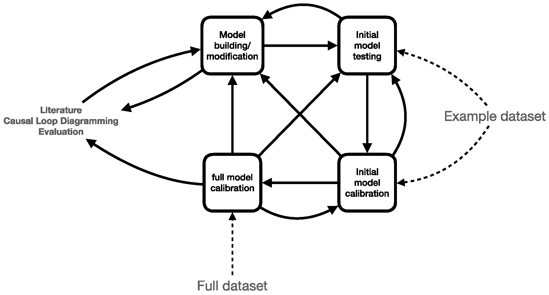
  • Using an example dataset of a single country. This enables us to check the plausibility of the model’s behavior, for example, when changing the values of the parameters (including extreme values). This can be performed by simple manual manipulation of these parameters or through running large numbers of calibration runs. Similarly, this type of testing may serve to find the minimum timestep (timestep at which further reduction does not yield changes in model behavior) that can be used for running simulations.
  • Removing redundancies. Stocks, flows, and auxiliary variables (non-essential intermediate variables that are only used to elucidate the model) are calculated through mathematical equations. In the specific case where the equation for an auxiliary variable holds parameters, there is a need for this variable to be matched with a counterpart in the dataset. If not, calibration will produce meaningless values for the parameters. In this case, these variables and their datasets may better be removed by directly connecting their inputs and outputs. This simplifies the model without affecting its performance.
  • Reality checks. If calibration of the parameter set leads to one or more absurd parameter values, it may be a good indication that there are still faults in the model structure or equations.
  • Reaching boundaries. If in calibration, a parameter value is produced equal to one of its boundary values, one should consider why this happens. It may be a miscalculated value that can be easily changed, but it may just as well be a flaw in the model.
  • Considering time delays. In case two variables are positively connected (an increase in one variable should lead to an increase in the other) but the datasets show conflicting behaviors (an increase in one variable while at the same time, the other is decreasing), the cause may be that the model does not adequately describe the delay in their cause–effect relation. This may indicate the need for introducing extra or longer delays in their connecting relations.
  • Unknown initial state of variables. In case the initial states of variables (at t = 0) are not known, these initial states can be handled as if they were parameters. In doing so, the calibration software will make the best estimate of these initial states in the same way as this calibration software is handling real parameters.
  • Critical review of available datasets. Datasets may be incomplete, unreliable, or contain outliers, leading to problems in calibration. Incompleteness can be accepted but will reduce the accuracy of calibration. Insufficient reliability, for example, based on comparison with other data or research, must, however, lead to the rejection of that set. Outliers may be considered for exclusion without rejecting the entire dataset.
  • The weighting of variables in calibration. Calibration uses the least sum of squares of the difference between calculated and real-life data for a variable. Calibration against datasets with multiple variables may need the introduction of weighting, especially when these variables have different average values. For example, the calibration against a dataset comprising the urban population and the total population of a country would emphasize the importance of the total population if no weighting were to be used. Weighting should then be performed by dividing the variables by their mean values.
  • Matching calibrated parameter values with other relevant data, insights, and benchmarks. Any resulting parameter value must be handled with skepticism, as it is only the outcome of an algorithm that handles a set of equations in order to match it with a datafile. A good match must not be trusted at first sight and must be checked as much as possible.
  • Comparing results in multiple situations. Applying the model to multiple situations (in this case, countries) can provide a good method to compare and evaluate the resulting parameter sets. Because countries differ in size, population, and so on, such a comparison needs prior normalization of the parameters.
Calibrate the calibration. Calibration of a system with n parameters is like finding a minimum in an n-dimensional space. A good match does not mean that every individual parameter is plausible, it just means that all parameters together lead to that match. This means that any calibration result must be tried by changing its starting position, extending or reducing the parameter ranges, changing the search algorithms, and reducing the time steps in order to find out if even better matches can be found. And, even then, the parameters should not be treated as valid.

Appendix B. List of Variables, Parameters, Acronyms, Units, Mathematical Equations, and Availability of Real-Life Datasets

AcronymVariable/ParameterUnitMathematical EquationAvailable Counterpart in Dataset
SPSWM Performancedmnl S P = P S / P Yes
PPopulationperson P = P   0 + 0 T P G R   d T Yes
UPUrban Populationperson U P = U P   0 + 0 T U P G R   d T Yes
PPPublic Participationdmnl P P = P P   0 + 0 T P P G R   d T Yes
GQGovernance Qualitydmnl G Q = G Q   0 + 0 T G Q G R   d T Yes
PSPopulation Servicedperson P S = P S   0 + 0 T P S G R   d T No
GDPGDP per capitadollar/(person.year) G D P = G D P   p e r   c a p i t a   b a s i c + G Q G D P G Q G D P   p e r   c a p i t a   c o n s t a n t + H i s t o r i c   C r u d e   O i l   P r i c e   I n d e x G D P   o i l   c o n t r i b u t i o n + W o r l d   G D P   c o n s t a n t W o r d l   G D P   a v e r a g e Yes
GGRGeneral Government Revenuesdollar/year G G R = G G R   c o n s t a n t G Q ( G D P P G G R   b a s i c ) Yes
MUGRManageable Urban Growthperson/year M U G R = M U G R G Q   c o n s t a n t G Q No
PGRPopulation Growthperson/year P G R = P ( P G R   b a s i c P G R   c o n s t a n t          G D P ) See P
UPGRUrban Population Growthperson/year U P G R = U P ( U P G R   b a s i c + U P G R   c o n s t a n t G D P G Q ) ( P U P ) / P See UP
UPRUrban Pressuredmnl I f   U P G R M U G R   T h e n   U P R = 1   E l s e   U P R = U P G R / M U G R No
PPGRPublic Participation Growth1/year P P G R = ( P P ( 1 P P ) ) ( P P G R   b a s i c + P P G R   c o n s t a n t D e l a y e d   G Q 0.5 ) See PP
GQGRGovernance Quality Growth1/year G Q G R = H i s t o r i c   p o l i t i c a l   s t a b i l i t y 0.5 P o l i t i c a l   S t a b i l i t y   c o n s t a n t + G Q 1 G Q ( G Q G R   b a s i c + G Q G R   c o n s t a n t G G R ) See GQ
PSGRPopulation Serviced Growthperson/year P S G R = 1 S P ( P S G R   b a s i c + P S G R   c o n s t a n t G G R   c h a n g e ) G Q P P / ( U r b a n   P r e s s u r e S P ) Yes
P 0Population InitialpersonFixed valueYes
UP 0Urban Population InitialpersonFixed valueYes
PP 0Public Participation InitialdmnlUnknown value at t=0; therefore, used as an optimization parameterNo
GQ 0Governance Quality InitialdmnlFixed valueYes
PS 0Population Serviced InitialpersonUnknown value at t = 0; therefore, used as an optimization parameterNo
GDPGQLatin American GDP/GQdollar/(year.person) G D P G Q = G D P   L a t i n   A m e r i c a   a v e r a g e G Q   L a t i n   A m e r i c a   a v e r a g e   Yes
-Delayed GQdmnl     D e l a y e d   G Q     = ( F i x e d   d e l a y   G Q ,   D e l a y   t i m e ) No
-GGR last yeardollar     G G R   l a s t   y e a r     = ( F i x e d   d e l a y   G G R ,   1   y e a r ) No
-GGR changedollar G G R   c h a n g e = G G R G G R   l a s t   y e a r No
-Urban Pressuredmnl U r b a n   P r e s s u r e = U P G R / M U G R No
-World GDP constantdmnlOptimization parameterNo
-GDP per capita constantdmnlOptimization parameterNo
-GDP per capita basicdollar/(year.person)Optimization parameterNo
-GDP oil contributiondollar/(year.person)Optimization parameterNo
-GGR constantdmnlOptimization parameterNo
-GGR basicdollar/yearOptimization parameterNo
-PPGR basic1/yearOptimization parameterNo
-PPGR constant1yearOptimization parameterNo
-Delay timeyearOptimization parameterNo
-GQGR basic1/yearOptimization parameterNo
-GQGR constant1/dollarOptimization parameterNo
-Political stability constantdmnlOptimization parameterNo
-UPGR constantperson/dollarOptimization parameterNo
-UPGR basic1/yearOptimization parameterNo
-PGR constantperson/dollarFixed at 1E−6No
-PGR basic1/yearOptimization parameterNo
-MUGRGQ constantperson/yearOptimization parameterNo
-PSGR constantperson/dollarOptimization parameterNo
-PSGR basicperson/dollarOptimization parameterNo
-World GDP averagedollar/(person.year)Lookup tableNo
-GDP Latin American averagedollar/(person.year)Lookup tableNo
-GQ Latin American averagedmnlLookup table (varies between 0 and 1)No
-Historic crude oil pricedmnlLookup table (made dmnl by dividing by USD1/barrel)No
-Historic political stability dmnlLookup table (varies between 0 and 1)No

Appendix C. Description of Variables, Ranges, and Their Sources

VariableName Used in SourceDescriptionRange/NormalizationOriginal SourceAccessed through
SWM Performance SPTotal population served by municipal waste collectionPart of population0 to 1United Nations Statistics Division[46]
Governance Quality GQGovernment effectivenessIndex−2.5 to 2.5; normalized by authors to 0 to 1Quality of Government Institute[47]
Public Participation PPCivil society participationIndex−2.5 to 2.5; normalized by authors to 0 to 1Quality of Government Institute[47]
Urban Population UPTotal urban populationNumbern.a.World Bank—World Development Indicators[70]
Population PTotal populationNumbern.a.World Bank—World Development Indicators[70]
GDP per capitaGDP per capita, purchasing power parity, 2017 international dollarsUS dollarn.a.International Monetary Fund—World Economic Outlook database[71]
General Government Revenues (GGRs)General government revenueNational currencyconverted to US dollarWorld Bank—World Development Indicators[70]
World GDP AverageGDP per capita, purchasing power parity, 2017 international dollarsUS dollarn.a.International Monetary Fund—World Economic Outlook database[71]
GDP Latin American averageGDP per capita, purchasing power parity, 2017 international dollarsUS dollarn.a.International Monetary Fund—World Economic Outlook database[71]
GQ Latin American averageGovernment effectivenessIndex−2.5 to 2.5; normalized by authors to 0 to 1Quality of Government Institute[47]
Historic Crude Oil priceBrent oil pricesUS dollar/barrelDivided by USD1World Bank[72]
Historic Political StabilityPolitical stability indexIndex−2.5 to 2.5; normalized by authors to 0 to 1World Bank[72]

Appendix D. Description of Normalizations

Normalization of calibration results for all six countries, including additional data that were used in the normalizations and the comparisons between the countries. For a description of all acronyms used, see Appendix B.
ParameterBelizeBoliviaDominican RepublicEcuadorPanamaParaguay
Normalization inputs and additional data for comparison
Oil production (1000 barrels per day) [72]2.000 × 1037.764 × 104−1.160 × 1025.484 × 1054.460 × 1024.174 × 103
Oil consumption (1000 barrels per day) [72]4.000 × 1039.000 × 1041.330 × 1052.590 × 1051.150 × 1055.100 × 104
Oil surplus per capita (1000 barrels per day)−6.513 × 10⁻³−1.272 × 10⁻³−1.410 × 10−21.985 × 10−2−3.245 × 10⁻²−7.731 × 10⁻³
Oil production per capita6.513 × 10−37.984 × 10⁻³−1.229 × 10−53.761 × 10−21.263 × 10−46.892 × 10−4
GQ average4.418 × 10−14.106 × 10−14.073 × 10−13.727 × 10−15.299 × 10−13.221 × 10⁻¹
Political stability average5.470 × 10−14.107 × 10−14.951 × 10−13.940 × 10−15.280 × 10−13.868 × 10⁻¹
Public participation average5.0834 × 10−13.5752 × 10−14.4264 × 10−12.4917 × 10−15.1379 × 10−14.5853 × 10⁻¹
GDP per capita average (USD)8.619 × 1036.611 × 1041.255 × 1041.009 × 1042.084 × 1041.011 × 104
GDPGQ average31,534
Average oil price since 1996 (USD per barrel)56
Average world GDP per capita since 1996 (USD)13,485
GGR average (USD)3.525 × 1086.481 × 1096.955 × 1092.242 × 10106.503 × 1094.032 × 109
GGR change average (USD)1.700 × 10−24.380 × 10−14.160 × 10−11.3804.570 × 10−12.750 × 10⁻¹
GGR per capita average (USD)1.148 × 1036.665 × 1027.369 × 1021.538 × 1031.842 × 1036.657 × 102
Urban population average1.397 × 1056.389 × 1066.748 × 1069.062 × 1062.285 × 1063.547 × 106
Population average3.071 × 1059.724 × 1069.439 × 1061.458 × 1073.530 × 1066.057 × 106
UPR average1.0020.3210.331.001.001.00
Slums 2018 (% of UP) [70]0.50 × 1014.850 × 1011.480 × 1012.010 × 1012.210 × 1011.710 × 101
SP average (fraction of population)4.89 × 10−14.49 × 10−17.79 × 10−17.49 × 10−16.46 × 10−13.81 × 10−1
Normalizations (N refers to normalized parameter)
GDP oil contribution N G D P   o i l   c o n t r i b u t i o n A v e r a g e   o i l   p r i c e   s i n c e   1996 / G D P   p e r   c a p i t a   a v e r a g e
5.50 × 10−31.05 × 10−11.86 × 10−11.71 × 10−11.79 × 10−26.15 × 10−2
GDP per capita basic N G D P   p e r   c a p i t a   b a s i c / G D P   p e r   c a p i t a   a v e r a g e
1.21 × 10−11.36 × 10−50.004.21 × 10−10.004.50 × 10−2
GDP per capita constant N G D P   p e r   c a p i t a   c o n s t a n t G Q   a v e r a g e G D P G Q   a v e r a g e / G D P   p e r   c a p i t a   a v e r a g e
3.92 × 10−18.75 × 10−17.79 × 10−14.04 × 10−14.35 × 10−208.65 × 10⁻¹
World GDP constant N      W o r l d   G D P   c o n s t a n t A v e r a g e   w o r l d   G D P   p e r   c a p i t a   s i n c e   1996 / G D P   p e r   c a p i t a   a v e r a g e
2.72 × 10−10.000.005.21 × 10−71.010.00
GGR basic N G G R   b a s i c G Q   a v e r a g e G G R   c o n s t a n t / G G R   a v e r a g e
1.361.698.16 × 10−21.761.088.95 × 10−1
GGR constant N G G R   c o n s t a n t G D P   a v e r a g e P o p u l a t i o n   a v e r a g e G Q   a v e r a g e / G G R   a v e r a g e
3.142.659.66 × 10−12.561.971.86
GGR combined N G G R   c o n s t a n t   N G G R   b a s i c   N
1.7819.546 × 10−18.846 × 10−18.024 × 10−18.918 × 10−19.599 × 10−1
GGR/GDP N G G R   p e r   c a p i t a   a v e r a g e / G D P   p e r   c a p i t a   a v e r a g e
1.33 × 10−11.01 × 10−15.87 × 10−21.52 × 10−18.84 × 10−26.59 × 10−2
GQGR basic N G Q G R   b a s i c G Q   a v e r a g e ( 1 G Q   a v e r a g e )
−1.93 × 10⁻²−7.50 × 10−34.48 × 10−3−4.81 × 10⁻³−1.38 × 10⁻³−8.78 × 10⁻⁴
GQGR constant N G Q G R   c o n s t a n t G Q   a v e r a g e ( 1 G Q   a v e r a g e ) G G R   a v e r a g e
9.47 × 10−37.48 × 10−35.41 × 10−48.34 × 10−28.58 × 10−54.56 × 10−3
Political stability constant N P o l i t i c a l   S t a b i l i t y   c o n s t a n t ( P o l i t i c a l   S t a b i l i t y   a v e r a g e 0.5 )
4.70 × 10⁻⁴−8.96 × 10⁻⁴−1.74 × 10⁻³−1.06 × 10−33.01 × 10−4−1.13 × 10⁻³
GQGR combined N P o l i t i c a l   S t a b i l i t y   C o n s t a n t   N + G Q G R   b a s i c   N + G Q G R   c o n s t a n t   N
−9.313 × 10⁻³−1.857 × 10⁻³−4.323 × 10−42.46 × 10−3−7.172 × 10−42.664 × 10−3
PPGR basic N P u b l i c   P a r t i c i p a t i o n   b a s i c P P   a v e r a g e ( 1 P P   a v e r a g e )
3.11 × 10−39.45 × 10−32.34 × 10−32.94 × 10−2−4.77 × 10−21.52 × 10−2
PPGR constant N P u b l i c   P a r t i c i p a t i o n   c o n s t a n t P P   a v e r a g e 1 P P   a v e r a g e ( G Q   a v e r a g e          0.5 )
−2.34 × 10⁻³−1.19 × 10⁻²−2.29 × 10⁻³−2.92 × 10−23.74 × 10−2−2.05 × 10⁻²
PPGR combined N P P G R   c o n s t a n t   N + P P G R   b a s i c   N
7.68 × 10⁻⁴−2.42 × 10−35.50 × 10−51.56 × 10⁻⁴−1.03 × 10⁻²−5.29 × 10⁻³
MUGRGQ constant N M U G R G Q   c o n s t a n t G Q   a v e r a g e / U r b a n   P o p u l a t i o n   a v e r a g e
6.92 × 10−21.19 × 10−32.47 × 10−35.14 × 10−23.22 × 10−13.23 × 10−2
PGR combined N P G R   b a s i c 1 E 6 G D P   p e r   c a p i t a   a v e r a g e
2.53 × 10−21.69 × 10−21.45 × 10−21.61 × 10−21.81 × 10−21.54 × 10−2
UPGR combined N ( U P G R   b a s i c + U P G R   c o n s t a n t G D P   p e r   c a p i t a   a v e r a g e G Q   a v e r a g e ) ( P o p u l a t i o n   a v e r a g e U r b a n   P o p u l a t i o n   a v e r a g e ) / P o p u l a t i o n   a v e r a g e
3.36 × 10−22.41 × 10−22.55 × 10−22.17 × 10−22.36 × 10−22.36 × 10−2
UPGR/PGR N U P G R   c o m b i n e d   N /   P G R   c o m b i n e d   N
1.331.421.761.341.311.53
PSGR basic N P S G R   b a s i c 1 S P   a v e r a g e G Q   a v e r a g e P P   a v e r a g e / ( P o p u l a t i o n   a v e r a g e          S P   a v e r a g e U P R   a v e r a g e )
0.001.17 × 10−28.65 × 10−37.12 × 10−31.66 × 10−30.00
PSGR constant N P S G R   c o n s t a n t G G R   c h a n g e   a v e r a g e 1 S P   a v e r a g e G Q   a v e r a g e          P P   a v e r a g e / ( P o p u l a t i o n   a v e r a g e S P   a v e r a g e U P R   a v e r a g e )
6.11 × 10−34.14 × 10−32.06 × 10−28.84 × 10−31.16 × 10−21.27 × 10−2
PSGR combined N P S G R   b a s i c   N + P S G R   c o n s t a n t   N
6.11 × 10−31.58 × 10−22.93 × 10−21.60 × 10−21.33 × 10−21.27 × 10−2
GGR/PSGR N G G R   c h a n g e   a v e r a g e / P S G R   c o m b i n e d   N P   a v e r a g e
906528441505593197323570

References

  1. Velis, C.; Mavropoulos, A. Unsound Waste Management and Public Health: The Neglected Link? Waste Manag. Res. 2016, 34, 277–279. [Google Scholar] [CrossRef] [PubMed]
  2. Sandhu, K. Historical Trajectory of Waste Management; an Analysis Using the Health Belief Model. Manag. Environ. Qual. Int. J. 2014, 25, 615–630. [Google Scholar] [CrossRef]
  3. Barles, S. History of Waste Management and the Social and Cultural Representations of Waste. In The Basic Environmental History; Springer: Florence, Italy, 2014; Volume 4, pp. 199–227. ISBN 9783319091792. [Google Scholar]
  4. Wilson, D.C.; Rodic, L.; Modak, P.; Soos, R.; Rogero, A.; Velis, C.; Lyer, M.; Simonett, O. Global Waste Management Outlook; UNEP: Nairobi, Kenya, 2015; ISBN 9789280734799. [Google Scholar]
  5. Wilson, D.C. Learning from the Past to Plan for the Future: An Historical Review of the Evolution of Waste and Resource Management 1970–2020 and Reflections on Priorities 2020–2030—The Perspective of an Involved Witness. Waste Manag. Res. 2023, 41, 1754–1813. [Google Scholar] [CrossRef] [PubMed]
  6. Maalouf, A.; Agamuthu, P. Waste Management Evolution in the Last Five Decades in Developing Countries—A Review. Waste Manag. Res. 2023, 41, 1420–1434. [Google Scholar] [CrossRef] [PubMed]
  7. Vinti, G.; Vaccari, M. Solid Waste Management in Rural Communities of Developing Countries: An Overview of Challenges and Opportunities. Clean Technol. 2022, 4, 1138–1151. [Google Scholar] [CrossRef]
  8. Kaza, S.; Yao, L.; Bhada-Tata, P.; Van Woerden, F. What a Waste 2.0, a Global Snapshot of Solid Waste Management to 2050; World Bank Group: Washington, DC, USA, 2018; ISBN 9781464813290. [Google Scholar]
  9. Niyobuhungiro, R.V.; Schenck, C.J. A Global Literature Review of the Drivers of Indiscriminate Dumping of Waste: Guiding Future Research in South Africa. Dev. South Afr. 2022, 39, 321–337. [Google Scholar] [CrossRef]
  10. Gómez-Sanabria, A.; Kiesewetter, G.; Klimont, Z.; Schoepp, W.; Haberl, H. Potential for Future Reductions of Global GHG and Air Pollutants from Circular Waste Management Systems. Nat. Commun. 2022, 13, 106. [Google Scholar] [CrossRef] [PubMed]
  11. United Nations Environment Programme. Chemicals, Wastes and Climate Change: Interlinkages and Potential for Coordinated Action; UNEP: Geneva, Switzerland, 2021. [Google Scholar]
  12. Löhr, A.; Savelli, H.; Beunen, R.; Kalz, M.; Ragas, A.; Van Belleghem, F. Solutions for Global Marine Litter Pollution. Curr. Opin. Environ. Sustain. 2017, 28, 90–99. [Google Scholar] [CrossRef]
  13. Meijer, L.J.J.; van Emmerik, T.; van der Ent, R.; Schmidt, C.; Lebreton, L. More than 1000 Rivers Account for 80% of Global Riverine Plastic Emissions into the Ocean. Sci. Adv. 2021, 7, eaaz5803. [Google Scholar] [CrossRef] [PubMed]
  14. Ferronato, N.; Torretta, V. Waste Mismanagement in Developing Countries: A Review of Global Issues. Int. J. Environ. Res. Public Health 2019, 16, 1060. [Google Scholar] [CrossRef]
  15. UN-Habitat. World Cities Report 2022. Envisaging the Future of Cities; UN Habitat: Nairobi, Kenya, 2022; ISBN 9789211333954. [Google Scholar]
  16. United Nations Department of Economical and Social Affairs—Statistics Division SDG Indicator Metadata. Available online: https://unstats.un.org/sdgs/metadata/files/Metadata-01-04-01.pdf (accessed on 10 February 2023).
  17. United Nations Statistics Division. Manual on the Basic Set of Environment Statistics of the FDES 2013 Generation and Management of Waste (Topics 3.3.1 Generation of Waste and 3.3.2 Management of Waste of the Basic Set of Environment Statistics of the FDES 2013) Elaborated by the Environment Statistics Section of the UN Statistics Division; UNSD: New York, NY, USA, 2018. [Google Scholar]
  18. Muheirwe, F.; Kombe, W.; Kihila, J.M. The Paradox of Solid Waste Management: A Regulatory Discourse from Sub-Saharan Africa. Habitat Int. 2022, 119, 102491. [Google Scholar] [CrossRef]
  19. Benito, B.; Guillamón, M.D.; Martínez-Córdoba, P.J.; Ríos, A.M. Influence of Selected Aspects of Local Governance on the Efficiency of Waste Collection and Street Cleaning Services. Waste Manag. 2021, 126, 800–809. [Google Scholar] [CrossRef] [PubMed]
  20. Salhofer, S.; Wassermann, G.; Binner, E. Strategic Environmental Assessment as an Approach to Assess Waste Management Systems. Experiences from an Austrian Case Study. Environ. Model. Softw. 2007, 22, 610–618. [Google Scholar] [CrossRef]
  21. Levis, J.W.; Barlaz, M.A.; DeCarolis, J.F.; Ranjithan, S.R. A Generalized Multistage Optimization Modeling Framework for Life Cycle Assessment-Based Integrated Solid Waste Management. Environ. Model. Softw. 2013, 50, 51–65. [Google Scholar] [CrossRef]
  22. Batista, M.; Goyannes Gusmão Caiado, R.; Gonçalves Quelhas, O.L.; Brito Alves Lima, G.; Leal Filho, W.; Rocha Yparraguirre, I.T. A Framework for Sustainable and Integrated Municipal Solid Waste Management: Barriers and Critical Factors to Developing Countries. J. Clean. Prod. 2021, 312, 127516. [Google Scholar] [CrossRef]
  23. Marshall, R.E.; Farahbakhsh, K. Systems Approaches to Integrated Solid Waste Management in Developing Countries. Waste Manag. 2013, 33, 988–1003. [Google Scholar] [CrossRef] [PubMed]
  24. Wilson, D.C.; Kanjogera, J.B.; Soós, R.; Briciu, C.; Smith, S.R.; Whiteman, A.D.; Spies, S.; Oelz, B. Operator Models for Delivering Municipal Solid Waste Management Services in Developing Countries. Part A: The Evidence Base. Waste Manag. Res. 2017, 35, 820–841. [Google Scholar] [CrossRef] [PubMed]
  25. Leal Filho, W.; Stenmarck, Å.; Kruopienė, J.; Moora, H.; Brandli, L. Benchmarking Approaches and Methods in the Field of Urban Waste Management. J. Clean. Prod. 2015, 112, 4377–4386. [Google Scholar] [CrossRef]
  26. Permana, A.S.; Towolioe, S.; Aziz, N.A.; Ho, C.S. Sustainable Solid Waste Management Practices and Perceived Cleanliness in a Low Income City. Habitat Int. 2015, 49, 197–205. [Google Scholar] [CrossRef]
  27. Guerrero, L.A.; Maas, G.; Hogland, W. Solid Waste Management Challenges for Cities in Developing Countries. Waste Manag. 2013, 33, 220–232. [Google Scholar] [CrossRef]
  28. Kalina, M. Waste Management in a More Unequal World: Centring Inequality in Our Waste and Climate Change Discourse. Local Environ. 2020, 25, 612–618. [Google Scholar] [CrossRef]
  29. Breukelman, H.; Krikke, H.; Löhr, A. Failing Services on Urban Waste Management in Developing Countries: A Review on Symptoms, Diagnoses, and Interventions. Sustainability 2019, 11, 6977. [Google Scholar] [CrossRef]
  30. World Bank. Bridging the Gap in Solid Waste Management; World Bank: Washington, DC, USA, 2021. [Google Scholar]
  31. Ferronato, N.; Gorritty Portillo, M.A.; Guisbert Lizarazu, E.G.; Torretta, V.; Bezzi, M.; Ragazzi, M. The Municipal Solid Waste Management of La Paz (Bolivia): Challenges and Opportunities for a Sustainable Development. Waste Manag. Res. 2018, 36, 288–299. [Google Scholar] [CrossRef] [PubMed]
  32. Loukil, F.; Rouached, L. Waste Collection Criticality Index in African Cities. Waste Manag. 2020, 103, 187–197. [Google Scholar] [CrossRef] [PubMed]
  33. Breukelman, H.; Krikke, H.; Löhr, A. Root Causes of Underperforming Urban Waste Services in Developing Countries: Designing a Diagnostic Tool, Based on Literature Review and Qualitative System Dynamics. Waste Manag. Res. 2022, 40, 1337–1355. [Google Scholar] [CrossRef] [PubMed]
  34. Abu-Qdais, H.A.; Shatnawi, N.; Al-Shahrabi, R. Modeling the Impact of Fees and Circular Economy Options on the Financial Sustainability of the Solid Waste Management System in Jordan. Resources 2023, 12, 32. [Google Scholar] [CrossRef]
  35. Pruyt, E. Small System Dynamics Models for Big Issues: Triple Jump towards Real-World Complexity, 1st ed.; TU Delft Library: Delft, The Netherlands, 2013; ISBN 978-94-6186-194-8. [Google Scholar]
  36. Pruyt, E. Using Small Models for Big Issues: Exploratory System Dynamics Modelling and Analysis for Insightful Crisis Management. In Proceedings of the 18th International Conference of the System, Dynamics Society, Seoul, Republic of Korea, 25–29 July 2010; pp. 1–25. [Google Scholar]
  37. Sterman, J.D. System Dynamics: Systems Thinking and Modeling for a Complex World; Working Paper Series; Massachusetts Institute of Technology: Cambridge, MA, USA, 2003. [Google Scholar]
  38. Senge, P. The Fifth Discipline. Meas. Bus. Excell. 1997, 1, 46–51. [Google Scholar] [CrossRef]
  39. Morecroft, J.D.W. Strategic Modelling and Business Dynamics; Wiley: Chichester, UK, 2015; ISBN 9781118844687. [Google Scholar]
  40. Papachristos, G. System Dynamics Modelling and Simulation for Sociotechnical Transitions Research. Environ. Innov. Soc. Transit. 2019, 31, 248–261. [Google Scholar] [CrossRef]
  41. Hürlimann, M. Dealing with Real-World Complexity: Limits, Enhancements and New Approaches for Policy Makers; Gabler Edition Wissenschaft: Wiesbaden, Germany, 2009; ISBN 9783834914934. [Google Scholar]
  42. Sterman, J.D. Business Dynamics: Systems Thinking and Modeling for a Complex World, 1st ed.; McGraw-Hill Higher Education: Boston, MA, USA, 2000; Volume 34, ISBN 0072311355. [Google Scholar]
  43. Hannan, M.A.; Hossain Lipu, M.S.; Akhtar, M.; Begum, R.A.; Al Mamun, M.A.; Hussain, A.; Mia, M.S.; Basri, H. Solid Waste Collection Optimization Objectives, Constraints, Modeling Approaches, and Their Challenges toward Achieving Sustainable Development Goals. J. Clean. Prod. 2020, 277, 123557. [Google Scholar] [CrossRef]
  44. Sterman, J.D. Sustaining Sustainability: Creating a Systems Science in a Fragmented Academy and Polarized World. In Sustainability Science: The Emerging Paradigm and the Urban Environment; Weinstein, M.P., Eugene Turner, R., Eds.; Springer Science + Business Media: New York, NY, USA, 2012; Volume 9781461431, pp. 21–58. ISBN 9781461431886. [Google Scholar]
  45. Forrester, J.W. Urban Dynamics, 1999th ed.; Pegasus Communications: Cambridge, MA, USA, 1969; ISBN 1-883823-39-0. [Google Scholar]
  46. United Nations Statistics Division Knoema.Com. Available online: https://public.knoema.com/zvpuqfe/global-environment-statistics (accessed on 28 December 2022).
  47. Quality of Government Institute Knoema.Com. Available online: https://public.knoema.com/scwzbpd/quality-of-government-institute-standard-dataset (accessed on 28 December 2022).
  48. Vensim-Systems VensimPro Manual. Available online: http://vensim.com/documentation/optimizationoptions.html (accessed on 9 May 2023).
  49. Riad Hassan, M.; Chandra Das, P.; Aminul Islam, M. Per Capita GDP and Population GROWTH NEXUS: Facts from a Cross Country Analysis. Cost Manag. 2016, 44, 39–43. [Google Scholar]
  50. Woo, B.; Jun, H.J. Globalization and Slums: How Do Economic, Political, and Social Globalization Affect Slum Prevalence? Habitat Int. 2020, 98, 102152. [Google Scholar] [CrossRef]
  51. Trindade, T.C.G.; MacLean, H.L.; Posen, I.D. Slum Infrastructure: Quantitative Measures and Scenarios for Universal Access to Basic Services in 2030. Cities 2021, 110, 103050. [Google Scholar] [CrossRef]
  52. Ooi, G.L.; Phua, K.H. Urbanization and Slum Formation. J. Urban Health 2007, 84, 27–34. [Google Scholar] [CrossRef] [PubMed]
  53. Lazo, D.P.L.; Gasparatos, A. Sustainability Transitions in the Municipal Solid Waste Management Systems of Bolivian Cities: Evidence from La Paz and Santa Cruz de La Sierra. Sustainability 2019, 11, 4582. [Google Scholar] [CrossRef]
  54. Edelman, D.J. Managing the Urban Environment of Santo Domingo, the Dominican Republic 2. The Dominican Republic 4. Poverty Alleviation Sector 6. Solid Waste Sector. Curr. Urban Stud. 2018, 7, 76–142. [Google Scholar] [CrossRef]
  55. CIA, The World Factbook – Panama. Available online: https://www.cia.gov/the-world-factbook/countries/panama/ (accessed on 15 February 2024).
  56. Gwaindepi, A. Domestic Revenue Mobilisation in Developing Countries: An Exploratory Analysis of Sub-Saharan Africa and Latin America. J. Int. Dev. 2021, 33, 396–421. [Google Scholar] [CrossRef]
  57. Alarcon Montero, P.A.; Acosta Acevedo, S.; Correal Sarmiento, M.C.; Piamonte Velez, C.; Rihm, J.A.; Breukers, L.; Duron Suarez, L.B.; Gonzalez Caballero, G.; Hernandez, C.; Sagasti Rhor, C.E.; et al. Evaluacion Regional de Flujo de Materiales; Residuos Solidos Municipales EVAL 2023; Interamerican Development Bank: Washington, DC, USA, 2023. [Google Scholar]
  58. Grau, J.; Terraza, H.; Velosa, R.; Milena, D.; Rihm, A.; Sturzenegger, G. Solid Waste Management in Latin America and the Caribbean; Inter-American Development Bank: Washington, DC, USA, 2015. [Google Scholar]
  59. Afonso, A.; Fraga, G.B. Government Spending Efficiency in Latin America. Empirica 2024, 51, 127–160. [Google Scholar] [CrossRef]
  60. Pecorari, N. Citizen Engagement and Political Trust in LAC. Master’s Thesis, Universidad de San Andres, Buenos Aires, Argentina, 2022. [Google Scholar]
  61. Margallo, M.; Ziegler-Rodriguez, K.; Vázquez-Rowe, I.; Aldaco, R.; Irabien, Á.; Kahhat, R. Enhancing Waste Management Strategies in Latin America under a Holistic Environmental Assessment Perspective: A Review for Policy Support. Sci. Total Environ. 2019, 689, 1255–1275. [Google Scholar] [CrossRef]
  62. Petterd, A.; Wander, A.; Cooney, H. Belize—Waste Data Report; CLIP, Centre for Environment Fisheries &Aquaculture Science: Lowestoft, UK, 2019. [Google Scholar]
  63. Madera Arends, R.J. Assessing the Role of Citizen Participation in Solid Waste Management (Practices) towards a Circular. Master’s Thesis, Wageningen University, Wageningen, The Netherlands, 2015. [Google Scholar]
  64. Villalba Ferreira, M.; Dijkstra, G.; Scholten, P.; Sucozhañay, D. The Effectiveness of Inter-Municipal Cooperation for Integrated Sustainable Waste Management: A Case Study in Ecuador. Waste Manag. 2022, 150, 208–217. [Google Scholar] [CrossRef]
  65. Huisman, H.; Keesman, B.; Breukers, L. Waste Management in the Latam Region; Waste Management Country Report Ecuador; Holland Circular Hotspot: Rotterdam, The Netherlands, 2021. [Google Scholar]
  66. Carlos, J.; Valdivia, R.; Gaudin, Y. Diagnostico de Las Brechas Estructurales En Panama. Una Aproximación Sistémica General; United Nations, Comisión Económica para América Latina y el Caribe: Ciudad de Mexico, Mexico, 2023. [Google Scholar]
  67. Charotti, C.J.; Valdovinos, C.F.; Soley, F.G.; Fernández, C.; Felipe, V.; Soley, G. The Case of Paraguay the Monetary and Fiscal History of Paraguay, 1960–2017; Becker Friedman Institute: Chicago, IL, USA, 2019. [Google Scholar]
  68. Canavire, G.; Corral, P.; Farfán, G.; Galeano, J.J.; Gayoso, L.; Piontkivsky, R.; Sacco, F. Modeling the Revenue and Distributional Effects of Tax Reform in Paraguay: Challenges and Lessons; Poverty & Equity Notes; World Bank Group: Washington, DC, USA, 2021. [Google Scholar]
  69. Franks, J.R.; Sab, R.; Mercer-Blackman, V.A.; Benelli, R. Paraguay, Corruption, Reform and the Financial System. Chapter 1. Has Corruption in Paraguay Contributed to Slow Economic Growth? International Monetary Fund: Washington, DC, USA, 2005; ISBN 9781589064201. [Google Scholar]
  70. World Bank, World Development Indicators. Available online: https://public.knoema.com/lftihvf/world-development-indicators-wdi (accessed on 28 December 2022).
  71. International Monetary Fund. World Economic Outlook Data. Available online: https://public.knoema.com/rwidmdc/imf-world-economic-outlook-weo-database-october-2022 (accessed on 28 December 2022).
  72. US Energy Information Agency. Theworldeconomy.Com. Available online: https://www.theglobaleconomy.com (accessed on 28 December 2022).
Figure 1. Causal Loop Diagram (CLD) describing an urban system in developing countries regarding its effects on the performance of waste collection. The arrow indicates the direction of causality, the +/− indicates the polarity of the relation, an = sign indicates delays in the relation. R refers to a reinforcing loop, which is a loop with relations that reinforce the effects. B refers to the opposite, a balancing loop.
Systems 12 00129 g001
Figure 2. The final Stock and Flow Diagram (SFD) used in this paper describing the country system with its variables, parameters, and constants, as it affects the performance of waste collection. The used colors refer to the typology of the variables and parameters given on the right-hand side. All abbreviations and relations are described in detail in Appendix B and Appendix C.
Systems 12 00129 g002
Figure 3. Example of results using Vensim, in this case for Bolivia, with the calibrated parameter set as given in Table 2. The left-hand side is the input time series used for the exogenous variables. On the right-hand side, 7 diagrams are shown for the simulated variables (blue lines) that are calibrated against real-life data (red lines), along with 2 diagrams for the auxiliary variables that are also calculated during simulations. The red-framed diagram provides the diagram for the target variable SWM performance SP. See Appendix B and Appendix C for a description of all acronyms.
Systems 12 00129 g003
Figure 4. A graphic representation of the results of the sensitivity analysis given in Table 2 for all 6 countries and all 20 parameters (PGR constant excluded). The X-axis gives the parameters, and the Y-axis gives the percentual change in the target parameter SWM performance SP when a + or −10% change is imposed on the parameters on the X-axis. For descriptions of all acronyms used, see Appendix B.
Systems 12 00129 g004
Figure 5. Schematical simplified Causal Loop Diagram of the system. Arrows indicate the direction of causality. Plus and minus indicate the polarity of the causality. An equal sign indicates delays in causality. R and B refer to reinforcing and balancing loops, respectively.
Systems 12 00129 g005
Table 1. Summary of the 6 selected countries for which datasets on the 7 calibration variables are available for the period 1996–2020.
Studied CountriesVariables Fit for Calibrating the Model
BelizeSWM Performance (SP)
BoliviaPopulation (P)
Dominican RepublicUrban Population (UP)
EcuadorGeneral Government Revenues (GGRs)
PanamaPublic Participation (PP)
ParaguayGovernance Quality (GQ)
Gross Domestic Product per capita (GDP)
Table 2. Results of parameter calibration for all six countries, including the resulting simulation of the target parameter SP, the number of performed simulations, and the resulting sum of weighted least squares.
ParameterBelizeBoliviaDominican RepublicEcuadorPanamaParaguay
PGR basic3.40 × 10−22.35 × 10−22.71× 10−22.62 × 10−23.89 × 10−22.55 × 10⁻²
PGR constant1.00 × 10−61.00 × 10−61.00 × 10−61.00 × 10−61.00 × 10−61.00 × 10⁻⁶
UPGR basic9.09 × 10−44.31 × 10−26.98 × 10−25.73 × 10−26.70 × 10−25.68 × 10⁻²
UPGR constant1.60 × 10−51.00 × 10−53.87 × 10−60.001.13 × 10−90.00
GDP per capita basic1.04 × 1038.99 × 10−20.004.24 × 1030.004.54 × 102
GDP per capita constant2.42 × 10−14.47 × 10−17.62 × 10−13.46 × 10−15.42 × 10−200.86
World GDP constant1.74 × 10−10.000.003.91 × 10−71.560.00
GDP oil contribution8.43 × 10−11.24 × 1014.15 × 1013.08 × 1016.6311.06
GGR basic1.14 × 10941.11.00 × 10101.01 × 10114.03 × 10102.95 × 1010
GGR constant9.46 × 10−16.51 × 10−11.39 × 10−11.053.29 × 10−10.38
GQGR basic−7.81 × 10⁻²−3.10 × 10−21.86 × 10−2−2.06 × 10⁻²−5.54 × 10⁻³−4.02 × 10⁻³
GQGR constant1.09 × 10−104.77 × 10−123.22 × 10−131.59 × 10−125.30 × 10−145.18 × 10⁻¹²
Political stability constant1.00 × 10−21.00 × 10−23.54 × 10−11.00 × 10−21.07 × 10−20.01
PP 04.73 × 10−13.36 × 10−14.34 × 10−12.33 × 10−14.85 × 10−10.564
PPGR basic1.25 × 10−24.11 × 10−29.50 × 10−31.57 × 10⁻¹−1.91 × 10−10.061
PPGR constant1.61 × 10−15.78 × 10−11.00 × 10−11.235.000.46
PS 01.09 × 1052.09 × 1062.73 × 1065.00 × 1061.53 × 1061.36 × 106
PSGR basic0.001.29 × 1071.65 × 1073.34 × 1063.92 × 1040.00
PSGR constant4.70 × 10−41.04 × 10−29.44 × 10−23.01 × 10−36.02 × 10−41.2 × 10⁻³
MUGRGQ constant2.19 × 1041.84 × 1044.10 × 1041.25 × 1061.39 × 1063.55 × 105
Delay time0.44.95.02.04.95.0
Resulting simulation of
SWM performance SP
Systems 12 00129 i001Systems 12 00129 i002Systems 12 00129 i003Systems 12 00129 i004Systems 12 00129 i005Systems 12 00129 i006
Number of simulations6.46 × 1064.75 × 1062.32 × 1077.40 × 1061.26 × 1071.89 × 107
Sum of weighted least squares−2.48 × 10⁻¹−1.23−1.23−1.27−1.21−1.30
Note: The model assumes that a growing GDP per capita smoothens the growth of the population [49]. The parameter PGR constant describes this relation in the way given in Appendix B. During calibrations, the optimization algorithm tended to push this parameter towards unrealistic high values. This effect could only be eradicated by setting the parameter at a fixed value. We used 1 × 10⁻⁶ person/dollar, meaning that at an average GDP per capita of a country of around USD 30,000 per person per year, population growth becomes zero. In doing so the parameter PGR constant no longer plays a role in the calibration.
Table 3. Numerical results of the sensitivity analysis for all 6 countries and all 20 parameters (PGR constant excluded). The data in the cells give the percentual change in the target parameter SWM performance SP when a + or −10% change is imposed on the parameters of column 1. A light-yellow color indicates cells with sensitivities of 5% or more. For a description of all acronyms used, see Appendix B. n.a. means “not applicable”, meaning that this parameter was calibrated at 0 during calibrations.
BelizeBoliviaDominican RepublicEcuadorPanamaParaguayBelizeBoliviaDominican RepublicEcuadorPanamaParaguay
Parameter Value +10%Parameter Value −10%
PGR basic6%−1%−2%3%−2%3%−3%2%2%−2%2%−3%
UPGR basic0%−1%−0%0%0%0%0%2%0%0%0%0%
UPGR const0%−1%−0%n.a.0%n.a.0%1%0%n.a.0%n.a.
GDP per capita basic3%0%n.a.6%n.a.1%−3%−0%n.a.−5%n.a.−1%
GDP per capita constant11%17%2%6%0%13%−7%−9%−2%−5%0%−11%
World GDP constant8%n.a.n.a.0%3%n.a.−6%n.a.n.a.0%−3%n.a.
GDP oil contribution0%1%0%2%0%1%−0%−1%−0%−2%−0%−1%
GGR basic−8%−8%−0%−9%0%−6%13%12%0%11%−0%6%
GGR constant11%5%1%4%2%9%−8%−4%−1%−4%−2%−8%
GQGR basic2%6%1%3%1%1%−14%−5%−0%−3%−1%−1%
GQGR constant8%4%0%3%0%6%−6%−3%−0%−3%−0%−5%
Political stability constant0%−1%−1%−1%0%−2%−0%1%1%1%−0%2%
PPGR basic0%1%0%3%3%2%−0%−1%−0%−3%−3%−2%
PPGR constant−0%−1%−0%−3%3%−2%0%1%0%3%−3%2%
PP02%3%1%2%2%4%−2%−3%−1%−2%−2%−4%
Delay time0%0%0%0%0%0%−0%−0%−0%−0%−0%0%
PSGR basicn.a.2%0%1%0%n.a.n.a.−2%−0%−1%−0%n.a.
PSGR constant2%1%1%1%2%3%−2%−1%−1%−1%−2%−3%
PS03%1%−1%0%1%1%−3%−0%−1%−0%−1%−1%
MUGRGQ constant0%3%1%0%0%0%0%−3%−1%0%0%0%
Disclaimer/Publisher’s Note: The statements, opinions and data contained in all publications are solely those of the individual author(s) and contributor(s) and not of MDPI and/or the editor(s). MDPI and/or the editor(s) disclaim responsibility for any injury to people or property resulting from any ideas, methods, instructions or products referred to in the content.

