Abstract
Supplier selection is a multi-attribute decision-making (MADM) problem that is affected by often-conflicting factors (e.g., price, quality, and delivery performance). If a supplier selection problem (SSP) is solved by different MADM methods, different solutions are likely to be obtained. This can be advantageous for decision makers because they have a good choice of alternative solutions. However, it brings about the need for a comparison approach for choosing the solution that best fits the decision maker’s purchasing strategy. So, decision makers may have two needs: (1) a good choice of alternative solutions and (2) a comparison approach. To help decision makers with the first need, we make two contributions to the literature on SSPs. For one, we formulate an integer nonlinear optimization model that evaluates and sorts the suppliers based on similarity to the ideal solution. For another, we make enhancements to the existing Factor Rating (FR) method. For the second need, we propose a comparison procedure to rank different solutions by measuring their relative closeness, both Rectilinear and Euclidean, to the ideal solution. The first two proposed methods along with the existing FR and TOPSIS (Technique for Order of Preference by Similarity to Ideal Solution) methods are applied to a set of test SSPs, and then, the comparison procedure is used to identify the ‘superior’ method for each test problem.
1. Introduction
Supplier selection is a MADM problem involving a number of quantitative and qualitative factors such as price, quality, and environmental impact. Dickson [1] sent a questionnaire to 273 purchasing agents and managers in the United States and Canada, and subsequently identified and ranked 23 factors for SSPs. Some factors might conflict with one another, meaning a supplier that is favorable in one factor might not be favorable in another. The relative weight or importance of these factors can differ among decision makers in the supply chain depending on their purchasing strategies [2]. The consideration of numerous factors with different weights contributes to the complexity of SSPs [3,4]. In addition, the cost of component parts and raw materials in manufacturing can be up to 70% of product cost [5]. In such circumstances, supplier selection is a strategic decision and one of the most important functions of purchasing management [6].
There exist two scenarios in SSPs: single sourcing and multiple sourcing. In the first scenario, all candidate suppliers are individually capable of meeting a buyer’s needs, and therefore, it would suffice for the buyer to select a single supplier. In the second scenario, supplier constraints (e.g., production capacity) force a buyer to purchase the same item from more than one supplier. Also, multiple sourcing is a practical way of ensuring the reliability of a buyer’s supply stream [7]. For example, Toyota, Honda, and Nissan were affected by the devastating Japan earthquake and tsunami in March 2011, partly due to the disruptions faced by their Japanese parts suppliers. In this case, a buyer might prefer to split its orders among multiple suppliers who are, for example, geographically scattered even though single sourcing is possible. Typically, in multiple sourcing, the buyer can first rank the suppliers by an MADM method and then split the order among the ranked suppliers, with greater quantities ordered from the higher-ranked suppliers as capacities permit.
2. Literature Review
The various solution methods that have been applied to SSPs include the analytic hierarchy process or AHP [8,9], analytic network process or ANP [10], linear weighting methods [11,12], total cost approach [13], TOPSIS [14,15], machine learning algorithms [16], and mathematical programming techniques [4,17].
Among these methods, TOPSIS is one of the widely used techniques that evaluates and ranks suppliers based on the concept that the chosen alternative should have the shortest distance from the positive ideal solution (PIS) and the longest distance from the negative ideal solution (NIS). It is worth noting that TOPSIS is a variation of the classical Hellwig’s method [18] that dates back to 1968. TOPSIS considers distances to the ideal and anti-ideal, while Hellwig’s method considers only distances to the ideal.
Modibbo et al. [19] performed a multi-criteria decision analysis for pharmaceutical supplier selection using Fuzzy TOPSIS. Memari et al. [20] used Fuzzy TOPSIS for sustainable supplier selection. Junior et al. [21] developed a comparative analysis of Fuzzy TOPSIS and Fuzzy AHP methods in the context of supplier selection decision-making. Singh et al. [22] proposed a hybrid model of Fuzzy AHP and Fuzzy TOPSIS to evaluate and select an appropriate third-party logistics (3PL). Yu et al. [23] developed a novel integrated supplier selection approach incorporating a buyer’s risk attitude using the artificial neural network, AHP, and TOPSIS methods. Venkatesh et al. [24] applied integrated fuzzy AHP and TOPSIS methods to evaluate and rank supply partner alternatives. Leong et al. [25] integrate GRA (Grey Relational Analysis), BWM (Best Worst Model), and TOPSIS for resilient supplier selection.
Luan et al. [26] combined a genetic algorithm and ant colony optimization to solve a supplier selection problem. Zakeri et al. [27] proposed a method of evaluating suppliers based on optimal points and win–loss–draw decision-making. Stević et al. [28] present a method for sustainable supplier selection in healthcare industries they call MARCOS, for measurement of alternatives and ranking according to compromise solution. FR, also known as the simple additive weighting method, is another MADM method that has been used for facility location, scholarship applicant, and IT-project selection problems by researchers such as Sharma et al. [29] and Rizana and Soesanto [30].
Awasthi et al. [31] studied a multi-tier, global supplier selection problem using a fuzzy AHP-VIKOR-based approach. VIKOR is a Serbian acronym that translates to multi-criteria optimization and compromise solution. VIKOR uses vector normalization of criterion units, whereas TOPSIS uses linear normalization. Rajesh and Ravi [32], as well as Golmohammadi and Mellat-Parast [33], developed Grey relational analysis-based models for supplier selection. Hashemi et al. [34] combined the analytic network process and Grey relational analysis for supplier selection. Tsai et al. [35] developed a fuzzy data envelopment analysis model, while Wang et al. [36] combined DEA and Grey’s, for supplier selection and plant site selection, respectively.
We summarize the literature review in Table 1 where LWM is linear weighting methods; TCA is total cost approach; MLA is machine learning algorithms; MP is mathematical programming; and OM is other methods.

Table 1.
The literature review.
3. Research Focus
SSPs are akin to, say, forecasting problems in the sense that different methods can be used to generate solutions. As these methods produce different forecasts, alternate measures (e.g., mean absolute deviation and mean squared error) can be used to evaluate the forecast methods and select the one that best meets the forecaster’s overall strategy. The same can be said for MADM problems like SSPs: they can be solved by different MADM methods, resulting in different alternative solutions. Having a good choice of alternative solutions may be advantageous for the decision maker but a comparison approach is needed for picking the solution that best fits the desired purchasing strategy. So, decision makers may have two needs: (1) a good selection of alternative solutions and (2) a comparison approach for identifying the ‘best’ solution.
To help decision makers with the first need, we propose two new methods to evaluate and rank suppliers. The first new method involves the formulation of an integer nonlinear optimization model that evaluates and sorts the suppliers based on similarity to the ideal solution. We call the model INOSIS (Integer Nonlinear Optimization by Similarity to the Ideal Solution). The INOSIS method is based on the TOPSIS concept. For the second new method, we make enhancements to the existing Factor Rating (FR) method and call it the Modified Factor Rating (MFR) method. Our main objective of proposing the INOSIS and MFR methods is to complement the methods mentioned in the literature review and to provide more alternative solutions for decision makers. In this study, we show that no method consistently provides the most preferred/desirable solution.
For the second need, we propose a procedure referred to as ROS, for Ranking-of-Solutions, to rank different solutions by measuring their relative closeness, both rectilinear and Euclidean, to the ideal solution. The ROS procedure assumes that the decision maker would prefer a supplier that is closer to (or more resembles) the best-possible supplier compared to the other suppliers. It is believed to be the first of its kind that helps the decision maker identify which solution is most preferred.
In Section 4 of this paper, the single-source problem under study is defined, the proposed MFR and INOSIS solution methods and proposed ROS selection procedure are described. In Section 5, the FR, MFR, INOSIS, and TOPSIS methods are applied to a set of test SSPs, and the ROS procedure is used to rank their solutions. In Section 6, conclusions are drawn and suggested future research is discussed.
4. Methods
The two proposed SSP solution procedures, MFR and INOSIS, as well as the proposed ROS procedure are described in detail next. The following notations are used in the proposed methods:
| S = {, …, , … } | discrete set of m possible suppliers |
| Q = {, …, , … } | discrete set of n factors |
| W = {, …, , … } | vector of n factor weights |
| weight assigned to factor | |
| NWi | normalized weight calculated for factor |
| rating of supplier j for factor i | |
| D | decision matrix containing |
| NRij | normalized rating of supplier j for factor i |
| ND | normalized decision matrix containing NRij |
| converted normalized rating of supplier j for factor i | |
| CND | converted normalized decision matrix containing |
| Oj | overall score of supplier j |
| positive ideal solution | |
| Ej | weighted distance of supplier j from |
| best-possible rating | |
| worst-possible rating | |
| αij | rating’s relative closeness to the best-possible rating |
| SCSj | weighted relative closeness score of supplier j |
| OCS | overall closeness score |
4.1. Preliminary Steps
The four SSP solution methods (FR, MFR, TOPSIS, and INOSIS) employed in this paper all start with the seven steps described below.
Step i. Decide on the set of candidate suppliers, where S = {, …, , … } is a discrete set of m possible supplier alternatives.
Step ii. Decide the supplier factors (e.g., price, quality, and location) to be considered, where Q = {, …, , … } is a discrete set of n factors. It is assumed there are i = 1 to positive (or benefit) factors like reputation and i = 1 to negative factors like wholesale price.
Step iii. Decide the factor weights to be used, where W = {, …, , … } is a vector of n factor weights and is the weight assigned to factor . Decision makers usually use linguistic variables to express the factor weights. For example, the environmental impact of a supplier can be very low, low, moderate, high, or very high. In such a case, the factor weights can be expressed by the 5-level scale shown in Table 2.
Table 2.
Scale of factor weights.
Step iv. Normalize the factor weights. The sum of the weights should equal one, and thus they are normalized by Equation (1), getting :
Example: Assume that a buyer is evaluating three suppliers against two factors: is service level that is a positive, qualitative factor; is wholesale price that is a negative, quantitative factor. Based on the buyer’s strategy, the importance of is “Very High” meaning . Or the importance of is slightly lower than “Moderate” which means somewhere between “Moderate” and “Poor” but closer to “Moderate”. So, from Table 2, the weight can be a number between 0.25 and 0.50 but close to 0.50. How much closer this is to or far from “Moderate” (or 0.50) depends on the decision makers’ discretion. So, the decision makers may set to . Table 2 is intended to show five discrete reference points on a continuous zero-to-one scale. By applying Equation (1), the resulting normalized weights, NW1 and NW2, are 1.00/1.43 = 0.7 and 0.43/1.43 = 0.3, respectively.
Step v. Decide on the quantitative scale to be used for the rating values of the m suppliers on the n factors. Decision makers often start with linguistic variables to express the scale for supplier factor ratings. The linguistic variables are then converted to quantitative values. Table 3a,b are two examples of how conversion can be accomplished, the former for monotonic variables and the latter for non-monotonic variables.
Table 3.
(a) Scale of supplier factor ratings for a factor with monotonic levels. (b) Scale of supplier factor ratings for a factor with non-monotonic levels.
A monotonic factor, such as product quality, has strictly increasing or strictly decreasing levels. The optimal level is the minimum or maximum level. In contrast, a non-monotonic factor, such as supplier capacity utilization, has both increasing and decreasing levels. A non-monotonic supplier variable is analogous to a concave or convex utility function. The optimal level is not necessarily the maximum or minimum level. The classic Economies/Diseconomies of Scale concept that arises in operations management is an example of a non-monotonic scale.
Keep in mind, both Table 3 (a,b) happen to show just five discrete reference points on a continuous 0 to 100 scale.
Step vi. Decide rating values Rij, where is the rating of Supplier j for factor i. For qualitative factors, use Table 3 to identify the factor rating values for each supplier. Quantitative factors are scaled using their own real numbers.
Step vii. Construct decision matrix D as shown in Equation (2).
4.2. Modified Factor Rating (MFR) Method
The MFR method is like the Factor Rating (FR) method in that it is used for evaluating and ranking alternatives against multiple factors. As the factors may have different scales or units, they need to be normalized. Furthermore, all the factors need to be converted to the same classification of either positive or negative. In the FR method used by Rizana and Soesanto [30], normalization and conversion are performed in one step (which is presented in Appendix A). However, in the MFR method, normalization and conversion are performed differently and separately. The difference between FR and MFR has a considerable impact on the solution and is discussed in the numerical analysis section. We explain the MFR method in this subsection, while the FR method is covered in Appendix A.
MFR Procedure
We continue with the example problem introduced in Section 4.1 involving three candidate suppliers and two factors, service level (a positive factor) and wholesale price (a negative factor). The execution of Steps i through vii, described above, resulted in the following decision matrix D:
Here, one can see that Supplier 2 is offering the highest service level, 0.75, and Supplier 3 is offering the lowest wholesale price, $95.
Step 1. Normalize the ratings to get NRij using Equation (3) and construct the normalized decision matrix in Equation (4):
Note: The factor ratings are normalized to transform the different factor scales into a common measurable scale to allow comparisons across the factors.
Applying Equation (3) to the service factor Q1 ratings: NR11 = 0.25/1.25, NR12 = 0.75/1.25, and NR13 = 0.25/1.25. Applying it to the price factor Q2 ratings: NR21 = 100/305, NR22 = 110/305, and NR23 = 95/305. The resulting normalized decision matrix ND is:
Step 2. If any factor is negative, as is the case with wholesale price factor Q2, the factor’s ratings must be converted to positive by means of Equation (5). The resulting converted normalized decision matrix CND is denoted by Equation (6).
Q2 is a negative factor, so the complements of the three suppliers’ normalized ratings are found to be 0.672, 0.639, and 0.689. In this instance, the complementary ratings sum to 2 (i.e., ), so if each complementary rating is divided by 2, we have . Q2’s normalized ratings are CNR21 = 0.3360, CNR22 = 0.3195, and CNR23 = 0.3445. The resulting converted normalized decision matrix, CND, is:
If a fourth supplier were added, the sum of the complementary ratings for the four suppliers would be To generalize, we always have . Therefore, we can normalize the complementary ratings by dividing them by , i.e., .
Step 3. Calculate each supplier’s overall score Oj by Equation (7):
Continuing with the example and using Equation (7), the resulting overall scores of the three suppliers are:
Step 4. Rank the suppliers in decreasing order of their overall scores. The supplier with the highest overall score is the best-choice supplier. In this example, Supplier 2 is the best choice, Supplier 3 is the second best, and Supplier 1 is the third best.
4.3. Integer Nonlinear Optimization (INOSIS) Model
For the INOSIS model, we formulate an integer nonlinear optimization model to evaluate and sort the suppliers. The model does so based on the TOPSIS concept that the chosen alternative should have the shortest Euclidean distance from the positive ideal solution, PIS. The INOSIS model maximizes the sum of the products of the suppliers’ ranking and the suppliers’ distance from the PIS. A larger rank is assigned to a longer distance, and conversely, because it is a maximization model. So, the suppliers are sorted in the increasing order of the rankings obtained by the INOSIS method.
The INOSIS model requires execution of Steps 1 and 2 described in Section 4.2 for the MFR method. Thus, our discussion of the INOSIS model assumes the ratings have been normalized and negative-factor ratings have been converted to positive ratings (i.e., the CND matrix is completed).
Step 3. Determine the PIS, denoted , from the converted normalized decision matrix , where .
Step 4. Compute the weighted distance of Supplier j from , denoted Ej, using Equation (8).
where k = 1 and 2 are used for rectilinear and Euclidean distances, respectively.
Step 5. Formulate and solve the following integer nonlinear optimization model represented by Equation (9) through (12).
subject to
Equation (9) makes sure that is assigned to the smallest , to the second smallest , … and to the largest . Let us assume there are two suppliers (j = 1, 2), where is an integer decision variable and represents supplier j’s ranking. indicates that Supplier 2 is superior to Supplier 1, and thus, and . Since and , we have . So, the largest possible value for results when we assign the largest (i.e., ) to the largest (i.e., ) and the second largest (i.e., ) to the second largest (i.e., ). Therefore, the ranking of the suppliers, , can be obtained by maximizing Equation (9), subject to the constraints represented by Equations (10)–(12).
Equation (10) indicates that are strictly positive integer values. Equation (11) ensures that no two suppliers have the same ranking.
Equation (12) prevents from becoming infinite as Equation (9) is maximized. To see how Equation (12) works, assume that there are four suppliers (i.e., m = 4), where . For m = 4, we have for Equation (12). Here, one can see that, since each supplier’s ranking must be unique and strictly positive integer, the only possible values for to make are 1, 2, 3, and 4.
Step 6. Rank the suppliers in the increasing order of the (since the smallest is assigned to the smallest , the second smallest to the second smallest , etc.).
4.4. Ranking of Solutions (ROS) Procedure
Here, it is assumed a buyer prefers a supplier that is closest to (or most resembles) the theoretical best supplier and supplier rankings are based on this preference. (In the example introduced in Section 4.1, the ratings of the theoretical best supplier for and are 0.75 and $95, respectively.) To be general as well as consistent with the TOPSIS and INOSIS methods, the proposed ROS procedure measures the weighted relative closeness (in both rectilinear and Euclidean distance) of a solution to the ideal solution.
Step 1. We express the suppliers’ ratings, , in the decision matrix D, by fuzzy sets whose membership function increases linearly from 0 to 1 as shown in Equation (13) and Figure 1. The membership function is 1 for the best-possible rating, , and 0 for the worst-possible one, . For positive factors, and , and for negative factors, and .
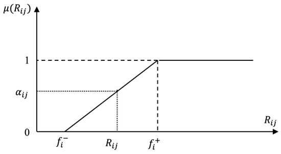
Figure 1.
Membership function for supplier rating, .
Step 2. Compute each rating’s relative closeness, αij, to the best-possible rating, using Equation (14):
Step 3. Compute each supplier’s weighted relative closeness score, SCSj, by Equation (15):
where k = 1 for rectilinear and k = 2 for Euclidean, relative closeness.
The supplier’s ranking, obtained by the evaluation method in question, must be included in this calculation by means of a Gj score. Score is assigned to Supplier j, , so that an inferior supplier cannot be scored greater than its superior. For example, if Supplier j is the best supplier, if Supplier l is the second-best supplier, and so on.
Step 4. Compute the overall closeness score, OCS, by Equation (16):
In Equation (16), one can see that smaller values of OCS are desirable because when gets closer to , OCS gets smaller.
Step 5. Rank the supplier selection methods in increasing order of their overall closeness scores. The method with the smallest OCS is the one preferred by the buyer.
5. Numerical Analysis
The FR, MFR, INOSIS, and TOPSIS methods, as well as the ROS procedure, were applied to a supplier selection problem involving 7 suppliers and 12 factors. The steps of the MFR method are presented, but only the results of the FR, INOSIS, and TOPSIS methods are shown to keep this paper concise. Then, we present a summary of the results of applying the four solution methods and ranking-of-solutions procedure to 100 test problems whose parameters were generated randomly in MS Excel.
5.1. Single Test Problem
5.1.1. Preliminary Steps
Step i. It is assumed there are seven suppliers (m = 7).
Step ii. It is assumed there are twelve factors (n = 12). The first six factors are assumed to be positive ( = 6) and the other six (n − = 6) are negative. The positive factors might include supplier production capacity and product-option variety because higher values for these factors would likely be more appealing to buyers. The negative factors might include supplier wholesale price and product defective rate, for which buyers would likely prefer lower values.
Step iii. In practice, the weight of each of the twelve factors is decided by the buyer. For this demonstration, the weights were randomly generated in MS Excel using “RANDBETWEEN(0, 100)/100”.
Step iv. The weights are normalized by Equation (1) and appear in Table 4.
Table 4.
Normalized factor weights.
Steps v and vi. In practice, the supplier ratings for each factor are decided by the buyer. For this demonstration, the suppliers’ ratings for the twelve factors were randomly generated by the “RANDBETWEEN” function in MS Excel. For example, the suppliers’ ratings for the first factor was generated by “=RANDBETWEEN(8, 10)”. For the remaining eleven factors, the values “(0, 100)”, “(0, 1)”, “(0, 1)”, “(8, 10)”, “(5, 12)”, “(5, 20)”, “(0, 1)”, “(0, 1)”, “(0, 1)”, “(0, 1)”, and “(20, 50)” were used as the lower and upper bounds, respectively, in the “RANDBETWEEN” function.
Step vii. The resulting decision matrix D containing the supplier ratings for the 12 factors appears in Table 5.
Table 5.
Decision matrix D containing Rij values and each factor i’s .
5.1.2. MFR Procedure
Steps 1 and 2. Using Equations (3) and (5), the converted normalized decision matrix CND in Table 6 is computed.
Table 6.
Converted normalized decision matrix, CND.
Step 3. The suppliers’ overall scores for the MFR method are computed by Equation (7) and shown, along with their subsequent rankings, in Table 7. Table 7 also shows the results of the other three methods.
Table 7.
Overall score and ranking of each supplier for the four methods.
The INOSIS model was formulated in MS Excel and solved by Solver and finds only the supplier rankings, not the scores. For the FR, MFR, and TOPSIS methods, the supplier with the highest overall score is the best supplier. For example, for the MFR method Supplier 3’s overall score is the highest (i.e., , and thus it has a ranking of “1”.
5.1.3. ROS Procedure
For this particular problem, all four solution methods ranked Supplier 3 as “1”, but the methods differed in their other supplier rankings, which would be meaningful if this was a multiple-source SSP and prompts the application of the proposed ROS procedure.
Steps 1. From Table 5, we obtain the best-possible rating, , and the worst-possible one, , shown in Table 8. For positive factors, and , and for negative factors, and .
Table 8.
The best- and the worst-possible ratings.
Step 2. Using Equation (14), the ratings’ relative closeness, , to the best-possible ratings are calculated and shown in Table 9.
Table 9.
The relative closeness, , to the best-possible ratings.
Step 3. Using Equation (15) and k = 1, each supplier’s weighted relative closeness score, SCSj, is computed and shown in Table 10.
Table 10.
The suppliers’ weighted relative closeness scores.
Step 4. Using Equation (16), the overall closeness score, OCS, is computed to be 11.35.
The overall closeness score, OCS, for the other three methods was found to be (in ascending order) 11.44 for FR, 11.51 for TOPSIS, and 11.56 for INOSIS. In this instance, the MFR method is superior because its overall closeness score is the lowest. When k = 2, the OCS scores were 0.94 for MFR, 0.96 for FR, 0.95 for TOPSIS, and 0.99 for INOSIS, again resulting in the MFR method being superior.
5.2. Set of 100 Test Problems
To have a robust analysis, random numbers were generated in MS Excel to produce the supplier factor ratings and factor weights for 100 cases involving 7 suppliers and 12 factors. For each case, the four methods were used to score and rank the suppliers. Then, the ROS procedure was employed to measure their effectiveness and determine the superior method. Table 11 shows the number of times each of the four methods was, or tied for, the superior method.
Table 11.
Number of times each of the four methods is superior.
The results show that the FR method provided superior (most preferred) solutions far more frequently than the other three methods when k = 1. However, when k = 2, TOPSIS provided superior solutions nearly as frequently (40 times) as did the top-performing FR method (42 times). No method tested was consistently superior, which is why the decision maker can benefit from using a number of methodologies and picking the solution that best fits their purchasing strategy.
6. Conclusions and Suggestions for Future Research
A host of different methods for evaluating and ranking suppliers has appeared in the literature. When a SSP is solved by those methods, different solutions are likely to be obtained. This can be advantageous for decision makers because they have a good choice of alternative solutions. However, this may bring a question that what solution can be the superior/most-preferred one. In other words, decision makers need a comparison approach for choosing the solution that best fits their purchasing strategy or that is the superior/most-preferred solution. To help the decision makers with this need, a ROS procedure was proposed here.
In this study, we applied four SSP solution methods, two proposed (MFR and INOSIS) and two established (FR and TOPSIS) ones, to 100 test problems whose parameters were generated randomly in MS Excel. As expected, the solutions (i.e., supplier rankings) determined by the four solution methods often varied in the case of each test problem. Then, we used the proposed ROS method to determine the superior/most-preferred solutions. The analysis on the 100 test problems showed no method was consistently superior or provided the superior/most-preferred solution. Therefore, our main objective of proposing the INOSIS and MFR methods is to provide a good choice of alternative solutions for the decision makers. And the reason for proposing the ROS method is to determine the superior/most-preferred solutions.
Based on the analysis, it is suggested that different methods be used to solve a problem and that the ROS procedure be used to realize which solution is preferred. More robust testing of solution methods and the proposed ROS procedure would be worthwhile.
There might still be methods, new or modified, that can be developed for the multi-attribute supplier selection problem defined in this study. In addition, the proposed ROS procedure is but one way to evaluate the solutions of the different MADM methods; the development of other approaches could be beneficial.
For future research, it might be worthwhile to investigate how the uncertainty of, or changes in, suppliers’ performance on the various evaluation criteria can be considered in the supplier ranking process. For example, the quality of a raw material purchased from Supplier 1 is currently better than Supplier 2. However, the quality of Supplier 1 is getting worse over time while that of Supplier 2 is getting better. A stochastic approach to scoring supplier performance might be a realistic consideration. Going further, sensitivity (i.e., what-if) analysis could be conducted to determine the change in supplier rankings that results from changes in performance criteria weights or scores.
Author Contributions
All authors contributed to the paper’s conceptualization, new methodology development, formal analysis, validation of results, original draft writing, and paper refinement/editing. All authors have read and agreed to the published version of the manuscript.
Funding
This research received no external funding.
Data Availability Statement
The original contributions presented in the study are included in the article; further inquiries can be directed to the corresponding author.
Conflicts of Interest
The authors confirm that there are no relevant financial or non-financial competing interests to report.
Appendix A
In this subsection, it is shown how the FR and TOPSIS methods can be used for a supplier selection problem. For more about these two methods, the reader is referred to Singh et al. [22], Yu et al. [23], and Venkatesh et al. [24] for TOPSIS, and to Rizana and Soesanto [30] for FR. To compare the FR and TOPSIS methods with the MFR method, we also show the steps of the MFR method here.
FR and TOPSIS Procedures
The first seven steps in these two procedures are the same as those in MFR.
Step 1A. Normalize the ratings by the following formulas:
| TOPSIS | FR | MFR |
| , ij | , i = 1, …, ; , i = 1, …, ; | , |
| Note: For FR method, normalization and conversion are performed together. | ||
Step 2A. Construct the converted normalized decision matrix by the following formulas:
| TOPSIS | FR | MFR |
| Do nothing for TOPSIS method. | Do nothing for FR method. | , i = 1, …, ; , i = 1, …, ; |
Step 3A. Construct the weighted normalized decision matrix by the following formulas:
| TOPSIS | FR | MFR |
| , ij | Do nothing for FR method. | Do nothing for MFR method. |
Step 4A. Find the best (PIS)-, , and the worst (NIS)-, , possible solutions as follows:
where and for cost attributes; and for benefit attributes.
| TOPSIS | FR | MFR |
| Do nothing for FR method. | Do nothing for MFR method. |
Step 5A. Calculate the separation of each weighted normalized score from the PIS and NIS as follows:
| TOPSIS | FR | MFR |
| | Do nothing for FR method. | Do nothing for MFR method. |
Step 6A. Calculate the supplier’s overall score as follows:
| TOPSIS | FR | MFR |
| , | , | , |
Step 7A. For the three methods, the suppliers are ranked in decreasing order of their overall scores.
Table A1 better shows all the steps that these three techniques should take in order to evaluate the suppliers.
Table A1.
The difference in the three techniques.
Table A1.
The difference in the three techniques.
| Steps | FR | MFR | TOPSIS |
|---|---|---|---|
| Step 1A. Constructing the normalized decision matrix | * | * | * |
| Step 2A. Constructing the converted decision matrix | * | Do Nothing | Do Nothing |
| Step 3A. Constructing the weighted normalized decision matrix | Do Nothing | Do Nothing | * |
| Step 4A. Find the PIS and the NIS | Do Nothing | Do Nothing | * |
| Step 5A. Calculate the distance of each weighted normalized score from the PIS and the NIS | Do Nothing | Do Nothing | * |
| Step 6A. Calculate the suppliers’ overall score | * | * | * |
Note: * indicates the procedural step applies to the solution method.
As one can observe here, for TOPSIS, there are five steps to ranking the suppliers while FR and MFR methods have three and two steps, respectively. Hence, FR and MFR have less computational complexity compared to TOPSIS. However, as was demonstrated in the numerical analysis section, there is no superior method that always gives the preferable solution.
References
- Dickson, G.W. An analysis of vendor selection: Systems and decisions. J. Purch. 1996, 2, 5–17. [Google Scholar] [CrossRef]
- Wang, G.; Hang, S.H.; Dismukes, J.P. Product-driven supply chain selection using integrated multi-criteria decision-making methodology. Int. J. Prod. Econ. 2004, 91, 1–15. [Google Scholar] [CrossRef]
- Wang, T.Y.; Yang, Y.H. A fuzzy model for supplier selection in quantity discount environments. Expert Syst. Appl. 2009, 36, 12179–12187. [Google Scholar] [CrossRef]
- Jadidi, O.; Zolfaghari, S.; Cavalieri, S. A new normalized goal programming model for multi-objective problems: A case of supplier selection and order allocation. Int. J. Prod. Econ. 2014, 148, 158–165. [Google Scholar] [CrossRef]
- Ghodsypour, S.H.; O’Brien, C. A decision support system for supplier selection using an integrated analytical hierarchy process and linear programming. Int. J. Prod. Econ. 1998, 56–57, 199–212. [Google Scholar] [CrossRef]
- Frej, E.A.; Roselli, L.R.P.; Almeida, J.A.d.; Almeida, A.T.d. A multicriteria decision model for supplier selection in a food industry based on FITradeoff method. Math. Probl. Eng. 2017, 2017, 4541914. [Google Scholar] [CrossRef]
- Aissaoui, N.; Haouari, M.; Hassini, E. Supplier selection and order lot sizing modeling: A review. Comput. Oper. Res. 2007, 34, 3516–3540. [Google Scholar] [CrossRef]
- Dweiri, F.; Kumar, S.; Khan, S.A.; Jain, V. Designing an integrated AHP based decision support system for supplier selection in automotive industry. Expert Syst. Appl. 2016, 62, 273–283. [Google Scholar] [CrossRef]
- Barbarosoglu, G.; Yazgac, T. An application of the analytic hierarchy process to the supplier selection problem. Prod. Inventory Manag. J. 1997, 38, 14–21. [Google Scholar]
- Sarkis, J.; Talluri, S. A model for strategic supplier selection. J. Supply Chain Manag. 2002, 38, 18–28. [Google Scholar] [CrossRef]
- Thompson, K.N. Vendor profile analysis. J. Purch. Mater. Manag. 1990, 26, 11–18. [Google Scholar] [CrossRef]
- Soesant, R.P.; Tripiawan, W.; Darmawan, I. Design of multicriteria decision making tools for IT project selection: A case from software house. In IOP Conference Series: Materials Science and Engineering; OIP Publishing Ltd.: East Java, Indonesia, 2020; Volume 847. [Google Scholar]
- Smytka, D.L.; Clemens, M.W. Total cost supplier selection model: A case study. Int. J. Purch. Mater. Manag. 1993, 29, 42–49. [Google Scholar] [CrossRef]
- Jadidi, O.; Firouzi, F.; Bagliery, E. TOPSIS method for supplier selection problem. Int. J. Econ. Manag. Eng. 2010, 4, 2198–2200. [Google Scholar]
- Kumar, S.; Kumar, S.; Barman, A.G. Supplier selection using fuzzy TOPSIS multi criteria model for a small-scale steel manufacturing unit. Procedia Comput. Sci. 2018, 133, 905–912. [Google Scholar] [CrossRef]
- Kıran, M.S.; Eşme, E.; Torğul, B.; Paksoy, T. Supplier selection with machine learning algorithms. In Logistics 4.0: Digital Transformation of Supply Chain Management; CRC Press: Boca Raton, FL, USA, 2020; pp. 103–125. [Google Scholar]
- Chaudhry, S.S.; Forst, F.G.; Zydiak, J.L. Vendor selection with price breaks. Eur. J. Oper. Res. 1993, 70, 52–66. [Google Scholar] [CrossRef]
- Hellwig, Z. Zastosowanie Metody Taksonomicznej Do Typologicznego Podziału Krajów Ze Względu Na Poziom Ich Rozwoju Oraz Zasoby i Strukturę Wykwalifikowanych Kadr [Application of the taxonomic method to the typological division of countries according to the level of their development and the resources and structure of qualified personnel]. Przegląd Stat. 1968, 4, 307–326. [Google Scholar]
- Modibbo, U.M.; Hassan, M.; Ahmed, A.; Ali, I. Multi-criteria decision analysis for pharmaceutical supplier selection problem using fuzzyTOPSIS. Manag. Decis. 2022, 60, 806–836. [Google Scholar] [CrossRef]
- Memari, A.; Dargi, A.; Akbari Jokar, M.R.; Ahmad, R.; Abdul Rahim, A.R. Sustainable supplier selection: A multi-criteria intuitionistic fuzzy TOPSIS method. J. Manuf. Syst. 2019, 50, 9–24. [Google Scholar] [CrossRef]
- Junior, F.R.L.; Osiro, L.; Carpinetti, L.C.R. A comparison between fuzzy AHP and fuzzy TOPSIS methods to supplier selection. Appl. Soft Comput. 2014, 21, 194–209. [Google Scholar] [CrossRef]
- Singh, R.K.; Gunasekaran, A.; Kumar, P. Third party logistics (3PL) selection for cold chain management: A fuzzy AHP and fuzzy TOPSIS approach. Ann. Oper. Res. 2018, 267, 531–553. [Google Scholar] [CrossRef]
- Yu, C.; Zou, Z.; Shao, Y.; Zhang, F. An integrated supplier selection approach incorporating decision maker’s risk attitude using ANN, AHP and TOPSIS methods. Kybernetes 2019, 49, 2263–2284. [Google Scholar] [CrossRef]
- Venkatesh, V.G.; Zhang, A.; Deakins, E.; Luthra, S.; Mangla, S. A fuzzy AHP-TOPSIS approach to supply partner selection in continuous aid humanitarian supply chains. Ann. Oper. Res. 2019, 283, 1517–1550. [Google Scholar] [CrossRef]
- Leong, W.Y.; Wong, K.Y.; Wong, W.P. A new integrated multi-criteria decision-making model for resilient supplier selection. Appl. Syst. Innov. 2022, 5, 8. [Google Scholar] [CrossRef]
- Luan, J.; Yao, Z.; Zhao, F.; Song, X. A novel method to solve supplier selection problem: Hybrid algorithm of genetic algorithm and ant colony optimization. Math. Comput. Simul. 2019, 156, 294–309. [Google Scholar] [CrossRef]
- Zakeri, S.; Chatterjee, P.; Cheikhrouhou, N.; Konstantas, D. Ranking based on optimal points and win-loss-draw multi-criteria decision-making with application to supplier evaluation problem. Expert Syst. Appl. 2020, 191, 116258. [Google Scholar] [CrossRef]
- Stević, Ž.; Pamučar, D.; Puška, A.; Chatterjee, P. Sustainable supplier selection in healthcare industries using a new MCDM method: Measurement of alternatives and ranking according to compromise solution (MARCOS). Comput. Ind. Eng. 2020, 140, 106231. [Google Scholar] [CrossRef]
- Sharm, P.; Phanden, R.K.; Baser, V. Analysis for site selection based on factors rating. Int. J. Emerg. Trends Eng. Dev. 2012, 2, 616–622. [Google Scholar]
- Rizana, A.F.; Soesanto, R.P. Design of decision support system application for determining scholarship grantee using analytical hierarchy process and factor rating. In Atlantis Highlights in Engineering, Proceedings of the 2018 International Conference on Industrial Enterprise and System Engineering; Atlantis Press: Amsterdam, The Netherlands, 2019. [Google Scholar]
- Awasthi, A.; Govindan, K.; Gold, S. Multi-tier sustainable global supplier selection using a fuzzy AHP-VIKOR based approach. Int. J. Prod. Econ. 2018, 195, 106–117. [Google Scholar] [CrossRef]
- Rajesh, R.; Ravi, V. Supplier selection in resilient supply chains: A Grey Relational Analysis approach. J. Clean. Prod. 2015, 86, 343–359. [Google Scholar] [CrossRef]
- Golmohammadi, D.; Mellat-Parast, M. Developing a grey-based decision-making model for supplier selection. Int. J. Prod. Econ. 2012, 137, 191–200. [Google Scholar] [CrossRef]
- Hashemi, H.; Karimi, A.; Tavana, M. An integrated green supplier selection approach with analytic network process and improved Grey relational analysis. Int. J. Prod. Econ. 2015, 159, 178–191. [Google Scholar] [CrossRef]
- Tsai, C.-M.; Lee, H.-S.; Gan, G.-Y. A new fuzzy DEA model for solving the MCDM problems in supplier selection. J. Mar. Sci. Technol. 2021, 29, 7. [Google Scholar] [CrossRef]
- Wang, C.-N.; Dang, T.-T.; Nguyen, N.-A.-T.; Wang, J.-W. A combined Data Envelopment Analysis (DEA) and Grey Based Multiple Criteria Decision Making (G-MCDM) for solar PV power plants site selection: A case study in Vietnam. Energy Rep. 2022, 8, 1124–1142. [Google Scholar] [CrossRef]
Disclaimer/Publisher’s Note: The statements, opinions and data contained in all publications are solely those of the individual author(s) and contributor(s) and not of MDPI and/or the editor(s). MDPI and/or the editor(s) disclaim responsibility for any injury to people or property resulting from any ideas, methods, instructions or products referred to in the content. |
© 2024 by the authors. Licensee MDPI, Basel, Switzerland. This article is an open access article distributed under the terms and conditions of the Creative Commons Attribution (CC BY) license (https://creativecommons.org/licenses/by/4.0/).