XGB+FM for Severe Convection Forecast and Factor Selection

Abstract

In the field of meteorology, radiosonde data and observation data are critical for analyzing regional meteorological characteristics. Because of the high false alarm rate, severe convection forecasting is still challenging. In addition, the existing methods are difficult to use to capture the interaction of meteorological factors at the same time. In this research, a cascade of extreme gradient boosting (XGBoost) for feature transformation and a factorization machine (FM) for second-order feature interaction to capture the nonlinear interaction—XGB+FM—is proposed. An attention-based bidirectional long short-term memory (Att-Bi-LSTM) network is proposed to impute the missing data of meteorological observation stations. The problem of class imbalance is resolved by the support vector machines–synthetic minority oversampling technique (SVM-SMOTE), in which two oversampling strategies based on the support vector discrimination mechanism are proposed. It is proven that the method is effective, and the threat score (TS) is 7.27~14.28% higher than other methods. Moreover, we propose the meteorological factor selection method based on XGB+FM and improve the forecast accuracy, which is one of our contributions, as well as the forecast system.

1. Introduction

Severe convective weather, such as hail and heavy precipitation, belongs to the category of small- and medium-scale weather forecasts. It is the result of a series of mutual interference of atmospheric systems, including complex nonlinear physical quantity changes and unpredictable randomness. The formation of heavy precipitation requires that the depression of the dew point near the ground and the pseudo-equivalent temperature in the middle and upper air meet certain conditions, while the hail trigger depends more on the height of the thermal inversion layer, 0 °C layer and 20 °C layer. China is one of the most hail-prone regions in the world, and heavy precipitation is the most frequent severe convective weather in China [1]. Heavy precipitation and hail have caused great harm to China, including its industry, electricity and even safety [2]. For example, the heavy rain in the Hanzhong area once led to economic losses of about 400 million RMB in three days [3]. Rainfall is also an important guide for crop planting. Moura et al. [4] studied the relationship between agricultural time series and extreme precipitation behavior, and they pointed out that climatic conditions that affect crop yields are of great significance for improving agricultural harvests.

Heavy precipitation and hail are common types of severe convective weather in the meteorological field. The difficulties of severe convective weather forecasting include the high false alarm rate caused by its rarity, the triggering mechanism of severe convection being poorly understood, the climate changing immeasurably with seasons, time and space and the meteorological data used being complex in type and high in attribute correlation and data redundancy.

In meteorology, hail is generally forecast by meteorological factor analysis and atmospheric evolution law [5]. Manzato et al. [6] conducted diagnostic analysis on 52 meteorological factors, and the results revealed that five sounding factors had good correlation with local hail events. In another paper [7], he pointed out that the development of nonlinear methods, including machine learning, was more conducive to the forecast of complex weather such as hail. Gagne et al. [8] used a variety of machine learning models to forecast hail weather in the United States, and the results showed that random forests (RFs) performed best in the test and were not easily overfitted. Czernecki et al. [9] conducted a number of experiments, proving that a combination of parameters such as dynamics and thermodynamics with remote sensing data was superior to the two individual data types for forecasting hail. Yao et al. [10] established a balanced random forest (BRF) to forecast hail events in a 0–6 h timespan in Shandong and used hail cases to interpret the feasibility of the model and the potential role of forecast factors which were consistent with the forecast. Shi et al. [11] proposed three weak echo region identification algorithms to study hail events in Tianjin and pointed out that 85% of the convective cells would evolve into hail, which could be used as an auxiliary parameter of a multiparameter model.

In recent years, deep learning has achieved favorable results in quite a few fields, and there are also some preliminary attempts in the field of meteorology, which has benefited from the massive growth of meteorological data in recent years. Melinda et al. [12] extracted a functional feature related to storms—infrared brightness temperature reduction—using a convolutional neural network under multi-source data, which further proved the ability of deep learning to explore weather phenomena. Bipasha et al. [13] showed through satellite image analysis that the cloud top cooling rate could more accurately evaluate extreme rainfall events in the Himalayas than the cloud top temperature and established a near-forecast model for extreme topographical rainfall events based on certain features. Fahimy et al. [14] used the balanced random subspace (BRS) algorithm to forecast the monthly rainfall of the eastern station in Malaysia and carried out a large number of experiments with this model in the other two stations, obtaining exciting results for multiple indicators. Experiments by Zhang et al. [15] suggested that deep learning technology could better forecast the generation, development and extinction of convective weather than the optical flow method when multiple source data were available.

Nevertheless, the occurrence of heavy precipitation and hail events depends on differences in topography and climate, and the main contributor is the nonlinear motion of atmospheric physical quantity. Therefore, the study of atmospheric physical quantity is helpful to understand the triggering mechanism of rainstorms and hail and, thus, it can be used as an important feature of an actual forecast. Combined with the proven significant advantages of machine learning methods in the field of meteorological big data [16], this paper constructed a machine learning model to improve the accuracy of severe convection forecasts. In summary, we characterize the novelty and contributions below:

• A cascading model is proposed for the prediction of severe convection;
• For the first time, a novel sample discrimination strategy is proposed for the oversampling algorithm;
• A method of feature selection based on a cascading model is proposed.

The paper is organized as follows. In Section 2, a cascade model is proposed for severe convection forecasting, where extreme gradient boosting (XGBoost) automatically selects and combines features, and the transformed new features are fed into a factorization machine (FM) for forecasting. The depth and number of decision trees determine the dimensions of the new features. In Section 3, we propose attention-based bidirectional long short-term memory (Att-Bi-LSTM) to deal with data that are missing values and the support vector machines–synthetic minority oversampling technique (SVM-SMOTE) to resolve the class imbalance. In Section 4, firstly, the hyperparameters of the model are optimized by Bayesian optimization. Secondly, an attempt to explain the influence of features on the model is made using various methods. Finally, the results show that the XGB+FM interaction with feature selection is superior to other factor selection methods and the forecast model without factor selection.

2. Methods

The strong convection prediction method proposed in this paper was inspired by quite a few fields of recommender systems [17], in which a prediction algorithm is proposed by combining a gradient boosting decision tree (GBDT) algorithm and logistic regression (LR). In 2014, Dr. Chen proposed an improvement on GBDT, and XGBoost was born. A year later, in the Knowledge Discovery and Data Mining (KDD) Cup, the top ten teams all used this algorithm. An FM models the interaction between features on the basis of LR and proposes the feature latent vector to estimate the model.

2.1. XGBoost Component

A boosting method is a powerful machine learning model which does not need feature preprocessing methods similar to standardization [18]. In addition, a boosting ensemble strategy also has the evaluation module of feature importance, which helps the model achieve feature selection and improve the prediction results. XGBoost is a member of the boosting family [19], whose basic theory is to fit the difference between the estimated value and the true value of all samples (residuals) in the existing model, so as to establish a new basic learner in the direction of reducing residuals.

Boosting ensemble learning is achieved by the additive model [20]

$${\widehat{y}}_i={\displaystyle {\sum }_{k=1}^K{f}_k({\mathit{x}}_i)}\hspace{1em}{f}_k\in F$$

(1)

where ${\widehat{y}}_i$ is the predicted value corresponding to sample ${\mathit{x}}_i$, $K$ is the number of basic learners and $F$ is the function space constituted by all basic learners.

Generally, the forward stage-wise algorithm [21] is used to solve the additive model. The algorithm learns a basic learner iteratively in each step, so as to achieve the termination condition or the maximum number of iterations of the optimization goal. Accordingly, the optimization goal ${ℒ}^{(t)}$ of step $t$ can be rewritten as

$${ℒ}^{(t)}={\displaystyle {\sum }_{i=1}^M\ell \left(y_i,{\widehat{y}}_i{}^{t-1}+f_t({\mathit{x}}_i)\right)}+\mathrm{\Omega }(f_t)+C$$

(2)

where $\ell \left(y_i,{\widehat{y}}_i{}^{t-1}+f_t({\mathit{x}}_i)\right)$ is the residual of ${\mathit{x}}_i$, $\mathrm{\Omega }(f_t)$ is a regular term and $C$ is a constant. According to the Taylor formula, the objective function is further simplified as follows:

$${ℒ}^{(t)}\approx {\displaystyle {\sum }_{i=1}^M\left[g_i{f}_t({\mathit{x}}_i)+\frac{1}{2}{h}_i{f}_t^2({\mathit{x}}_i)\right]}+\mathrm{\Omega }(f_t)$$

(3)

$$g_i=\frac{\partial \ell \left(y_i,{\widehat{y}}_i{}^{t-1}\right)}{\partial {\widehat{y}}_i{}^{t-1}},h_i=\frac{{\partial }^2\ell \left(y_i,{\widehat{y}}_i{}^{t-1}\right)}{\partial {\widehat{y}}_i{}^{t-1}}$$

(4)

where $g_i$ and $h_i$ are the first and second derivatives of the residual, respectively. The minimization formula in (3) can obtain the learned function in each step and, subsequently, the complete learning model can be obtained from the additive model.

2.2. FM Component

In recent years, deep learning has achieved great success. Compared with generalized linear models, their generalization ability and performance are improved due to their consideration of higher-order interactions between features. An FM (See Figure 1) is an concept that was proposed in 2010 to address the trouble of feature combination of high-dimensional sparse data [22]. In the study of Qiang et al. [23], an FM acted on the feature extractor to solve the dilemma that high-order features in sparse data were difficult to learn while ensuring the diversity of extracted features and reducing the complexity of the algorithm.

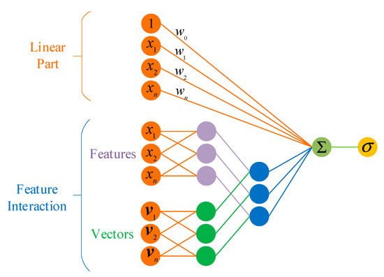
Figure 1. Factorization machine.

This is similar to matrix decomposition in collaborative filtering, and the expression of an FM is

$$\widehat{y}\left(\mathit{x}\right)=\sigma \left(w_0+{\displaystyle \sum _{i=1}^N{w}_i{x}_i}+{\displaystyle \sum _{i=1}^{N-1}{\displaystyle \sum _{j=i+1}^N<{\mathit{v}}_i,{\mathit{v}}_j>x_i{x}_j}}\right)$$

(5)

where ${\mathit{v}}_i$ represents the latent vector of feature component $x_i$, whose length is $K$ ($K\in N^{+},K<<N$); $<\cdot ,\cdot >$ represents the dot product; $N$ is the number of features; $w_0\in R$, and $\mathit{w}=\{w_1,w_2,\cdot \cdot \cdot ,w_n\}\in R^N$. The sigmoid function is set on the output of the FM so the model output will be converted between 0 and 1.

All feature interactions containing feature $x_i$ have the opportunity to learn the latent vector ${\mathit{v}}_i$. This advantage enables the FM to cope well with high-dimensional sparse data and less-relative samples. According to the perfect square trinomial, Equation (5) is transformed as follows:

$$\widehat{y}\left(\mathit{x}\right)=\sigma \left(w_0+{\displaystyle \sum _{i=1}^N{w}_i{x}_i}+\frac{1}{2}{\displaystyle \sum _{k=1}^K\left[{\left({\displaystyle \sum _{i=1}^N{v}_{i,k}{x}_i}\right)}^2-{\displaystyle \sum _{i=1}^N{v}^2{}_{i,k}{x}_i{}^2}\right]}\right)$$

(6)

The time complexity of the model changed from $O\left(K{N}^2\right)$ to $O\left(KN\right)$. Based on logistic regression, the FM models the interaction between features and proposes the latent vector to estimate the model. Thus, it can be seen that an FM can complete the target task in linear time. The stochastic gradient descent (SGD) method was used to learn the FM parameters, as shown in Algorithm 1.

Algorithm 1: SGD optimizes FM.

Input: dataset $D=\{{\mathit{x}}_m,y_m{\}}_{m=1}^M,\mathit{x}\in R^N,y\in R$ Output: model parameters ${\theta }^{*}=\{w_0,\mathit{w},V\}$ Initialize: $\alpha =0.1,w_0=0,\mathit{w}=\mathbf{0},V\to N(0,1)$ $\mathrm{for}\hspace{0.17em}m=1\cdot \cdot \cdot M\hspace{0.17em}\mathrm{do}$ $\widehat{y}\left({\mathit{x}}_m\right)=\sigma \left(w_0+{\displaystyle \sum _{i=1}^N{w}_i{x}_i}+{\displaystyle \sum _{i=1}^{N-1}{\displaystyle \sum _{j=i+1}^N<{\mathit{v}}_i,{\mathit{v}}_j>x_i{x}_j}}\right)$ $w_0\leftarrow w_0-\alpha \frac{\partial }{\partial w_0}loss\left({\widehat{y}}_m\left({\mathit{x}}_m|{\theta }^{*}\right),y_m\right)$ $\mathrm{for}\hspace{0.17em}i=1\cdot \cdot \cdot N\hspace{0.17em}\mathrm{do}$ $w_i\leftarrow w_i-\alpha \frac{\partial }{\partial w_i}loss\left({\widehat{y}}_m\left({\mathit{x}}_m|{\theta }^{*}\right),y_m\right)$ $\mathrm{for}\hspace{0.17em}k=1\cdot \cdot \cdot K\hspace{0.17em}\mathrm{do}$ $v_{ik}\leftarrow v_{ik}-\alpha \frac{\partial }{\partial v_{ik}}loss\left({\widehat{y}}_m\left({\mathit{x}}_m|{\theta }^{*}\right),y_m\right)$ $\mathrm{end}$ $\mathrm{end}$ $\mathrm{end}$

2.3. Cascade Model

The training process of XGBoost can be regarded as the combination of the single feature of each decision tree. Generally, the combined features are better than the original features; hence, the new features transformed by XGBoost also have strong information capacities.

Assuming that the feature set of the dataset is $C=\left\{c_1,c_2,\cdots c_N\right\}$, a sample can be expressed as ${\mathit{x}}_{\mathrm{i}}=\left\{x_1,x_2,\cdots x_N\right\}$, ${\mathit{x}}_i\in R^N$. The function of XGBoost is to map a sample to the leaf node of each subtree to obtain the index vector corresponding to the sample:

$$\mathrm{X}\mathrm{G}\mathrm{B}\mathrm{o}\mathrm{o}\mathrm{s}\mathrm{t}:\hspace{1em}{\mathit{x}}_i\to {\mathit{\omega }}_i$$

(7)

where ${\mathit{\omega }}_i=\left\{{\omega }_{i1},{\omega }_{i2},\cdots {\omega }_{iT}\right\}$ and $T$ is the number of decision trees. Equation (7) is the key to feature transformation. Element ${\omega }_{ik}$ in ${\mathit{\omega }}_i$ encodes the node, where sample ${\mathit{x}}_i$ maps to the kth subtree. Vector ${\mathit{\omega }}_i$ is regarded as the feature vector of the original sample transformed by XGBoost. ${\mathit{\omega }}_i$ is a new feature vector of the implicit information of the original sample ${\mathit{x}}_i$, and the result of its one-hot encoding is ${\tilde{\mathit{\omega }}}_i$. At this time, element ${\tilde{\mathit{\omega }}}_{ik}$ in ${\tilde{\mathit{\omega }}}_i$ is a sparse vector of length $l_k$. The position element corresponding to ${\omega }_{ik}$ in ${\tilde{\mathit{\omega }}}_{ik}$ is 1, and the other position elements are 0. Therefore, the dimension of the new vector ${\tilde{\mathit{\omega }}}_i$ transformed by XGBoost is the sum of the leaf nodes of all subtrees $N^{\prime }={\displaystyle {\sum }_{k=1}^T{l}_k}$.

Although $N^{\prime }>>N$, transformed high-dimensional sparse vectors do not increase the computational cost of FM model training but make the interaction part of the model easier to carry out.

For a trained XGBoost model (See Figure 2), suppose that the leaf nodes of the kth tree are coded from left to right according to natural numbers, which are recorded as

$$L_k=\left\{1,2,\cdots l_k\right\},k\in T$$

(8)

where $l_k$ is the number of leaf nodes in the current subtree. Assume $C_k(C_k\subset C)$ is the feature set used to build the kth tree, which is equivalent to selecting a feature set for the current subtree. Due to the limitation of the decision tree depth, XGBoost only uses a small part of the features when constructing a subtree, so $l_k$ and $C_k$ are generally small, which is helpful for accelerating model training and preventing overfitting.

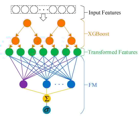
Figure 2. Extreme gradient boosting (XGBoost) and factorization machine (XGB+FM) cascade model.

3. Data

Two data sources were used in this study. The time resolution of the first part of the data was 1 h, which was used to capture ground information. Att-Bi-LSTM was proposed to solve the missing values of the data. The time resolution of the second part of the data was 8 h, which was used to capture high-altitude information. In order to forecast the severe convective weather in Tianjin, the latest data of the two datasets before the occurrence of the target weather were integrated. In view of the imbalance of hail and rainstorm samples, a new oversampling algorithm was proposed to synthesize the hail samples.

3.1. Dataset

The dataset came from the automatic meteorological station of Tianjin and its surrounding weather system moving path radiosonde station, and its geographical distribution is shown in Figure 3.

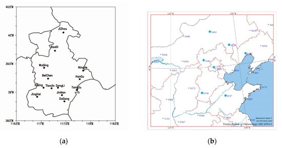
Figure 3. Sources of meteorological data in Tianjin: (a) distribution of automatic meteorological stations in Tianjin and (b) distribution of radiosonde stations around Tianjin.

As shown in Figure 3a, there are 13 automatic meteorological observation stations in Tianjin, and the observation data records 20 meteorological physical quantities with a temporal resolution of 1 h, which can be found in Appendix A. According to the geographical location of Tianjin City in Figure 3b, Beijing Station and Zhangjiakou Station on Northwest Road, Chifeng Station on Northeast Road, Xingtai Station on Southwest Road and Zhangqiu Station on Southeast Road were selected as the auxiliary for the forecast of heavy rain and hail in the Tianjin area. Each radiosonde station calculated 33 convection parameters based on the physical quantity. Detailed information can be found in Appendix B. Table 1 is the individual station information in Figure 3b.

Table 1. Radiosonde station information.

Station	Station Number	Longitude	Latitude	Altitude
Beijing	54451	116.4667	39.8	31.3
Xingtai	53798	114.3589	37.1808	183
Zhangqiu	54727	117.55	36.6833	121.8
Chifeng	54218	118.8344	42.3075	668.6
Zhangjiakou	54401	119.9194	40.7694	772.8

3.2. Missing Data Imputation

The data recorded by the automatic station (Appendix A) was collected on an hourly basis, and we selected the measured data from 2006 to 2018. However, there were missing values in the data of the automatic observation station, which occurred only in the first through the tenth physical quantities. Statistics show that about 40 data values were not recorded each year on average. Missing meteorological values is the most common issue in statistical analysis and the most important way to improve the reliability of analysis results, mainly caused by extreme weather conditions and various mechanical failures [24]. Meteorological data has strict spatial and temporal correlation, and a method that can not only guarantee the accuracy of meteorological data, but also impute the missing values of data in real time, must be used. We used a Bi-LSTM model that introduced an attention mechanism to impute missing values. The input of Att-Bi-LSTM was ten physical quantities in the first three hours, and the prediction was ten physical quantities in the next moment, which could be used for estimating the missing data values.

Compared with Recurrent Neural Network (RNN), LSTM introduces a new memory cell ${\mathit{c}}_t\in {ℝ}^D$ to store the experience learned from historical information and retain the captured information for a longer time interval. Memory cell ${\mathit{c}}_t$ is calculated by the following formula:

$${\mathit{c}}_t={\mathit{f}}_t\odot {\mathit{c}}_{t-1}+{\mathit{i}}_t\odot {\tilde{\mathit{c}}}_t$$

(9)

$${\mathit{h}}_t={\mathit{o}}_t\odot \tanh ({\mathit{c}}_t)$$

(10)

where ${\mathit{f}}_t\in {[0,1]}^D$, ${\mathit{i}}_t\in {[0,1]}^D$ and ${\mathit{o}}_t\in {[0,1]}^D$ are the three gates that control the information transmission path; $\odot$ is the product of the vector elements; ${\mathit{c}}_{t-1}$ is the memory unit at time $t-1$; and ${\tilde{\mathit{c}}}_t\in {ℝ}^D$ is the current candidate state, obtained through the following nonlinear function:

$${\tilde{\mathit{c}}}_t=\tanh ({\mathit{W}}_c{\mathit{x}}_t+{\mathit{U}}_c{\mathit{h}}_{t-1}+{\mathit{b}}_c)$$

(11)

where ${\mathit{x}}_t$ is the input data at the current moment and ${\mathit{h}}_{t-1}$ is the external input of the previous moment.

LSTM connects two memory cells through a linear relationship, which is more than effective for solving the vanishing gradient problem [25]. The gating mechanism in LSTM is actually a kind of soft threshold gate with a value between 0 and 1, indicating the proportion of information allowed to pass, as shown in Figure 4.

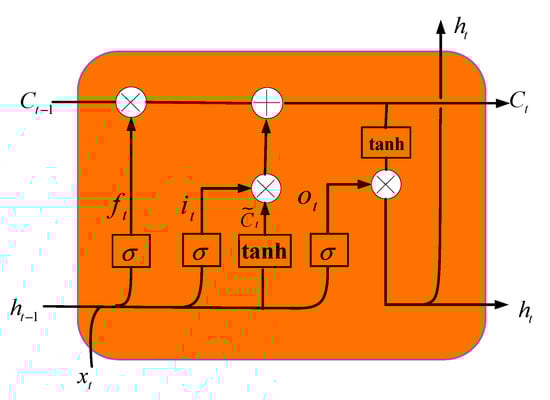
Figure 4. Structure of a long short-term memory (LSTM) network unit.

The bidirectional LSTM network adds a network layer that transmits information in reverse order to learn more advanced features, which allows the LSTM network to operate in two ways: one from the past to the future and the other from the future to the past. Specifically, the bidirectional LSTM can store information from past and future moments in two hidden states at any time. Assuming that the hidden states of the LSTM network in two opposite directions at time $t$ are ${\mathit{h}}_t^1$ and ${\mathit{h}}_t^2$, then

$${\mathit{h}}_t^1=f({\mathit{W}}^1{\mathit{x}}_t+{\mathit{U}}^1{\mathit{h}}_{t-1}+{\mathit{b}}^1)$$

(12)

$${\mathit{h}}_t^2=f({\mathit{W}}^2{\mathit{x}}_t+{\mathit{U}}^2{\mathit{h}}_{t+1}+{\mathit{b}}^2)$$

(13)

$${\mathit{h}}_t={\mathit{h}}_t^1\oplus {\mathit{h}}_t^2$$

(14)

where $\oplus$ represents the vector splicing operation and ${\mathit{h}}_t$ is the output at time t.

An attention mechanism is an effective means to tackle information overload [26]. The purpose of an attention mechanism is to save computing resources, strengthen the capacity and expression performance of the network and filter the information irrelevant to the task for the neural network, inspired by the mechanisms of the human brain.

Let $\mathit{H}=[{\mathit{h}}_1,{\mathit{h}}_2,\cdots ,{\mathit{h}}_T]\in {ℝ}^{D\times T}$ be the output of the bidirectional LSTM network, where $T$ is the sequence length and $D$ is the dimension of the output vector. In Att-Bi-LSTM, the query vector $\mathit{q}$ is dynamically generated, and the final state ${\mathit{h}}_T$ learned by each sequence is defined as $\mathit{q}$. At this time, the network is considered to have learned the most beneficial information for the task. The scaled dot product model is regarded as a metric to indicate the similarity of vectors $\mathit{q}$ and $\mathit{h}$:

$$s(\mathit{h},\mathit{q})=\frac{{\mathit{h}}^T\mathit{q}}{\sqrt{D}}$$

(15)

Equation (15) is called the scoring function of attention. Therefore, when $\mathit{q}$ and $\mathit{h}$ are given, the probability of the tth input vector being selected is

$$\begin{array}{l}{\alpha }_t=p(t|\mathit{H},\mathit{q})\\ \hspace{1em}\hspace{0.17em}=\mathrm{softmax}\left(s({\mathit{h}}_t,\mathit{q})\right)\\ \hspace{1em}\hspace{0.17em}=\frac{\exp \left(s({\mathit{h}}_t,\mathit{q})\right)}{{\displaystyle {\sum }_{i=1}^T\exp \left(s({\mathit{h}}_i,\mathit{q})\right)}}\end{array}$$

(16)

where ${\alpha }_t$ is the attention distribution of the model, indicating the degree of attention paid to the tth input vector. As shown in Figure 5, the soft attention mechanism is the weighted average of the output vectors at all times:

$$att(\mathit{H},\mathit{q})={\displaystyle {\sum }_{t=1}^T{\alpha }_t}{\mathit{h}}_t$$

(17)

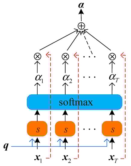
Figure 5. Soft attention mechanism.

With the help of the attention mechanism, the LSTM network can capture important semantic information in the data. Therefore, the proposed model can automatically give priority to the expressions that are beneficial to the prediction results without using external information. As shown in Figure 6, the model of missing data imputation consisted of five parts, and we sorted out the data in the preprocessing layer, mainly including normalization. Table 2 and Figure 7 show the goodness of fit and partial visualization of Att-Bi-LSTM to meteorological physical quantities, respectively, which prove that the model used to estimate missing data is reliable. The best values are indicated in bold in the table. In practical application, the data of the three moments before the occurrence of missing values is modeled, and the hourly predictions of multiple features are obtained to estimate the missing value.

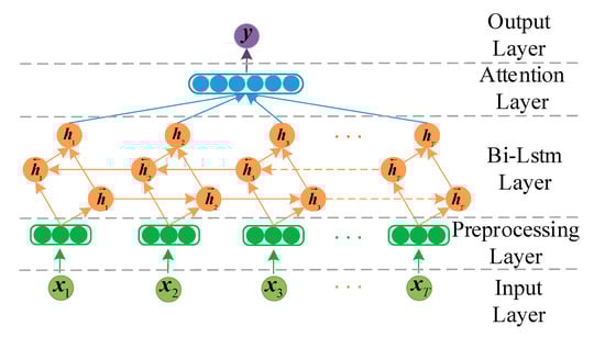
Figure 6. Structure of attention-based bidirectional long short-term memory (Att-Bi-LSTM).

Table 2. Goodness of fit of the physical quantity.

${\mathit{R}}^{\mathbf{2}}$	PRS	PRS_Sea	TEM	DPT	RHU	VAP	WIN_D_2mi	WIN_S_2mi	WIN_D_10mi	WIN_S_10mi
LSTM	0.9766	0.9764	0.9403	0.9564	0.9432	0.9566	0.3317	0.50660	0.3623	0.5970
Bi-LSTM	0.9981	0.9982	0.9964	0.9972	0.9980	0.9987	0.9881	0.9909	0.9870	0.9930
Att-Bi-LSTM	0.9961	0.9963	0.9973	0.9988	0.9985	0.9990	0.9888	0.9942	0.9880	0.9945

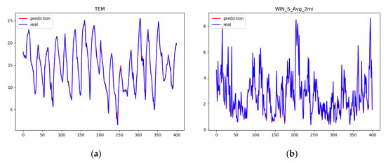
Figure 7. Partial visualization of the physical quantities for (a) temperature and (b) average wind speed in 2 min.

3.3. Data Integration

Meteorological observatory data were recorded hourly in Coordinated Universal Time (UTC) and converted to Chinese standard time. According to the occurrence of heavy precipitation and hail in Tianjin, the meteorological physical quantity three hours before the occurrence time (OT) was obtained, with a total of 60 features. The radiosonde data was recorded twice a day at 8:00 a.m. and 8:00 p.m. Chinese standard time, respectively. The data of five radiosonde stations were obtained from the previous detection at the OT with a total of 165 features. Finally, the two datasets (Appendix A and Appendix B) were merged according to the OT, and the forecast datasets of heavy precipitation and hail were obtained. Thus, the final dataset had 225 features, and the labels were based on the heavy precipitation and hail recorded by the automatic observation stations. In addition, weather categories not covered in this research were excluded by the Tianjin rainfall forecast system. This paper integrates the data from the above two sources to build a regional forecast system.

3.4. Class Imbalance

The traditional SMOTE algorithm adopts a random linear interpolation strategy, and the synthesized sample will attract the hyperplane to move to the minority class. However, this random strategy cannot influence the distance of the hyperplane movement. When the dataset is extremely unbalanced, the synthesized samples are likely to overlap with the original data and even introduce noise samples, which leads to problems such as fuzzy hyperplanes and the marginalization of data distribution [27].

The oversampling algorithm-based support vector was proposed by Wang in 2007 [28], which performs near-neighbor extensions on minority class support vectors instead of minority classes. The innovation of this study was to propose two interpolation methods based on the support vector decision mechanism. First, we used the SVM algorithm to find the support vector, namely the two types of samples in the dataset located at the decision boundary. Second, a discrimination strategy for the sample was applied to the support vectors belonging to a minority class. Finally, two different interpolation methods were introduced according to the characteristics of support vector: sample interpolation and sample extrapolation.

The SVM-SMOTE algorithm is as follows:

• SVM is used to find all the support vectors in the minority class;
• For each support vector $\mathit{x}$ of the minority class, the $k$ nearest neighbors are calculated according to Euclidean distance, assuming that the number of majority classes in $k$ nearest neighbors is $n$. If $n=k$, $\mathit{x}$ is marked as noise; if $n>k/2$, $\mathit{x}$ is marked as danger; and if $n<k/2$, $\mathit{x}$ is marked as safety, as shown in Figure 8;
  

  Figure 8. Support vector machines–synthetic minority oversampling technique (SVM-SMOTE) oversampling algorithm’s (a) sample discrimination mechanism and (b) method of sample interpolation and sample extrapolation. (Orange dots indicate the majority class, and blue stars indicate the minority class).
• For each danger ${\mathit{x}}_i$, the minority sample ${\mathit{x}}_j$ of the $k$ nearest neighbors is found, and the sample interpolation method is adopted to synthesize new minority samples between them:

  $${\mathit{x}}_{new}={\mathit{x}}_i+rand(0,1)*({\mathit{x}}_j-{\mathit{x}}_i)$$

  (18)
• For each safety ${\mathit{x}}_i$, the sample extrapolation method is

  $${\mathit{x}}_{new}={\mathit{x}}_i-rand(0,1)*({\mathit{x}}_j-{\mathit{x}}_i)$$

  (19)

  where $rand(0,1)$ is a random number between 0 and 1.

The essence of SVM-SMOTE is to synthesize samples with different discrimination mechanisms for minority support vectors. This algorithm can extend the minority class to the sample space with a low majority class density, which is beneficial to subsequent classification tasks. In the data preprocessing stage, this research used SVM-SMOTE to synthesize hail samples so as to reduce the class imbalance. Specifically, the number ratio of heavy precipitation to hail was closer to 7:1. After SVM-SMOTE algorithm processing, the hail samples in the train set were expanded from 50 to 332, which made the number of the two classes equal.

4. Experiment

At the end of data preprocessing, the XGB+FM model proposed in this paper was formally applied. Because the hyperparameters were difficult to interpret, we adopted Bayesian optimization to fine-tune the model. In view of many meteorological elements, the proposed method for selecting factors was proven to be effective.

4.1. Hyperparameter Optimization

The hyperparameter tuning of machine learning models could be regarded as an optimization process of black box functions [29]. For computational reasons, the cost of optimizing this function was high, and more importantly, the expression of the optimized function was unknown. Bayesian optimization provided new ideas for the global optimization of such models.

In this paper, we used the Bayesian optimization algorithm based on a Gaussian process to achieve the hyperparameter tuning of XGBoost [30]. Assuming that the search space of the hyperparameters is represented as $X$, and the black box function can be defined as $f:\mathit{x}\to R$, the goal of optimization is to find suitable parameter values to satisfy

$${\mathit{x}}^{*}=\underset{x\in X}{\arg \max }f(\mathit{x})$$

(20)

For ease of presentation, the input samples were omitted here, and $\mathit{x}$ represents a set of hyperparameters to be optimized. Through the Gaussian process, Bayesian optimization could statistically obtain the mean and variance of all hyperparameters corresponding to the current iteration number. A larger mean was expected by the model, and variance represented the uncertainty of the hyperparameters.

In Figure 9, the solid green line represents the empirical error as a function of the hyperparameters, the orange area represents the variance, the green dashed line represents the mean and the red dot is the empirical error, calculated based on the three sets of hyperparameters of the model. In order to find the next set of optimal hyperparameters, the model should comprehensively consider the mean and variance and define the acquisition function for

$$\partial (t)={\mu }_{t-1}(\mathit{x})+{\beta }_t^{\raisebox{1ex}{$1$}\!\left/ \!\raisebox{-1ex}{$2$}\right.}{\sigma }_{t-1}(\mathit{x})$$

(21)

where ${\mu }_{t-1}(\mathit{x})$ and ${\sigma }_{t-1}(\mathit{x})$ represent the mean and variance of the previous iteration. ${\beta }_t$, according to theoretical analysis, generally increases with the number of iterations.

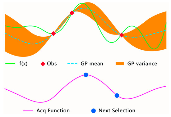
Figure 9. Bayesian optimization based on a Gaussian process.

The acquisition function was used to calculate the weighted sum of the mean and the variance, as shown by the purple solid line in Figure 9. The algorithm needed to find the maximum value and add it to the historical results to recalculate the two parameters of the Gaussian process. The details of the implementation can be seen in Algorithm 2.

Algorithm 2: Bayesian optimization.

Input: dataset $D_0$, Number of iterations $T$ Output: ${\mathit{x}}_{\max }$, $y_{\max }$ Initialize: $\alpha =0.1,w_0=0,\mathit{w}=\mathbf{0},V\to N(0,1)$ $\mathrm{for}\hspace{0.17em}t=1\cdot \cdot \cdot T\hspace{0.17em}\mathrm{do}$

Fit GP according to data set $D_0$, ${\mathit{x}}_t=\arg \max \partial (\mathit{x})$

Evaluate $y=f({\mathit{x}}_t)$, $D_t=D_{t-1}\cup \left({\mathit{x}}_t,y_t\right)$

$\mathrm{end}$

This paper used Bayesian optimization to tune eight hyperparameters of XGBoost, and the results are shown in Figure 10. Based on the optimization results, the selected hyperparameter combinations are shown in Table 3 and Table 4.

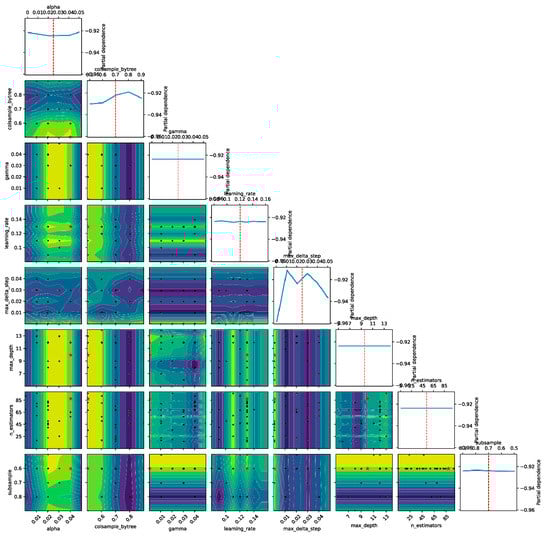
Figure 10. The result of Bayesian optimization. (The red dotted line represents the mean of the candidate values. The blue line represents the score of each parameter on the candidate value).

Table 3. Hyperparameters of XGBoost.

Hyperparameter	Explanation	Value
alpha	L1 regularization	0.01
colsample_bytree	Subsample ratio of columns when constructing each tree	0.9
gamma	Minimum gain of node split	0.05
learning_rate	Boosting learning rate	0.12
max_delta_step	Maximum delta step for tree weight change	0
max_depth	Maximum tree depth for base learners	6
n_estimators	Number of trees	60
subsample	Subsample ratio of the training instance	0.6

Table 4. Hyperparameters of the FM.

Hyperparameter	Explanation	Value
lr	L2 regularization	0.15
lambda	Regularization	0.04
epoch	Number of iterations	30
k	Latent vector length	4

4.2. Evaluation

In this paper, three evaluation indicators commonly used in severe convection forecasting and receiver operating characteristic (ROC) curves were used to measure the performance of different models. The area-under-the-curve (AUC) value was not affected by the size of the test data, and it was expected for the classifier to find an appropriate threshold for both the positive and negative classes:

$$\mathrm{A}\mathrm{U}\mathrm{C}={\displaystyle {\sum }_{i\in (P+N)}\frac{(TP{R}_i+TP{R}_{i-1})(FP{R}_i-FP{R}_{i-1})}{2}}$$

(22)

The commonly used assessment indicators in the meteorological field were the percent of doom (POD), false alarm rate (FAR) and threat score (TS). With the help of the confusion matrix (See Table 5), the above three indicators (with hail as the object of concern) can be better expressed as

$$\mathrm{P}\mathrm{O}\mathrm{D}=\frac{TP}{TP+FN}$$

(23)

$$\mathrm{F}\mathrm{A}\mathrm{R}=\frac{FP}{TP+FP}$$

(24)

$$\mathrm{T}\mathrm{S}=\frac{TP}{TP+FP+FN}$$

(25)

Table 5. The confusion matrix.

Real Class	Forecast Class
	Hail	Heavy Precipitation
Hail	$TP$	$FN$
Heavy precipitation	$FP$	$TN$

In this paper, 82 cases of heavy rainfall and hail in Tianjin in the past 12 years were forecasted, and various ensemble learning strategies and corresponding cascade models were compared. In view of the unbalanced test set, in order to increase the credibility of the experimental results, all comparison experiments were tested four times. The average results are shown in Table 6. The error bars of the four performances of XGB+FM can be seen in Figure 11a.

Table 6. The results of the experiment.

Mode	POD	FAR	TS
RF	0.5910	0.5336	0.3512
GBDT	0.5455	0.5885	0.3333
XGBoost	0.6364	0.5625	0.3500
RF+LR	0.6591	0.4917	0.4018
GBDT+LR	0.7046	0.5230	0.3974
XGB+LR	0.7500	0.5344	0.4034
XGB+FM	0.9318	0.5054	0.4761

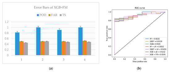
Figure 11. The experimental results’ (a) error bars and (b) receiver operating characteristic (ROC) curve.

Figure 11b is an ROC curve of the experimental results. Up to now, this paper proposed XGBoost as a feature engineering approach which selected important features and tried to transform them, and an FM was used as the model of the classifier. As shown in Table 6 and Figure 11, compared with other cascading strategies, XGB+ FM had the best AUC value and the best performance for the POD and TS, the latter of which is more concerned with severe convection prediction. However, the FAR of our model was slightly behind RF+LR and ranked second.

4.3. Feature Importance

In analyzing the experimental results of the previous section, although the RF had a low POD of hail, the POD of heavy rain was relatively high, which made its AUC value larger. As a bagging ensemble learning method, a RF adopts the strategy of random selection of feature subsets in tree construction, which can indeed improve the results. All the features involved in this paper are commonly used forecast factors in the field of meteorology, and the selection of meteorological factors is a part of the work that is exceedingly concerned with weather forecasting. Therefore, this section attempts to illustrate forecast factors based on the above work.

The importance of features is an essential factor affecting the forecast performance and efficiency, and the most important feature expression model was expected. Another hidden function of XGBoost is that it can assign a score to each feature based on the set of established decision trees, which indicates the contribution of the feature to the boosting tree [31]. Three commonly used feature description methods in boosting ensemble learning are weight, gain, and cover [32]. Weight is the number of times each feature is used in the model; gain is the average gain of splits which use the feature; and cover is defined as the average number of samples affected by the feature splitting. Based on the above three indicators, the 30 most important features of XGBoost and their quantitative relationships are shown in Figure 12.

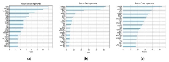
Figure 12. Feature importance of (a) weight, (b) gain and (c) cover.

However, it can be seen from the figure that the three methods were inconsistent in describing the importance of features, as they only showed the relative importance of different factors but did not reflect the contribution of forecast factors to forecast accuracy.

The number of features was another factor weighing predictive performance against efficiency. In order to illustrate the features better, we first got a contribution value for each feature. Secondly, with reference to boosting feature importance [33], the goal was to get the cumulative contribution degree caused by the features. Finally, after the feature contributions were arranged in descending order, a factor cumulative contribution diagram was obtained, as shown in Figure 13.

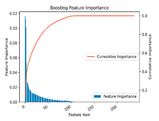
Figure 13. Boosting feature importance.

Generally speaking, a small number of features dominated the contribution values, while other features did not provide or rarely provided contributions. In Figure 13, we see the expected results. The top 50 features were 80% important to the model, and the top 100 features contributed almost 100% to the importance of the features. Moreover, the first four features were significantly more explanatory than the other features, while the last 200 features did not provide any explanatory ability for the model. Therefore, a more effective method to describe the importance of features was urgently needed for the selection of meteorological factors.

4.4. Factor Selection

In the field of meteorology, the selection of factors is of great importance to the accuracy of forecasts. Traditional methods for the selection of meteorological factors include the variance method and correlation coefficient method [34]. However, many factor selection methods fail to take into account the influence of correlation information between factors on the accuracy of forecasts.

It is worth mentioning that the feature interaction of the FM model provides a new idea for selecting the optimal combination of features. Given that the dimension of the new sample ${\tilde{\mathit{\omega }}}_i$ transformed by XGBoost is $N^{\prime }$, the second-order FM model of the transformed sample can be obtained according to Equation (5):

$$\widehat{y}\left({\tilde{\mathit{\omega }}}_i\right)=\sigma \left({\lambda }_0+{\displaystyle \sum _{j=1}^{N^{\prime }}{\lambda }_j{\tilde{\omega }}_{i,j}}+{\displaystyle \sum _{j=1}^{N^{\prime }-1}{\displaystyle \sum _{k=j+1}^{N^{\prime }}<{\mathit{v}}_j,{\mathit{v}}_k>{\tilde{\omega }}_{i,j}{\tilde{\omega }}_{i,k}}}\right)$$

(26)

where ${\tilde{\omega }}_{i,j}$ is the jth feature of the ith transformed sample ${\tilde{\mathit{\omega }}}_i$ and its value is either zero or one. Different from the above experimental part, when using the interactive characteristics of the FM model to select the optimal combination feature, attention should be paid to the second-order polynomial part of the model, according to the following definition:

$${\lambda }_{jk}=<{\mathit{v}}_j,{\mathit{v}}_k>$$

(27)

where ${\lambda }_{jk}$ is the second-order polynomial coefficient of the model, which represents the contribution degree of the feature combinations ${\tilde{\omega }}_{i,j}$ and ${\tilde{\omega }}_{i,k}$ to the model. The factor threshold $\epsilon$ is set here, and the feature combinations ${\tilde{\omega }}_{i,j}$ and ${\tilde{\omega }}_{i,k}$, corresponding to ${\lambda }_{jk}>\epsilon$, are selected; that is, the combined features whose contribution degrees are greater than $\epsilon$ are considered to be important factors.

Assuming that the set of coefficients satisfying the above conditions is $\lambda =\{{\lambda }_{jk}|{\lambda }_{jk}>\epsilon \}$, for ${\lambda }_{jk}$, it must correspond to the transformed features ${\tilde{\omega }}_{i,j}$ and ${\tilde{\omega }}_{i,k}$ of the two subtrees. Let the set used by XGBoost to construct these two subtrees be $C_j$ and $C_k$. Then, the optimal feature combination can be expressed as $C_j\cup C_k$. Take the intersection of all the feature combinations that meet the above threshold conditions, and the feature with greater contribution selected by the FM can be expressed as

$$\tilde{C}={\cup }_{j,k\in \lambda }\left(C_j\cup C_k\right)$$

(28)

where $\tilde{C}$ is the optimal feature set selected by the FM second-order coefficients. In this paper, the linear term coefficients of the FM model were also selected.

4.5. Results and Discussion

The feature score endows each feature with a numerical weighted feature importance (WFI). In this paper, the XGBooost program (See Figure 14) was executed based on the selected feature subset of the given WFI threshold. The opinion here is that, after the XGBoost system performed feature selection, we used it to capture higher-order feature interactions that captured orders one less than the depth of the decision tree. The order in which the decision tree was built determined the order of feature interactions.

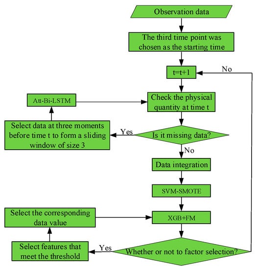
Figure 14. System function diagram.

In this section, 60 decision trees (See Figure 15) established in Section 4.1 were used to transform features, and a total of 341 dimension features were obtained, which corresponded to 341 feature latent vectors. According to Equations (27) and (28), the optimal factor combination was calculated and selected. In addition, improvements in the experimental results were compared between the traditional factor selection method and the XGBoost factor selection method.

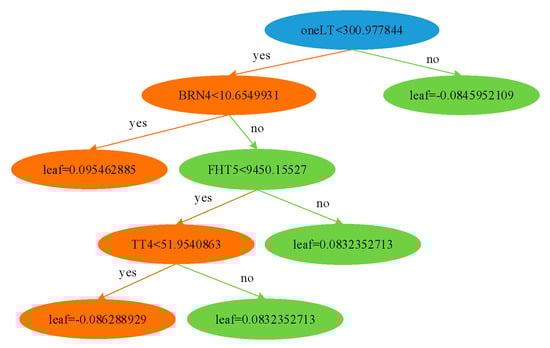
Figure 15. A subtree of XGBoost.

Table 7 shows the thresholds and results corresponding to the three feature selection methods. This paper did not use a recursive method to find the optimal threshold, which was not the focus of this work.

Table 7. Feature selection.

Method	Threshold	Number of Features
Correlation coefficient [34]	0.2	67
XGBoost [31]	0.001	99
XGB+FM	0.02	82

We re-executed the XGB+FM model with the results of feature selection, and the experimental results and ROC curves of the three feature selection methods are shown in Table 8 and Figure 16.

Table 8. Experimental results of feature selection.

Method	POD	FAR	TS
Correlation coefficient [34]	1.0	0.5417	0.4583
XGBoost [31]	0.9091	0.4118	0.5555
XGB+FM	1.0	0.4211	0.5789

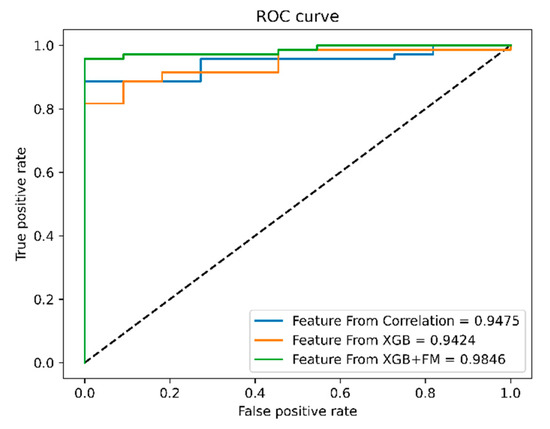
Figure 16. ROC curve after feature selection. (The black line represents the result of random guessing.)

As can be seen from the results, compared with the other two methods, the model after XGB+FM factor selection was more efficient. XGB+FM factor selection was superior to the other two methods in terms of TS, which attracted more attention. The POD was equal to the correlation coefficient method. Meanwhile, the three indicators of our method were better than the forecast results without factor selection. However, the consequence was not exceedingly satisfactory. Eight of the 71 heavy precipitation cases were still expected to be hail. In addition to the imbalance of the test set, another potential contributor for this result may be that the train set still did not support the model to get a better parameter space, which is also urgent work for the future.

The factor selection method proposed in this paper is reasonable. The process of XGBoost tree construction ensures the effectiveness of factors, and the FM model considers the correlation among the factors and finds the optimal combination of factors to achieve more exciting forecast results. In practical application, the proposed method can significantly reduce the storage space and model training time of meteorological big data and promote forecast performance at an appropriate threshold.

In general, the following results can be seen. Adding feature interaction on the basis of linear features was helpful to improve the forecast accuracy. Learning of both low-order (FM) and high-order (XGBoost) features improved the reliability of the forecast results. The forecast results were improved based on the important features selected by XGB+FM. Finally, the performance of the model could be improved through feature interaction.

5. Conclusions

In this paper, the difficulties of severe convective weather region forecast were solved. A severe convection forecast method was proposed, in which XGBoost and the FM model were cascaded to improve the forecast accuracy. We suggested a bidirectional LSTM network with the attention mechanism to impute missing data. We put forward an SVM-SMOTE algorithm to overcome the problem of long-tailed data distributions. Meanwhile, a Bayesian optimization algorithm was adopted to fine-tune the hyperparameters of the model. Our experiment results demonstrate the following:

• The SVM-SMOTE algorithm innovatively proposed two interpolation methods based on a sample discrimination mechanism, and the consequence showed the effectiveness of the discrimination based on the boundary area. The main advantages are that support vectors are often partial samples of minority classes, which reduces the time complexity, and support vectors are bounded, which may increase the classification ability of the dataset;
• In our model, the transformed features of XGBoost are sparse, which can reduce the influence of noisy data and improve the robustness of the hybrid model. As a probabilistic nonlinear classifier, the FM’s interactive feature function is more than effective for sparse features and helps to capture the nonlinear interaction between features;
• XGB+FM learns both low-order and high-order features at the same time to improve forecast accuracy, which is important to attempt in the field of meteorology.

In view of the large number of forecast factors in the meteorological field, a forecast factor selection technique was proposed to strengthen forecast performance. By analyzing feature importance, the results of the machine learning models are easier to understand:

• This study proves that both the number of decision trees and the number of features affect the forecast results. Therefore, more important features need to be selected for severe convection forecasting;
• XGB+FM proposes a new evaluation method for feature importance, which greatly reduces the learning time by discarding features with low correlation and, at the same time, alleviating the storage consumption of meteorological big data;
• XGB+FM is more powerful after factor selection than other ensemble strategies. Meteorologists can then decide which factors to refeed into the model for better results.

Limited by the number of severe convective weather and the diversity of features, our model may not be able to maximize the forecast advantage. Another possible model training method is to train the feature engineering XGBoost model with part of the data set and train the FM classifier with another part of the data. In actual situations, the dataset should be updated continuously, according to climate change, to improve the performance of severe convection forecasting. Our research proves the effectiveness of high-altitude factors for forecasting severe convection. However, the difference of meteorological factors toward the formation mechanism of heavy precipitation and hail is still worthy of further study. Future work can also study the interaction between XGBoost and FMs. As an example, XGBoost can be trained with meteorological data for one season, while the parameters of an FM can be trained once a week—or otherwise once a month—which may be more consistent with the seasonal characteristics of meteorological data.

References

- Hand, W.H.; Cappelluti, G. A Global Hail Climatology Using the UK Met Office Convection Diagnosis Procedure (CDP) and Model Analyses: Global Hail Climatology. Meteorol. Appl. 2011, 18, 446–458. [Google Scholar] [CrossRef]
- Brimelow, J.C.; Burrows, W.R.; Hanesiak, J.M. The Changing Hail Threat over North America in Response to Anthropogenic Climate Change. Nat. Clim. Chang. 2017, 7, 516–522. [Google Scholar] [CrossRef]
- Hao, W.; Hao, Z.; Yuan, F.; Ju, Q.; Hao, J. Regional Frequency Analysis of Precipitation Extremes and Its Spatio-Temporal Patterns in the Hanjiang River Basin, China. Atmosphere 2019, 10, 130. [Google Scholar] [CrossRef]
- Moura Cardoso do Vale, T.; Helena Constantino Spyrides, M.; De Melo Barbosa Andrade, L.; Guedes Bezerra, B.; Evangelista da Silva, P. Subsistence Agriculture Productivity and Climate Extreme Events. Atmosphere 2020, 11, 1287. [Google Scholar] [CrossRef]
- Kunz, M.; Wandel, J.; Fluck, E.; Baumstark, S.; Mohr, S.; Schemm, S. Ambient Conditions Prevailing during Hail Events in Central Europe. Nat. Hazards Earth Syst. Sci. 2020, 20, 1867–1887. [Google Scholar] [CrossRef]
- Manzato, A. Hail in Northeast Italy: Climatology and Bivariate Analysis with the Sounding-Derived Indices. J. Appl. Meteorol. Climatol. 2012, 51, 449–467. [Google Scholar] [CrossRef]
- Manzato, A. Hail in Northeast Italy: A Neural Network Ensemble Forecast Using Sounding-Derived Indices. Weather Forecast. 2013, 28, 3–28. [Google Scholar] [CrossRef]
- Gagne, D.; McGovern, A.; Brotzge, J.; Coniglio, M.; Correia, C., Jr.; Xue, M. Day-Ahead Hail Prediction Integrating Machine Learning with Storm-Scale Numerical Weather Models. In Proceedings of the Innovative Applications of Artificial Intelligence Conference, Austin, TX, USA, 25–29 January 2015. [Google Scholar]
- Czernecki, B.; Taszarek, M.; Marosz, M.; Półrolniczak, M.; Kolendowicz, L.; Wyszogrodzki, A.; Szturc, J. Application of Machine Learning to Large Hail Prediction—The Importance of Radar Reflectivity, Lightning Occurrence and Convective Parameters Derived from ERA5. Atmos. Res. 2019, 227, 249–262. [Google Scholar] [CrossRef]
- Yao, H.; Li, X.; Pang, H.; Sheng, L.; Wang, W. Application of Random Forest Algorithm in Hail Forecasting over Shandong Peninsula. Atmos. Res. 2020, 244, 105093. [Google Scholar] [CrossRef]
- Shi, J.; Wang, P.; Wang, D.; Jia, H. Radar-Based Automatic Identification and Quantification of Weak Echo Regions for Hail Nowcasting. Atmosphere 2019, 10, 325. [Google Scholar] [CrossRef]
- Pullman, M.; Gurung, I.; Maskey, M.; Ramachandran, R.; Christopher, S.A. Applying Deep Learning to Hail Detection: A Case Study. IEEE Trans. Geosci. Remote Sens. 2019, 57, 10218–10225. [Google Scholar] [CrossRef]
- Shukla, B.P.; Kishtawal, C.M.; Pal, P.K. Satellite-Based Nowcasting of Extreme Rainfall Events Over Western Himalayan Region. IEEE J. Sel. Top. Appl. Earth Obs. Remote Sens. 2017, 10, 1681–1686. [Google Scholar] [CrossRef]
- Azhari, F.; Mohd-Mokhtar, R. Eastern Peninsula Malaysia Rainfall Model Identification Using Balanced Stochastic Realization Algorithm. In Proceedings of the 2015 IEEE International Conference on Control System, Computing and Engineering (ICCSCE), George Town, Malaysia, 27–29 November 2015; IEEE: Piscataway, NJ, USA, 2015; pp. 336–341. [Google Scholar]
- Zhang, W.; Han, L.; Sun, J.; Guo, H.; Dai, J. Application of Multi-Channel 3D-Cube Successive Convolution Network for Convective Storm Nowcasting. In Proceedings of the 2019 IEEE International Conference on Big Data (Big Data), Los Angeles, CA, USA, 9–12 December 2019; IEEE: Piscataway, NJ, USA, 2019; pp. 1705–1710. [Google Scholar]
- Yu, X.; Zheng, Y. Advances in Severe Convection Research and Operation in China. J. Meteorol. Res. 2020, 34, 189–217. [Google Scholar] [CrossRef]
- He, X.; Bowers, S.; Candela, J.Q.; Pan, J.; Jin, O.; Xu, T.; Liu, B.; Xu, T.; Shi, Y.; Atallah, A.; et al. Practical Lessons from Predicting Clicks on Ads at Facebook. In Proceedings of the 20th ACM SIGKDD Conference on Knowledge Discovery and Data Mining—ADKDD’14, New York, NY, USA, 24–27 August 2014; ACM Press: New York, NY, USA, 2014; pp. 1–9. [Google Scholar]
- Alqahtani, M.; Mathkour, H.; Ben Ismail, M.M. IoT Botnet Attack Detection Based on Optimized Extreme Gradient Boosting and Feature Selection. Sensors 2020, 20, 6336. [Google Scholar] [CrossRef] [PubMed]
- Chen, T.; Guestrin, C. XGBoost: A Scalable Tree Boosting System. In Proceedings of the 22nd ACM SIGKDD International Conference on Knowledge Discovery and Data Mining, New York, NY, USA, 13–17 August 2016; pp. 785–794. [Google Scholar] [CrossRef]
- Lafferty, J. Additive Models, Boosting, and Inference for Generalized Divergences. In Proceedings of the Twelfth Annual Conference on Computational Learning Theory—COLT ’99, Santa Cruz, CA, USA, 6–9 July 1999; ACM Press: New York, NY, USA, 1999; pp. 125–133. [Google Scholar]
- Grover, L.K. A Framework for Fast Quantum Mechanical Algorithms. In Proceedings of the Thirtieth Annual ACM Symposium on Theory of Computing—STOC ’98, Dallas, TX, USA, 13–26 May 1998; ACM Press: New York, NY, USA, 1998; pp. 53–62. [Google Scholar]
- Freudenthaler, C.; Schmidt-Thieme, L.; Rendle, S. Factorization Machines Factorized Polynomial Regression Models. 16. Available online: http://citeseerx.ist.psu.edu/viewdoc/summary?doi=10.1.1.364.8661 (accessed on 29 December 2020).
- Qiang, B.; Lu, Y.; Yang, M.; Chen, X.; Chen, J.; Cao, Y. SDeepFM: Multi-Scale Stacking Feature Interactions for Click-Through Rate Prediction. Electronics 2020, 9, 350. [Google Scholar] [CrossRef]
- Lompar, M.; Lalić, B.; Dekić, L.; Petrić, M. Filling Gaps in Hourly Air Temperature Data Using Debiased ERA5 Data. Atmosphere 2019, 10, 13. [Google Scholar] [CrossRef]
- Pogiatzis, A.; Samakovitis, G. Using BiLSTM Networks for Context-Aware Deep Sensitivity Labelling on Conversational Data. Appl. Sci. 2020, 10, 8924. [Google Scholar] [CrossRef]
- Zhou, P.; Shi, W.; Tian, J.; Qi, Z.; Li, B.; Hao, H.; Xu, B. Attention-Based Bidirectional Long Short-Term Memory Networks for Relation Classification. In Proceedings of the 54th Annual Meeting of the Association for Computational Linguistics (Volume 2: Short Papers), Berlin, Germany, 7–12 August 2016; Association for Computational Linguistics: Berlin, Germany, 2016; pp. 207–212. [Google Scholar]
- Wang, X.; Xu, J.; Zeng, T.; Jing, L. Local Distribution-Based Adaptive Minority Oversampling for Imbalanced Data Classification. Neurocomputing 2021, 422, 200–213. [Google Scholar] [CrossRef]
- Wang, H.-Y. Combination Approach of SMOTE and Biased-SVM for Imbalanced Datasets. In Proceedings of the 2008 IEEE International Joint Conference on Neural Networks (IEEE World Congress on Computational Intelligence), Hong Kong, 1–6 June 2008; IEEE: Piscataway, NJ, USA, 2008; pp. 228–231. [Google Scholar]
- Kim, Y.; Chung, M.; Chung, A.M. An Approach to Hyperparameter Optimization for the Objective Function in Machine Learning. Electronics 2019, 8, 1267. [Google Scholar] [CrossRef]
- Nguyen, V. Bayesian Optimization for Accelerating Hyper-Parameter Tuning. In Proceedings of the 2019 IEEE Second International Conference on Artificial Intelligence and Knowledge Engineering (AIKE), Sardinia, Italy, 3–5 June 2019; IEEE: Piscataway, NJ, USA, 2019; pp. 302–305. [Google Scholar]
- Sun, Y.; Li, W. Exploration of Influencing Factor Dependency of Taxi Drivers’ Decisions Based on Machine Learning. In Proceedings of the 2019 International Conference on Intelligent Computing, Automation and Systems (ICICAS), Chongqing, China, 6–8 December 2019; IEEE: Piscataway, NJ, USA, 2019; pp. 906–909. [Google Scholar]
- Ryu, S.-E.; Shin, D.-H.; Chung, K. Prediction Model of Dementia Risk Based on XGBoost Using Derived Variable Extraction and Hyper Parameter Optimization. IEEE Access 2020, 8, 177708–177720. [Google Scholar] [CrossRef]
- Punmiya, R.; Choe, S. Energy Theft Detection Using Gradient Boosting Theft Detector With Feature Engineering-Based Preprocessing. IEEE Trans. Smart Grid 2019, 10, 2326–2329. [Google Scholar] [CrossRef]
- Zhang, W.; Zheng, X.; Sun, X.; Geng, J.; Niu, Q.; Li, J.; Bao, C. Short-Term Photovoltaic Output Forecasting Based on Correlation of Meteorological Data. In Proceedings of the 2017 IEEE Conference on Energy Internet and Energy System Integration (EI2), Beijing, China, 26–28 November 2017; IEEE: Piscataway, NJ, USA, 2017; pp. 1–5. [Google Scholar]
Publisher’s Note: MDPI stays neutral with regard to jurisdictional claims in published maps and institutional affiliations. |
© 2021 by the authors. Licensee MDPI, Basel, Switzerland. This article is an open access article distributed under the terms and conditions of the Creative Commons Attribution (CC BY) license (http://creativecommons.org/licenses/by/4.0/).