Sequenced Steering Vector Estimation for Eigen-Subspace Projection-Based Robust Adaptive Beamformer

Abstract

Robust adaptive beamforming (RAB) is essential in many applications to ensure signal-receiving quality when model errors exist. Eigen-subspace projection (ESP), one of the most popular RAB methods, can be used when there are arbitrary model errors. However, a major challenge of ESP is projection subspace selection. Traditional ESP (TESP) treats the signal subspace as the projection subspace; thus, source enumeration is required to obtain prior information. Another inherent defect is its poor performance at low signal-to-noise ratios (SNRs). To overcome these drawbacks, two improved ESP-based RAB methods are proposed in this study. Considering that a reliable signal-of-interest steering vector needs to be obtained via the subspace projection, the main idea underlying the proposed methods is to use sequenced steering vector estimation to invert the subspace dimension estimate for an arranged eigenvector matrix. As the proposed methods do not require source enumeration, they are simple to implement. Numerical examples demonstrate the effectiveness and robustness of the proposed methods in terms of output signal-to-interference-plus-noise ratio performance. Specifically, compared with TESP, the proposed methods present at least a 2.6 dB improvement at low SNRs regardless of the error models.

1. Introduction

In recent decades, adaptive beamformers have been widely applied in radar, sonar, wireless communication, speech signal processing, medical imaging, and other fields [1,2,3,4,5]. The well-known minimum variance distortionless response (MVDR) beamformer (or Capon beamformer) [6] exhibits superior performance in suppressing interference and preserving the signal of interest (SOI), for which the premise is to employ the actual SOI steering vector (SV) and the theoretical interference-plus-noise covariance matrix (INCM). However, both of these may be imprecise in practice due to signal and array geometry mismatches, significantly degrading the performance of adaptive beamformers. Therefore, numerous robust adaptive beamforming (RAB) techniques have been developed to mitigate the impact of model errors on performance.

General RAB design strategies can be executed via two routes; one is to modify the covariance matrix, and the other is to update the SOI SV. The former route includes diagonal loading (DL) [7,8,9,10,11,12,13,14,15,16] and INCM reconstruction [17,18,19,20,21,22,23,24,25,26,27,28]. The latter route includes eigen-subspace projection (ESP) [29,30,31,32,33,34,35,36] and SV estimation (SVE) [37,38,39,40,41,42,43]. The primary motivation of RAB is to improve the output signal-to-interference-plus-noise ratio (SINR) performance of a beamformer when model errors exist. As many RAB methods improve output performance through some user-defined or expensively obtained parameters, an approach designed for RAB without parameters [10] or with additional parameters supported by some accessible prior knowledge [41] is also required.

DL is a popular approach for RAB that adds a scaled identity matrix to the covariance to maintain robustness. The DL level can be determined by a coarse estimation of the SOI power [12] or transformed by a quadratic problem with an additional norm constraint [7,13]. An inherent defect of DL beamformers is that, despite an appropriate selection of the loading level, a trade-off between robustness and adaptivity is required [15]. INCM reconstruction is a novel approach for RAB; it attempts to reconstruct an INCM without the SOI component. In [17], the INCM was first reconstructed through Capon spectrum integration over an angular sector separated from the SOI range. To improve the precision of the reconstructed INCM, the modified INCM reconstruction-based methods in [21,22,23] reconstructed the INCM through the estimation of the interference power, and the modified methods in [24,25] replaced the Capon spectrum with the maximum entropy power spectrum for the reconstruction process. To reduce the computational complexity of INCM reconstruction, a Gauss–Legendre quadrature-based approach was used to approximate the integral calculation in [26]. Furthermore, the method in [27] improved computational efficiency through the construction of the SV error neighborhood table. To summarize, the type of INCM reconstruction may completely overcome the problem of SOI self-cancellation, resulting in a perfect performance with a high signal-to-noise ratio (SNR). Nevertheless, most of the INCM reconstruction methods exploit ideal knowledge of the array manifold in the reconstruction process, hindering the beamformer from being resilient to array perturbations.

SVE takes a different route than the above two classes of RAB, and it aims to obtain an enhanced SOI SV by designing and solving an optimization problem of the SOI SV. Most SVE-based beamformers obey the general principle of maximizing the Capon beamformer output power while preventing the estimate from converging to interference SVs or their combinations. Specifically, accompanied by the maximum power estimator, the robust Capon beamformer (RCB) [37] estimated the SOI SV in a given uncertainty set, and the beamformers in [40,41] took the SOI angular sector as a reference to constrain the estimator. Nevertheless, most of the SVE-based methods need to solve the corresponding optimization problem with high complexity. ESP methods are designed to project the presumed SOI SV onto an estimated subspace of the sample covariance matrix (SCM). As is widely known, the projection subspace of the traditional ESP (TESP) [29,31] is the signal subspace (or the SOI-plus-interference subspace), which aims to mitigate the negative impact of the noise subspace disturbance caused by SV mismatches. A challenge for TESP is prior source enumeration, which is not an easy task. Furthermore, the TESP may suffer performance degradation at low SNRs because of signal subspace swapping. The modified ESP (MESP) developed in [32] omits the requirement of source enumeration and can work well at low SNRs. However, it needs to have a fixed user-defined parameter as the threshold, meaning that this RAB method lacks flexibility for mismatches. In addition to the two conventional ESP-based methods, an ESP extension was proposed in [33], which estimated the SV by solving a second-order cone programming problem. At high SNRs, this beamformer was equivalent to TESP; however, at low SNRs, it differed from TESP and exhibited superior performance. The main drawback of the method in [33] is the high computational load in resolving the second-order cone programming problem, making it challenging to implement in practical applications. In [34], a fast implementation algorithm for ESP was developed to avoid the eigen-decomposition operation and improve computational efficiency. However, this algorithm was an approximate transform of TESP, implying that it could attain the robustness of TESP at most. In [35,36], the ESP scheme was applied in the scenario of multipath coherent signal reception, but it still suffered performance degradation at low SNRs.

In this study, to improve the performance of ESP at low SNRs and maintain robustness against model errors, two ESP-based RAB methods were developed, which were both based on sequenced SVE. The basic principle of the optimization model is to obtain an appropriately sequenced SV that satisfies the general SVE framework, where the selected dimension of the projection subspace corresponds to the sequence number of the estimate. Then, considering the two ranking models of the arranged eigenvector matrix in the existent ESP methods, this study proposes simplified methods for selecting the subspace dimension. The contributions of this study are listed as follows:

(i)

We set a novel criterion for determining the projection subspace, the core idea of which is to refer to the general SVE framework to estimate the subspace dimension for an arranged eigenvector matrix.

(ii)

In terms of the eigenvalue (default) ranking model of the arranged eigenvector matrix used in the TESP method, we present a simplified method for determining the dimension of the projection subspace. This method adopts prior information of the angular sector in which the SOI is located to set the threshold for the constraint. Unlike the TESP approach, the process does not require source enumeration.

(iii)

In terms of the projection ranking model of the arranged eigenvector matrix exploited in the MESP, we ignore the constraint of the estimation problem, and a nonparametric method for subspace dimension selection is subsequently presented.

(iv)

Simulation examples demonstrate performance improvement for conventional ESP-based methods and strong robustness against model errors.

The rest of this paper is organized as follows. Section 2 presents the signal model and background. Section 3 first introduces the framework of the general SVE approach and then provides a summary and analysis of conventional ESP methods. In Section 4, the proposed ESP-based beamformers are described. The simulation results are provided in Section 5, and the conclusion is drawn in Section 6.

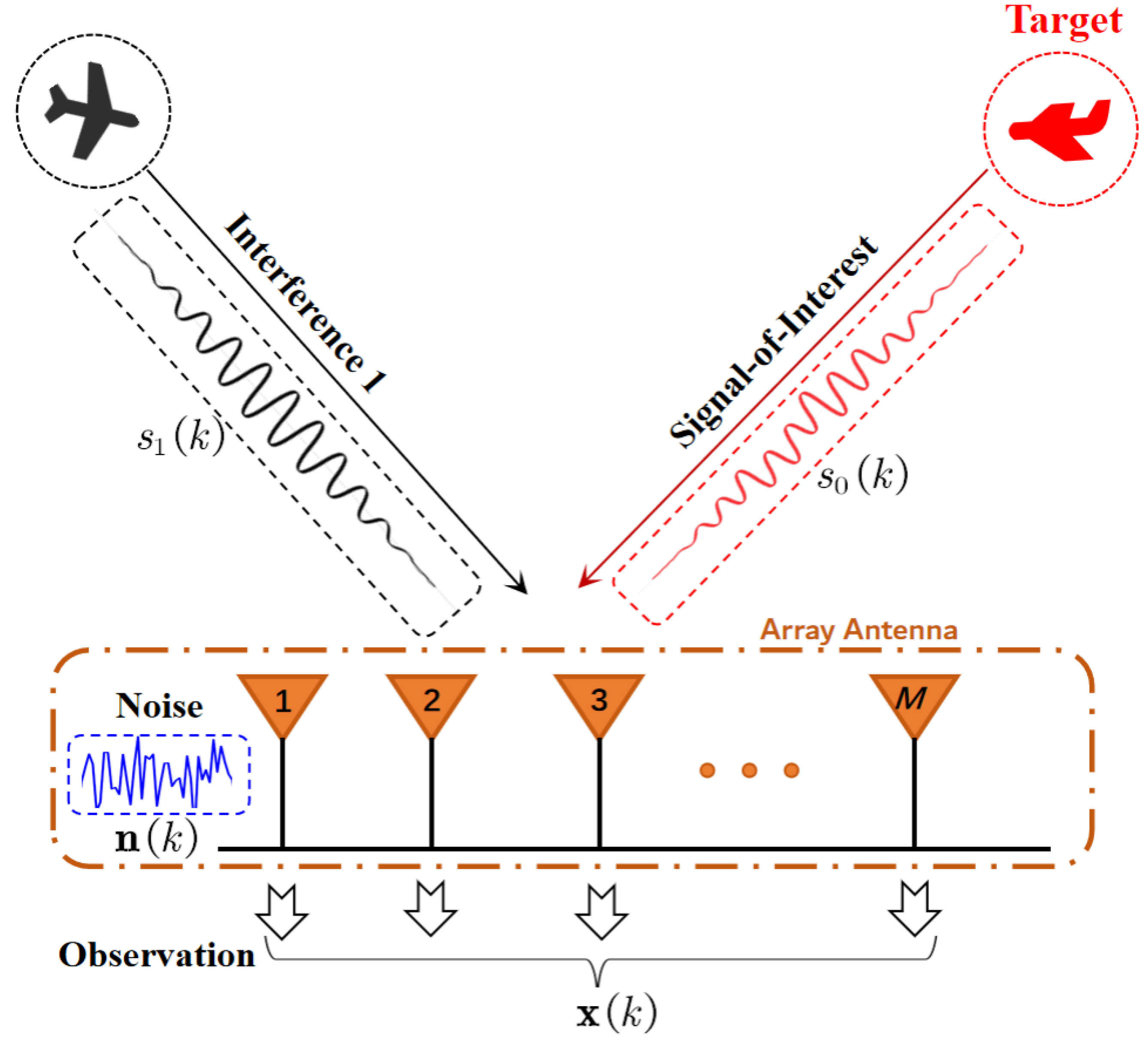
2. Signal Model and Background

Consider a linear array consisting of M isotropic sensors that receive narrowband signals from the far field. As depicted in Figure 1, the array observation data at time $k$ can be modeled as follows [32]:

$$x\left(k\right)=a_0{s}_0\left(k\right)+{\displaystyle \sum _{i=1}^{Q-1}{a}_i{s}_i\left(k\right)}+n\left(k\right)$$

(1)

where $a_0$ and $a_i$ denote the actual SVs of the SOI and ith interference, respectively; $s_0\left(k\right)$ and $s_i\left(k\right)$ denote the corresponding signal waveforms; $n\left(k\right)$ denotes the additive white Gaussian noise vector with covariance ${\sigma }_n^{2}I$. In this study, the sources and noise are assumed to be statistically uncorrelated with each other.

The output of a narrowband beamformer is given by:

$$y(k)=w^{H}x(k)$$

(2)

where $w$ represents the weight vector of the beamformer. It can be designed by maximizing the output SINR:

$$\mathrm{SIN}\mathrm{R}=\frac{{\sigma }_0^2{\left|w^H{a}_0\right|}^2}{w^H{R}_{\mathrm{i}+\mathrm{n}}w}$$

(3)

where ${\sigma }_0^2$ denotes the power of the SOI and $R_{\mathrm{i}+\mathrm{n}}$ is the theoretical INCM. The maximization of (3) can be solved by the following quadratic optimization problem:

$$\underset{w}{\min }{w}^H{R}_{\mathrm{i}+\mathrm{n}}w\hspace{1em}\mathrm{s}.\mathrm{t}.w^H{a}_0=1$$

(4)

which is the well-known MVDR beamformer. In practice, $R_{\mathrm{i}+\mathrm{n}}$ is rarely available. The following SCM $\widehat{R}$ is typically used:

$$\widehat{R}=\frac{1}{K}{\displaystyle \sum _{k=1}^{K}x(k)x^H(k)}=\frac{1}{K}X{X}^H$$

(5)

where $K$ denotes the number of snapshots and $X={\left\{x\left(k\right)\right\}}_{k=1}^K$ denotes the array snapshots. In addition, the exact SOI SV $a_0$ is replaced by the presumed SOI $\overline{a}$ in (4). In this case, the beamformer weight vector, which is referred to as the sample matrix inversion (SMI), is given by:

$$w_{\mathrm{SMI}}=\alpha {\widehat{R}}^{-1}\overline{a}$$

(6)

where the normalization constant $\alpha =1/\left({\overline{a}}^H{R}^{-1}\overline{a}\right)$ is immaterial and will therefore be omitted. Since the signal component exists in the SCM, the convergence rate of the SMI beamformer is known to be quite slow ($K\gg M$ is required [44]). Moreover, the SMI-based MVDR beamformer is sensitive to the mismatch between the presumed and actual SOI SVs.

3. Review of the Steering Vector Upgrade Methods

3.1. General Steering Vector Estimation Framework

To improve the robust performance of the above SMI-based MVDR beamformer, a famous uncertainty-set-based beamformer (often called the “robust Capon beamformer”) was proposed, which could obtain an estimate of the SOI SV by solving the following problem:

$$\begin{array}{l}\underset{a}{\min }{a}^H{\widehat{R}}^{-1}a\\ \mathrm{s}.\mathrm{t}.{\Vert a-\overline{a}\Vert }^2⩽\epsilon \end{array}$$

(7)

where $\Vert \cdot \Vert$ denotes the Euclidean vector norm, and the parameter $\epsilon$ stands for the uncertain set bound. The above optimization problem can be understood to maximize the output power for SVs in its defined uncertainty set. Since parameter $\epsilon$ is critical for beamforming performance but difficult to determine, some modifications have been proposed to renew the constraints; for example, some modifications are based on the outage probability [39], and others are based on the angular sector in which the SOI is located [40,41]. Moreover, an additional norm constraint ${\Vert a\Vert }^2=M$ can be imposed on the optimization problem to provide a better estimate.

In [43,45], the design of a general SVE framework was summarized as follows:

(i)

Maximize the output power (equivalently, by minimizing its reciprocal);

(ii)

Prevent the estimate of the SOI SV from converging to the interference SVs or their combinations;

(iii)

Add a norm constraint when appropriate to force the estimate to have the same norm as $\overline{a}$.

3.2. Conventional ESP Methods

As mentioned before, SOI SVs can be estimated using the optimization problem. Another path to obtain an enhanced SOI SV is by utilizing the ESP.

Let us write the eigen-decomposition of the SCM as:

$$\widehat{R}=U\Lambda U^H={\displaystyle \sum _{i=1}^M{r}_i{u}_i{u}_i^H}$$

(8)

where the unitary matrix $U=\left[u_1,\dots ,u_M\right]$ contains all normalized eigenvectors of $\widehat{R}$, and the diagonal elements of $\Lambda$ and $r_1>r_2>\dots >r_M$ are the corresponding eigenvalues. Here, the eigenvector matrix $U$ can be partitioned as $U=\left[U_{\left[Q\right]},{\overline{U}}_{\left[Q\right]}\right]$, where $U_{\left[Q\right]}=U\left(:,1:Q\right)$ consists of $Q$ dominant eigenvectors, and $U_{\left[Q\right]}$ spans the signal subspace (or SOI-plus-interference subspace); ${\overline{U}}_{\left[Q\right]}=U\left(:,Q+1:M\right)$ consists of the remaining subdominant eigenvectors, and ${\overline{U}}_{\left[Q\right]}$ spans the noise subspace or the orthogonal complement subspace of the signal subspace. As before, $Q$ stands for the number of incident signals.

An estimate of the SOI SV is obtained by projecting the presumed SOI SV onto the signal subspace:

$${\widehat{a}}_{\mathrm{p}1}=U_{\left[Q\right]}{U}_{\left[Q\right]}^H\overline{a}$$

(9)

Then, substituting ${\widehat{a}}_{\mathrm{p}1}$ into $\overline{a}$ in (6) yields the TESP beamformer [29]:

$$w_{\mathrm{TESP}}={\widehat{R}}^{-1}{\widehat{a}}_{\mathrm{p}1}={\widehat{R}}^{-1}{U}_{\left[Q\right]}{U}_{\left[Q\right]}^H\overline{a}$$

(10)

For the TESP, the projection subspace is spanned by $U_{\left[Q\right]}$, which is identified by the source number $Q$. Hence, the performance excessively relies on the adopted criteria of source enumeration. Furthermore, for low SNRs, a signal subspace swap may occur, resulting in the signal subspace being corrupted by the noise component.

Given the shortcomings of TESP, a robust adaptive beamformer named the MESP has been created [32], which reselects the projection subspace. As the mismatch between $\overline{a}$ and $a_0$ is not excessively large, the MESP points out that the eigenvectors corresponding to the large projections of $\overline{a}$ onto the eigenvector can be used to construct the projection subspace. Here, the values of the projections are given by:

$$p\left(i\right)={\left|u_i^H\overline{a}\right|}^2,i=1,\dots ,M$$

(11)

$p\left(i\right)$ can be arranged in descending order as follows, $p\left(k_1\right)⩾p\left(k_2\right)⩾\cdots ⩾p\left(k_M\right)$, where $k_i\in \mathbb{N},1⩽k_i⩽M$. Accordingly, the eigenvector matrix is reordered to obtain $\breve{U}=\left[u_{k_1},\dots ,u_{k_M}\right]$, and the eigenvalue matrix is changed to $\breve{\Lambda }$, of which the diagonal elements are reordered to be $r_{k_1},\dots ,r_{k_M}$.

The dimension of eigenvectors with large projection $T$ can be determined by:

$$\min \left(\frac{p\left(k_1\right)+p\left(k_2\right)+\cdots +p\left(k_T\right)}{M}\right)>\tau$$

(12)

where $\tau$ is a user-defined parameter and $0<\tau <1$. Then, the projection subspace can be spanned by a new structured matrix ${\breve{U}}_{\left[T\right]}=\left[u_{k_1},\dots ,u_{k_T}\right]$. Subsequently, the adaptive weight vector can be calculated as follows:

$$w_{\mathrm{MESP}}={\widehat{R}}^{-1}{\breve{U}}_{\left[T\right]}{\breve{U}}_{\left[T\right]}^H\overline{a}$$

(13)

For the MESP, the projection subspace is spanned by ${\breve{U}}_{\left[T\right]}$, which is structured by the eigenvectors corresponding to large projections of $\overline{a}$ onto the eigenvector $u_i$. This method needs a user-defined parameter $\tau$, that is, the threshold, to identify the “large projection”. However, there is no theoretical basis to support parameter selection.

In summary, regarding the determination of the projection subspace, the procedure of conventional ESP methods can be divided into two steps. First, the eigenvectors of the SCM are arranged in a certain order. The usage model of the arranged eigenvector matrix in the TESP is referred to as the eigenvalue ranking model, whereas the model in the MESP is referred to as the projection ranking model. Then, the arranged eigenvector matrix is partitioned into two, and the first part is taken as the spanning set, where the column dimension is selected by a criterion. The important indices of the two ESP methods are summarized in

Table 1. Summary of the two conventional ESP methods.

ESP-Beamformer	The Ranking Model of the Arranged Eigenvector Matrix	The Criterion of Dimension Selection for the Projection Subspace
TESP	Eigenvalue	The number of signal sources
MESP	Projection	The number of large projections exceeding a fixed threshold

.

In the next section, the eigenvector matrix is assumed to be arranged in advance. The task of this study is to select the subspace dimension via a unified criterion through which the performance of the ESP methods can be improved.

4. Proposed ESP Method

In this section, we first introduce a novel criterion of dimension selection for the projection subspace; that is, we use the sequenced SVE to derive the sequence number. Afterward, based on the criterion, we provide specific implementations for the two existing ranking models. For the eigenvalue ranking model used in TESP, we set a method without the requirement of source number estimation; for the projection ranking model exploited in the parameter-dependent method, MESP, we devise a parameter-free method.

4.1. Design of Sequenced Steering Vector Estimation

Hereafter, the arranged eigenvector matrix is uniformly denoted as $E$, the corresponding eigenvalue matrix is uniformly denoted as $L$, and the $i\mathrm{th}$ arranged eigenpairs are denoted as $\left(l_i,e_i\right)$. Then, the matrix composed of the first $n$ columns of $E$ can be denoted as $E_{\left[n\right]}$, and the $n\times n$ diagonal matrix $L_{\left[n\right]}$ contains the first $n$ eigenvalues of $L$. Based on the basis matrix $E_{\left[n\right]}$ of rank $n$, the SOI SV can be estimated as:

$$a_{\left[n\right]}=\beta E_{\left[n\right]}{E}_{\left[n\right]}^H\overline{a}$$

(14)

where the scalar variable $\beta =\sqrt{M}/\Vert E_{\left[n\right]}{E}_{\left[n\right]}^H\overline{a}\Vert$ is introduced to make the estimated and presumed SV norms coincide. Then, the collection of all available sequenced SVs can be grouped into a set $\left\{a_{\left[n\right]}\right\}=\left\{a_{\left[1\right]},\dots ,a_{\left[M\right]}\right\}$. To select a suitable SV from the above sequence, we now employ the general steering vector estimation framework. First, the maximum output power principle (equivalently by minimizing its reciprocal) can be taken into account:

$$\underset{n=1,\dots ,M}{\min }{a}_{\left[n\right]}^H{\widehat{R}}^{-1}{a}_{\left[n\right]}$$

(15)

In addition, to prevent the estimate from converging to the interference SVs or their combinations, we now introduce the correlation coefficient of two vectors, $s_1$ and $s_2$, which is generally defined as follows:

$$\rho (s_1,s_2)\triangleq \frac{\left|s_1^H{s}_2\right|}{\Vert s_1\Vert \Vert s_2\Vert }$$

(16)

It is assumed that the mismatch between the true SOI SV $a_0$ and the presumed SOI SV $\overline{a}$ is within an acceptable level. Generally, the interferences are considered incident from the sidelobe, and the correlation coefficients of $a_0$ and $\overline{a}$ should be significantly greater than that of $a_0$ and any interference SV. Accordingly, we can set a threshold for the correlation coefficient $\rho \left(a_{\left[n\right]},\overline{a}\right)$:

$$\rho \left(a_{\left[n\right]},\overline{a}\right)⩾\varsigma$$

(17)

where the parameter $\varsigma$ is the threshold and $0<\varsigma <1$. Note that (17) is equivalent to the uncertainty constraint in (7), for which the estimator is renewed from the estimator $a$ to ${a_{\left[n\right]}|}_{n=1}^M$(see Appendix A for proof). Combining (14), (15) and (17), the sequenced SVE process can be designed as follows:

$$\begin{array}{ll}\underset{n=1,\dots ,M}{\min }& a_{\left[n\right]}^H{\widehat{R}}^{-1}{a}_{\left[n\right]}\\ \mathrm{s}.\mathrm{t}.& \rho \left(a_{\left[n\right]},\overline{a}\right)⩾\varsigma \\ & a_{\left[n\right]}=\frac{\sqrt{M}{E}_{\left[n\right]}{E}_{\left[n\right]}^H\overline{a}}{\Vert E_{\left[n\right]}{E}_{\left[n\right]}^H\overline{a}\Vert }\end{array}$$

(18)

In the above problem, by substituting the inequality constraint and the objective function with the equality constraint and removing the immaterial scale value $M$ in the objective function, (18) can be reformulated as follows:

$$\begin{array}{l}\underset{n=1,\dots ,M}{\min }\frac{{\overline{a}}^H{E}_{\left[n\right]}{L}_{\left[n\right]}^{-1}{E}_{\left[n\right]}^H\overline{a}}{{\overline{a}}^H{E}_{\left[n\right]}^H{E}_{\left[n\right]}\overline{a}}\\ \mathrm{s}.\mathrm{t}.\frac{\Vert E_{\left[n\right]}{E}_{\left[n\right]}^H\overline{a}\Vert }{\sqrt{M}}⩾\varsigma \end{array}$$

(19)

Once the estimated basis matrix $E_{\left[\widehat{n}\right]}$ with the sequence number $\widehat{n}$ has been derived from (19), the projected SV can be obtained using the following:

$${\widehat{a}}_{\mathrm{new}}=E_{\left[\widehat{n}\right]}{E}_{\left[\widehat{n}\right]}^H\overline{a}$$

(20)

Note that the scalar variable $\beta$ in (14) has been omitted because it does not affect the output SINR. From the above discussion, the criterion for SVE can be used to invert the dimension of the projection subspace for the ESP. The estimated dimension $\widehat{n}$ can be directly obtained using (19) by adopting the enumeration method. However, the complexity is high. Another drawback is that it requires a user-defined parameter $\varsigma$. In view of this, we subsequently implemented (19) according to the concrete ranking models of $E$.

4.2. Selection of Subspace Dimension for Eigenvalue Ranking Model

In this subsection, we consider the eigenvector matrix arranged in the default ranking order according to the eigenvalue, which has been adopted by the TESP. In such cases, $E=U$ and $L=\Lambda$.

From Appendix B, it can be observed that the objective function in (19) increases monotonically with the sequence number $n$ in such cases. This implies that the optimal solution occurs in the smallest sequence number satisfying the constraint, i.e., the estimation problem (19) can be simplified as follows:

$$\underset{n=1,\dots ,M}{\min }n\hspace{1em}\mathrm{s}.\mathrm{t}.\frac{\Vert E_{\left[n\right]}{E}_{\left[n\right]}^H\overline{a}\Vert }{\sqrt{M}}⩾\varsigma$$

(21)

Here, the determination of the threshold $\varsigma$ is discussed. Recall that the inequality constraint in (21) is derived from $\rho \left(a_{\left[n\right]},\overline{a}\right)⩾\varsigma$, which is imposed to prevent the estimate of the projected SV from converging on the interference SVs or their combinations. Generally, the incident directions of interferences and the SOI differ. With a prior direction-of-arrival (DOA) of the SOI, an angular sector in which only the SOI is located can be built: $\Theta =\left[{\overline{\theta }}_0-\Delta \theta , {\overline{\theta }}_0+\Delta \theta \right]$, where ${\overline{\theta }}_0$ denotes the presumed DOA of the SOI, and $\Delta \theta$ is half the width of the angular sector. Based on the angular sector $\Theta$, the threshold can be chosen as:

$$\widehat{\varsigma }=\min \left(\rho \left(a_{{\mathrm{b}}^{-}},\overline{a}\right),\rho \left(a_{{\mathrm{b}}^{+}},\overline{a}\right)\right)$$

(22)

where $a_{{\mathrm{b}}^{-}}=d\left({\overline{\theta }}_0-\Delta \theta \right)$, and $a_{{\mathrm{b}}^{+}}=d\left({\overline{\theta }}_0+\Delta \theta \right)$ ($d\left(\theta \right)$ denotes the SV corresponding to the direction $\theta$ that has the structure defined by the antenna array geometry; for instance, $d\left({\overline{\theta }}_0\right)=\overline{a}$). By updating the constraint to $\rho \left(a_{\left[n\right]},\overline{a}\right)⩾\widehat{\varsigma }$, the estimate $a_{\left[n\right]}$ can be approximately restricted in the SV set associated with $\Theta$, of which the interferences lie outside. Although the presumed knowledge of the antenna array geometry is used to calculate $\widehat{\varsigma }$, this constraint is still sufficient when calibration errors exist, as demonstrated in the simulation.

In summary, the minimum $n$ ($n=1,\dots ,M$) satisfying the following expression can be obtained as the estimate of the subspace dimension for the eigenvalue ranking model.

$${\displaystyle \sum }_{i=1}^n{\left|e_i^H\overline{a}\right|}^2⩾M\cdot {\widehat{\varsigma }}^2$$

(23)

4.3. Selection of Subspace Dimension for Projection Ranking Model

Here, we focus on the dimension selection for the projection ranking model of the arranged eigenvector matrix, which is exploited in the MESP. In such cases,$E=\breve{U}$ and $L=\breve{\Lambda }$.

For any $n$, $\Vert E_{\left[n\right]}{E}_{\left[n\right]}^H{\overline{a}\Vert }^2⩾\Vert E_{\left[1\right]}{E}_{\left[1\right]}^H{\overline{a}\Vert }^2$; thus, it is easy to deduce the following:

$$\rho \left(a_{\left[n\right]},\overline{a}\right)⩾\rho \left(a_{\left[1\right]},\overline{a}\right)=\rho \left(e_{\left[1\right]},\overline{a}\right)$$

(24)

For the projection ranking model, $e_{\left[1\right]}$ is the single eigenvector corresponding to the largest projection onto $\overline{a}$; in other words, $\rho \left(e_{\left[1\right]},\overline{a}\right)=\max \left(\rho \left(e_{\left[\begin{array}{c}i\end{array}\right]},\overline{a}\right)\right),i=1,\dots ,M$. This implies that this orthogonal basis is bound to contain adequate SOI components. In such cases, (24) can at least prevent the estimate $a_{\left[n\right]}$ from approaching any interference SVs or their combinations.

Based on the above property, $\rho \left(e_{\left[1\right]},\overline{a}\right)$ can be understood as an appropriate threshold $\widehat{\varsigma }$ that has been set internally for the constraint when the projection ranking model is applied. Therefore, the inequality constraint in the optimization problem (19) can be eliminated. As a result, (19) can be reduced to the following nonparametric problem:

$$\underset{n=1,\dots ,M}{\min }\frac{{\overline{a}}^H{E}_{\left[n\right]}{L}_{\left[n\right]}^{-1}{E}_{\left[n\right]}^H\overline{a}}{{\overline{a}}^H{E}_{\left[n\right]}^H{E}_{\left[n\right]}\overline{a}}$$

(25)

Consequently, the estimate of the subspace dimension for the projection ranking model can be obtained using the following:

$$\widehat{n}=\arg \underset{n=1,\dots ,M}{\min }\frac{{{\displaystyle \sum }}_{i=1}^n\frac{1}{l_i}{\left|e_i^H\overline{a}\right|}^2}{{{\displaystyle \sum }}_{i=1}^n{\left|e_i^H\overline{a}\right|}^2}$$

(26)

Thus far, the proposed projection-based RAB methods can be delineated into the following steps:

Step 1.

Perform eigen-decomposition for the SCM $\widehat{R}$ and arrange the eigenvector matrix in a certain sorted order.

Step 2.

Estimate the projection subspace. Specifically,

(i)

If the eigenvalue ranking model is selected, i.e., $E=U$, the subspace dimension is estimated using (23).

(ii)

If the projection ranking model is selected, i.e., $E=\breve{U}$, the subspace dimension is estimated using (26).

Step 3.

Obtain the projected SV in (20) and calculate the beamformer weight vector as

$$w_{\mathrm{new}}={\widehat{R}}^{-1}{\widehat{a}}_{\mathrm{new}}$$

(27)

In the above steps, if (i) is taken in Step 2, we refer to the devised method as the proposed-EM. If (ii) is taken in Step 2, we refer to it as the proposed-PM. Suppose ${\widehat{n}}_{\mathrm{E}}$ and ${\widehat{n}}_{\mathrm{P}}$ denote the estimate of the subspace dimension for the proposed-EM and proposed-PM, respectively (${\widehat{n}}_{\mathrm{E}},{\widehat{n}}_{\mathrm{P}}\le M$). In the two proposed methods, the eigen-decomposition of the matrix $\widehat{R}$ in Step 1 costs the computational complexity of $\mathrm{O}\left(M^3\right)$. For the arrangement of the eigenvector matrix, the proposed-PM requires additional computations coming from (11) with the complexity of $\mathrm{O}\left(M^2\right)$. In Step 2, estimating the subspace dimension costs the computational complexity of $\mathrm{O}\left({\widehat{n}}_{\mathrm{E}}M\right)$ for the proposed-EM, and $\mathrm{O}\left(M^2\right)$ for the proposed-PM. In Step 3, obtaining the projected SV has the complexity of $\mathrm{O}\left({\widehat{n}}_{\mathrm{E}}M\right)$ for the proposed-EM, and $\mathrm{O}\left({\widehat{n}}_{\mathrm{p}}M\right)$ for the proposed-PM, and computing the weight vector in (27) has the complexity of $\mathrm{O}\left(M^3\right)$. Therefore, the overall complexities of the two proposed methods are both at the level of $\mathrm{O}\left(M^3\right),$ and are comparable to those of the TESP and MESP. For the INCM in [17], its computational complexity is dominated by the reconstruction of the covariance matrix and the solution of the QCQP problem. Therefore, the multiplication required by [17] is $\mathrm{O}\left(S{M}^2+M^{3.5}\right)$, where $S$ denotes the number of sampling points in the angular sector $\overline{\Theta }$ and $S\gg M$. Obviously, the proposed methods are more efficient than the INCM [17].

5. Simulation Result

Let us consider a uniform linear array of M = 10 identical isotropic sensors with an inter-element spacing of a half wavelength. The additive noise is spatially white Gaussian with unit variance. The SOI is nominally located at ${\theta }_0=10°$, and two interferences are incidents on the array from ${\theta }_1=-20°$ and ${\theta }_2=50°$. The input interference-to-noise ratios (INRs) of the two interferences are set to INR₁ = 30 dB and INR₂ = 25 dB. All the sources mentioned above are assumed to be narrowband and uncorrelated with each other.

In the following experiments, the imperfect array calibration model may be involved in some examples. Assume that the array perturbations contain magnitude and phase errors, along with sensor location errors. Specifically, the sensor gain errors are modeled as independent and identically distributed zero-mean Gaussian random variables with a standard derivation of 0.05. The sensor phase errors are assumed to be independent and uniformly distributed in $\left[-5°,5°\right]$. The sensor position error is uniformly drawn from [−0.05, 0.05] and measured in wavelengths.

In the proposed-EM, the DOA uncertainty set is chosen to be $\Theta =\left[{\theta }_0-5°, {\theta }_0+5°\right]$, except for where it is explicitly discussed in Example 1 and the simulation in Example 4.

The proposed methods are compared with the two conventional ESP-based methods and several baseline RAB methods. These beamformers are as follows:

(i)

ESP-based method 1: TESP [29], the dimension of the projection subspace is set to be the right number of the sources, ideally. That is, fixed to three under the simulation condition.

(ii)

ESP-based method 2: MESP [32], the user-defined parameter is chosen as $\tau =0.8$; this parameter is widely chosen and optimal for the simulation scenarios.

(iii)

Baseline method of DL type: Automatic DL (ADL) [10], a well-known DL-based RAB method, where the diagonal level can be calculated automatically without parameters.

(iv)

Baseline method of SVE type: RCB [37], a representative SVE-based RAB method. The uncertain set bound is set to $\epsilon =3,$ as in [37].

(v)

Baseline method of INCM type: INCM-based method proposed in [17]—the theoretical basis of such a type. The interference region is fixed at $\left[-90°,{\theta }_0-5°\right]{{\displaystyle \cup }}^{\hspace{1em}}\left[{\theta }_0+5°,90°\right]$; that is, the width of the SOI angular sector is $10°$, which is the same as that in [17].

The number of snapshots is set to $K=200$ unless stated otherwise. The optimal output SINR is plotted for benchmark, which is given by:

$${\mathrm{SIN}\mathrm{R}}_{\mathrm{opt}}={\sigma }_0^2{a}_0^H{R}_{\mathrm{i}+\mathrm{n}}^{-1}{a}_0$$

(28)

Two hundred Monte Carlo runs are performed for each simulation example. In the simulation results, the ESP-based RAB methods are indicated by solid lines, and the other RAB methods are indicated by dotted lines.

5.1. Example 1: Output SINR of Proposed-EM versus the Choice of $\Delta \theta$

In the first example, the effect of $\Delta \theta$ on the array output performance of the proposed-EM is discussed. As mentioned before, $\Delta \theta$ was the half-width of the angular sector $\Theta$ where the SOI was expected to be located. Three integer angles for $\Delta \theta$ were taken as prior information, all of which exceeded or were equal to the actual DOA error $\Delta {\theta }_0$. In this example, the SMI, TESP, and MESP were used for comparison. The following three cases were considered in this example:

(i)

The ideal condition, i.e., without any SV mismatch.

(ii)

SV mismatch due to fixed DOA mismatch, with the SOI nominally located at 13°; thus, the DOA error $\Delta {\theta }_0$ was fixed at 3°.

(iii)

SV mismatch due to fixed DOA mismatch and array perturbations, where the DOA error was the same as that in (ii), and the array perturbations were as indicated above.

Figure 2, Figure 3 and Figure 4 show the performance for different choices of $\Delta \theta$ versus the input SNR in the three cases. First, the condition of $\mathrm{SNR}\le -10\mathrm{dB}$ is discussed. From these figures, it can be found that a smaller $\Delta \theta$ leads to a better output SINR performance when $\mathrm{SNR}\le -10\mathrm{dB}$. However, the performance difference between the largest $\Delta \theta$ ($\Delta \theta =5°$) and the smallest $\Delta \theta$ ($\Delta \theta =3°$) was insignificant; there was an approximately 1.4 dB gap in the worst case at the point where the SNR took −30 dB in Figure 2. Moreover, whatever the value of $\Delta \theta$, the performance of the proposed-EM was significantly better than that of the TESP but was comparable to that of the MESP and SMI under such a low SNR condition.

Second, the condition of $\mathrm{SNR}>-10\mathrm{dB}$ is discussed. From Figure 2 and Figure 3, it can be seen that if the array calibration model was perfect, the best choice was $\Delta \theta =3°$, i.e., the value closest to the actual DOA error $\Delta {\theta }_0$. When $\Delta \theta$ took a coarse value satisfying $\Delta \theta >\Delta {\theta }_0$ (such as $4°$ or $5°$), the output SINR decreased as the SNR approached the jamming-to-noise ratio (JNR). The worst case appeared at the point that SNR took 30 dB in Figure 2, where the output SINR of choice, $\Delta \theta =5°$, was an approximately 3.2 dB gap from that of the best choice. Despite this, from the view of the entire SNR range, the proposed-EM with the choice $\Delta \theta >\Delta {\theta }_0$ could still obtain satisfactory performance compared with other ESP-based methods. If array perturbations existed, as shown in Figure 4, it was more appropriate to take a value slightly greater than $\Delta {\theta }_0$ for $\Delta \theta$ (such as $4°$ or $5°$), which would perform better at high SNRs. However, the choice $\Delta \theta =\Delta {\theta }_0$ was also reliable because, with this choice, the proposed-EM significantly outperformed the MESP and TESP, as depicted in Figure 4. It should be noted that the output SINR dropped at SNR around 30 dB regardless of the value of $\Delta \theta$. This was because the proposed-EM still belonged to the type of ESP scheme, which implied that it could not break through the inherent performance limitations of the ESP-based methods in the case when SNR was close to JNR.

Overall, the simulation results in Example 1 demonstrate that the performance of the proposed-EM was not very sensitive to the choice of $\Delta \theta$ if the DOA uncertainty set $\Theta$ was roughly obtained in advance. Moreover, as expected, even if array perturbations existed, this threshold setting was suitable for the determination of the projection subspace dimension.

In the following examples, the robustness of the two proposed methods is investigated through performance comparisons with the conventional ESP-based methods and some baseline RAB methods.

5.2. Example 2: Output SINR of Beamformers with Random DOA Mismatch

In the second example, the proposed methods are compared with other RAB methods in the scenario of SV caused by random DOA mismatch, where the DOA error is set to obey the uniform distribution of $\left[-5°, 5°\right]$.

Figure 5 evaluates the output SINR versus the input SNR of different methods. From this figure, the proposed-EM outperformed the proposed-PM at moderate SNRs (specifically, a 1.7 dB performance difference when $\mathrm{SNR}=20\mathrm{dB}$). Compared with the other ESP-based beamformers, the two proposed methods exhibited superior performance when $\mathrm{SNR}⩾-10\mathrm{dB}$. When the input SNR was less than $-$10 dB, the performance of the proposed methods was close to that of the MESP but significantly better than that of the TESP. For the RCB, due to the appropriate setting of the uncertain set bound, the curve could grow smoothly with the increase in SNR, but the output SINR was approximately 2.5 dB worse than that of the proposed methods when $\mathrm{SNR}⩾40\mathrm{dB}$. As no array perturbations existed in this example, the INCM reconstructed an ideal INCM; hence, its performance approached optimality. Figure 6 presents the output SINR versus the number of snapshots of different methods. It shows that, excluding the INCM, the two proposed methods and the TESP achieved the best performance among all tested beamformers, especially when the number of snapshots exceeded 50. As the number of snapshots exceeded 300, the output performance difference between the proposed methods and the INCM was within 1 dB, whereas the computational loads of the proposed methods were significantly lower than that of the INCM.

5.3. Example 3: Output SINR of Beamformers with Random DOA Mismatch and Array Perturbations

The third example examines a scenario with SV mismatch caused by random DOA mismatch and array perturbations. The setting for the random DOA error was the same as that in Example 2, and the model of array perturbations was as described previously.

Figure 7 plots the output SINR versus the input SNR of different methods, and Figure 8 displays the output SINR versus the number of snapshots of the different methods. Figure 7 shows that the performance of the ADL deteriorated more severely for high SNRs compared with Figure 5. This was because its parameter-free scheme was unsuitable for tackling the self-nulling problem in this scenario. In contrast, the proposed-PM, as another parameter-free RAB method, could provide a significantly improved robustness at high SNRs. Moreover, the proposed-PM significantly outperformed the MESP despite the same ranking model for the eigenvector matrix being used. This can be attributed to the reliable, parameter-free method in the proposed-PM. For the INCM, in terms of the existence of array perturbations, its performance degraded promptly owing to the poor anti-interference capability. Although the INCM outperformed the proposed methods when $\mathrm{SNR}⩾30 \mathrm{dB}$, it exhibited significant performance degradation in the weak SOI case. When $\mathrm{SNR}\le 10\mathrm{dB}$, in particular, the output SINR of the INCM was approximately $10\mathrm{dB}$ smaller than that of the proposed methods. In the entire SNR range, the proposed-EM achieved the best output SINR among the beamformers tested, and the proposed-PM also performed well, except for a small SINR decline when the input SNR was around $20\mathrm{dB}$. Figure 8 shows that the proposed methods and the TESP provided the best convergence performance among the beamformers tested within the entire range of snapshots. As the array was imperfectly calibrated, the INCM suffered the worst performance. In contrast, the proposed methods could still perform stably, as in the scenario with a perfect array manifold, as shown in Figure 6.

5.4. Example 4: Output SINR of Beamformers versus DOA Mismatches with Array Perturbations

In the fourth example, the output SINR versus the fixed DOA error is simulated when random sensor position perturbations exist. In practical scenarios, the DOA error may not be extremely large, and the angle deviation scope is set to be $\left[-6°,6°\right]$. In this example, the half-width of $\Theta$ was expanded to $6°$ for the proposed-EM so that the defined DOA uncertainty could tolerate all simulated DOA errors.

Figure 9 reveals that the proposed methods provided strong robustness against point errors. From Figure 9, the performance of the RCB and MESP was very close to our proposed methods when the DOA errors were less than 2$°$, but the performance of these methods degraded dramatically as the DOA errors exceeded $2°.$ Specifically, there was a 4.3 dB gap between the MESP and the proposed methods when the DOA errors were $3°$. The INCM, as in Example 3, performed poorly because of its high sensitivity to array perturbations. With the same ranking model for the arranged eigenvector matrix, the proposed-PM can offer greater resilience to large DOA errors than the MESP because of the effective nonparametric estimation approach. Furthermore, due to the appropriate threshold settings based on the accessible prior knowledge of $\Theta$, the proposed-EM can be robust in the entire range of simulated pointing errors. Through a comprehensive comparison, it can be observed that the two proposed methods and the TESP exhibited the best performance among the beamformers tested in this example.

6. Conclusions

In this study, a new insight into ESP-based RAB was presented. The proposed methods adopted sequenced SVE to determine the projection subspace. Based on this criterion, two implementations were developed for the existing ranking models of the arranged eigenvector matrix. Regarding the proposed-EM, a simple subspace dimension selection method was presented by exploiting prior information about the SOI angular sector; it can be executed without the requirement of source enumeration. Regarding the proposed-PM, after arranging the eigenvector matrix in a projection model, a parameter-free method was implemented for subspace dimension selection. The computational complexity of either proposed method is $\mathrm{O}\left(M^3\right)$, which is comparable to that of conventional ESP-based beamformers. It was demonstrated in the numerical examples that when the input SNR is as low as $-$30 dB, the proposed methods increase the output SINR by 5.4 and 6.1 dB over the TESP in the presence and absence of array perturbations, respectively. In the case of moderate SNRs, the proposed methods provide at least a 4.3 dB output SINR improvement over the MESP when the DOA errors exceed $3°$. Compared with the INCM, the proposed methods exhibit less sensitivity to array perturbations; specifically, the output SINR of the proposed methods is approximately 10 dB larger than that of the INCM at low SNRs in such a case. In addition, the proposed methods exhibit good convergence performance, where the output SINR is only 2 dB lower than the optimal value when the number of snapshots exceeds 300. The overall simulation results demonstrate the improvement of the conventional ESP-based RAB methods and their robustness against various SV mismatches.