Comparative Analysis of Machine Learning Techniques for Non-Intrusive Load Monitoring

Abstract

Non-intrusive load monitoring (NILM) has emerged as a pivotal technology in energy management applications by enabling precise monitoring of individual appliance energy consumption without the requirements of intrusive sensors or smart meters. In this technique, the load disaggregation for the individual device is accrued by the recognition of their current signals by employing machine learning (ML) methods. This research paper conducts a comprehensive comparative analysis of various ML techniques applied to NILM, aiming to identify the most effective methodologies for accurate load disaggregation. The study employs a diverse dataset comprising high-resolution electricity consumption data collected from an Estonian household. The ML algorithms, including deep neural networks based on long short-term memory networks (LSTM), extreme gradient boost (XgBoost), logistic regression (LR), and dynamic time warping with K-nearest neighbor (DTW-KNN) are implemented and evaluated for their performance in load disaggregation. Key evaluation metrics such as accuracy, precision, recall, and F1 score are utilized to assess the effectiveness of each technique in capturing the nuanced energy consumption patterns of diverse appliances. Results indicate that the XgBoost-based model demonstrates superior performance in accurately identifying and disaggregating individual loads from aggregated energy consumption data. Insights derived from this research contribute to the optimization of NILM techniques for real-world applications, facilitating enhanced energy efficiency and informed decision-making in smart grid environments.

1. Introduction

The rising demand for an increased proportion of renewable energy resources (RES) in the coming decades, driven by the cost-effectiveness and environmental benefits of cleaner energy production, is expected to follow an upward trajectory [1]. Although RES contributes positively to sustainability and environmental concerns, their intermittent nature poses challenges in the residential energy sector [2,3]. Therefore, it is crucial to strike a balance between demand and supply to effectively manage these energy resources. The inclusion of shiftable and non-essential loads in the residential sector, such as electric vehicles (EV) and battery energy storage systems (BESS), can play a pivotal role in optimizing energy management and enhancing system flexibility. The strategy involves scheduling these loads to coincide with the availability of RES-like photovoltaic (PV) energy. This approach not only reduces energy consumption costs and promotes sustainability and self-reliance but also augments the penetration of renewable energy [4]. Referred to as energy flexibility (EF), this adaptability is essential for transitioning towards eco-friendly and efficient energy grids. A noteworthy development in this context is the emergence of demand-side energy aggregators, which contribute to balancing demand and supply by minimizing peak loads during periods of high demand, thereby ensuring stability in power systems, and facilitating EF [5].

The EF is generally referred to as the customer’s capacity to adjust or modify behavior based on energy demand, production variations, weather conditions, and user or grid requirements [6,7]. Several devices in the household are known as shiftable loads such as EVs, washing machines, dishwashers, etc. These devices are not essential and could be used at a later time, therefore, referred to as shiftable/movable devices. Another prevalent definition focuses on the earliest start time and ending time of shiftable devices. Traditional EF characterization involved installing smart meters on residential devices and continuously monitoring data, which, although straightforward, could be costly and slow it also raised concerns about data privacy [8].

A new approach, non-intrusive load monitoring (NILM), has been proposed as an alternative. NILM observes the usage patterns of devices based on their current signals, eliminating the necessity for smart meters [9]. The total energy consumption of the user is given to the NILM model as an input and then the device usage times are extracted, this method is known as load disaggregation. This makes NILM an essential tool for demand-side management (DSM) and EF applications. Although the most precise method to measure device usage is through energy meters on individual devices, this approach is not the most practical [10]. The integration of data-driven technologies, such as machine learning (ML), into NILM has enhanced its efficiency. A detailed review of the NILM method is given in [11]. NILM solutions can be categorized into supervised and unsupervised learning [12]. In supervised learning, the model is trained using a dataset, followed by testing and verification. On the other hand, unsupervised learning involves the model extracting information from data and forming clusters without prior training sets [13]. While unsupervised learning is faster and more convenient, it lacks the accuracy of supervised learning [14]. Several ML-based methods, including K-nearest neighbor (kNN), neural networks, support vector machine (SVM), deep learning (DL), and event matching classification, have been proposed in supervised NILM. There are many studies that have also incorporated statistical methods such as particle swarm and Markov chain models. In

Table 1. Comparison of the current study with existing literature.

Study	Year	Place	Method Used for NILM	Dataset	Avg. Efficiency (%)
[15]	2019	China	Particle swarm	1 year	94.2
[16]	2023	Indonesia	Random Forests	1 year	99
[17]	2020	India	Markov Chain	31 days	94
[5]	2021	Estonia	Extreme Gradient Boost (XgBoost)	3 years	97.2
[18]	2022	Malaysia	K-NN, SVM, Ensemble	30 days	98.8
[19]	2020	Iran	SVM	1 week	98.2
[20]	2021	Indonesia	Convolutional Neural Networks (CNN)	1 month	98
[21]	2023	Italy	Random Forests	27 months	96.3
[22]	2024	Spain	Long Short-Term Memory Networks (LSTM)	7 months	98
[23]	2023	Greece	Recurrent Neural network (RNN)	10 days	97
[24]	2023	Canada	LSTM	2 days	98
[25]	2023	UAE	Current Waveform Features with Rule-Based Set Theory (CRuST)	1 month	96
This Study	2024	Estonia	DTW-KNN, Logistic Regression (LR), XgBoost, RNN-LSTM	1 year	98

, a comparison of previous studies with this study has been presented.

The NILM method has been used for anomaly detection at the appliance level by incorporating machine learning [26]. In another study [8], NILM is utilized for the event matching of devices. This study was based on the Pecan Street dataset, and it used a deep learning algorithm for this event matching. In [27], the NILM technique is used to identify the load patterns, and then later, these patterns are used to improve the accuracy of the load forecasting. A NILM-based solution has been proposed for energy management in microgrids [28]. Furthermore, the solution also provides input for the electricity market based on the load characterization by NILM. The results indicated that using this technique the energy costs and load curtailment can be reduced. In [29], a NILM-based algorithm has been proposed for the monitoring of loads in the power distribution network. This technique consists of a neural network and improves accuracy by 5%.

In most of the literature presented above, there are several methods used in NILM modeling. However, the accuracy of these NILM models is challenging as there are many device variations, different manufacturers with different power ratings and device operating modes. The inclusion of ML and DL methods improves this performance significantly but still, these methods require larger datasets of reference device signals which is problematic. Therefore, there is a gap in the research studies about the comparison of different ML and DL algorithms on the accuracy of the NILM technique. Moreover, the impact of the size of the dataset on the performance of NILM is also of interest. This paper tries to fill this gap by evaluating the performance of several ML and DL algorithms employed in NILM. These models are designed based on a real-life dataset measured in an Estonian household for the whole year. These are the main contributions of this work:

• Thorough comparative analysis of ML Techniques for NILM, revealing optimal methodologies for load disaggregation.
• Utilization of diverse dataset from an Estonian household for comprehensive evaluation of ML algorithms.
• Implementation and Evaluation of LSTM, XgBoost, LR, and DTW-KNN models, highlighting XgBoost’s superior performance.
• Insightful evaluation metrics application includes accuracy, precision, recall, and F1 score for nuanced assessment.
• Identification of XgBoost as the most effective model for load disaggregation, offering practical implications for enhancing energy efficiency.

The rest of the article is structured as follows: Section 2 provides detailed background information about NILM and the ML and DL methods used in this research. The case study of the Estonian household and the development of these NILM models are presented in Section 3. The results and discussion are given in Section 4. Finally, the conclusion and future works are summarized in Section 5.

2. Non-Intrusive Load Monitoring (NILM)

Non-Intrusive Load Monitoring (NILM) is a progressive approach for estimating individual appliance operating states and their energy consumption based on household total electrical load measured at a single point. It involves acquiring and disaggregating the overall electricity usage, offering a simple and cost-effective means of monitoring appliances’ operation and energy consumption formulated as:

$$P_{total}\left(t\right)={{\displaystyle \sum }}_{k=1}^K{p}_k\left(t\right)+e\left(t\right)$$

(1)

where

$P_{total}\left(t\right)$ is the power consumed by all appliances,

$p_k$(t)—power consumed by the kth appliance,

$e\left(t\right)$—error or difference between aggregate meter reading and the sum of actual power consumption.

The examination relies on the measurement of voltage and current waveforms taken at the electrical service entrance (ESE). These data serve as the basis for deducing the operational conditions and power consumption of each individual load. Load signatures, also known as load features, are derived from these waveforms, providing measurable parameters that reveal information about the nature and operating status of individual appliances. Appliances can be categorized into distinct types based on their load signatures, shaping the approach to disaggregation:

• Type-I appliances, such as toasters and boilers, exhibit a straightforward ON/OFF state.
• Type-II devices like washing machines and ovens operate with multiple (finite) number of operating states with recognizable patterns.
• Type-III devices, presented by dimmer lights, belong to continuously variable devices (CVD), presenting a challenge in disaggregation due to their constantly varying consumption.
• Type-IV, devices that are constantly in operation and have different energy consumption modes like smoke detectors and refrigerators.

Given the diversity outlined above, developing an accurate yet broadly applicable NILM system is a challenging task. Consequently, many algorithms are designed to focus on identifying only the most significant appliances. This strategic approach acknowledges the complexity of capturing the varied operational signatures across different appliance types while aiming to provide targeted and effective load disaggregation. 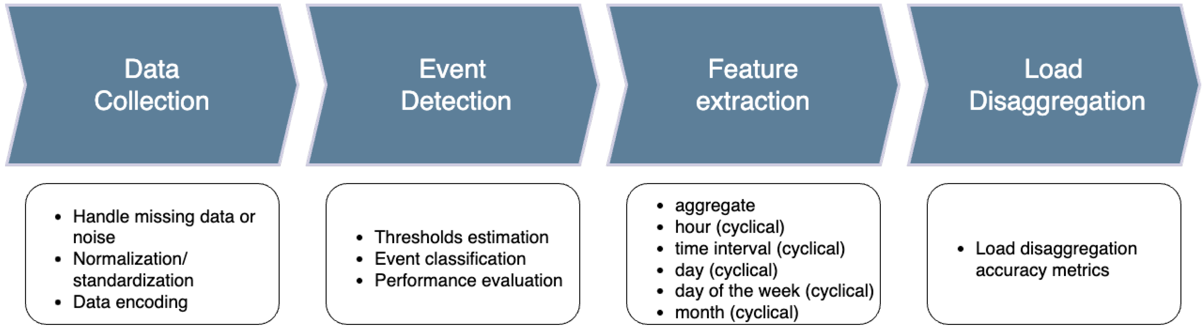The goal is to strike a balance between accuracy and generalization, ensuring that the NILM system can reliably identify and monitor key appliances without becoming overly intricate and challenging to implement [30,31]. A general NILM process can be presented in four phases and observed in Figure 1.

2.1. Data Collection

The initial step in any NILM algorithm involves data acquisition, typically obtained from smart meters. The crucial question in load disaggregation is determining the optimal data collection frequency for smart meters to ensure accurate appliance identification and power estimation. The trade-off between high and low data frequencies significantly impacts NILM algorithm effectiveness. High-resolution measurements, often exceeding 1 Hz, can extract transient features crucial for identifying appliances with similar power consumptions, particularly during state transitions. On the other hand, excessively small data frequencies limit feature extraction to steady-state characteristics, proving it insufficient for differentiating appliances with comparable power usage.

The sampling frequency, an essential factor in data pre-processing, varies based on the appliance signature of interest, with researchers recognizing the utility of both low-frequency and high-frequency signatures. High-frequency data, however, require high-end hardware, additional data storage, and have transmission problems, and thereby increasing costs. Recent NILM solutions strategically balance algorithmic efficiency and performance across a diverse range of appliances, often favoring low-frequency signals to achieve satisfactory results [32].

The algorithms differ significantly in their approach to handling data at the collection stage. The below-mentioned algorithms have the following differences: DTW-KNN excels in time series classification, accommodating speed variations but lacks explicit handling of missing data or noise. XgBoost robustly handles tabular data, automatically adapting to missing data and outliers, despite needing careful tuning and pre-processing. Logistic Regression, suitable for binary classification, demands meticulous pre-processing, especially for categorical data, and lacks inherent handling of missing values and noise. LSTM networks, an expert at processing sequential data, are robust to noise but may struggle with lengthy sequences, necessitating truncation or summarization and requiring numerical input. Based on the above mentioned each algorithm offers unique strengths, and optimal performance relies on meticulous data pre-processing and tuning tailored to the task and data characteristics.

2.2. Event Detection

Within the domain of NILM, event detection serves as a crucial task, focusing on detecting state transition actions generated by appliances. The event detection module identifies instances of state transitions in the aggregated power signal, characterizing actions like ON/OFF switches, changes in appliance speed and mode alternations. Challenges in event detection arise from high fluctuations, long transitions and near-simultaneity, and misidentification of events can lead to decreased accuracy and increased computational complexity in NILM methods. The event detection module employs various models, including expert heuristics, probabilistic models, and matched filter models, to identify events in the aggregate signal, with a subsequent focus on exploring different signatures for effective NILM research, including steady-state features extracted from low-frequency sampled data around the event detection window. Despite their ease of extraction, steady-state features face challenges of feature overlapping and susceptibility to power disturbances, highlighting the ongoing efforts to enhance NILM methodologies [30].

In the event detection phase, the process begins with threshold estimation, where a specific value is set or calculated dynamically to identify when an event, such as an appliance turning on or off, has occurred. This threshold is typically based on changes in power consumption and aims to minimize both false positives and negatives. Following the detection of events, they are classified into different categories, often corresponding to individual appliances. The performance of this event classification is then evaluated using various metrics such as precision, recall, and F1-score. These metrics assess the accuracy of the classification in terms of the proportion of correctly identified events, the proportion of actual events that were missed, and the balance between precision and recall, respectively.

2.3. Feature Extraction

Effective NILM methods necessitate distinctive features or signatures that capture the unique behaviors of appliances, facilitating the differentiation of various types of appliances. These features are derived from the distinctive power consumption patterns exhibited by individual appliances and are utilized to identify or recognize corresponding appliances from aggregated signals. Two main categories of features employed in NILM are transient features and steady-state features. Transient features, extracted from the transition process between two steady states, require high-frequency data acquisition by smart meters, typically exceeding 1 Hz. Event detection methods separate the transition process from overall measurements, posing a challenge to accurately capture the start and end of transitions. The steady-state features, on the other hand, encompass variables such as active power, reactive power, current, and voltage waveform, and can be extracted from conventional smart meter data without the need for high-frequency sampling. Although steady-state features are commonly used, determining the number of states remains challenging [30,33].

Feature extraction is a crucial step that involves processing the collected data to extract meaningful information. Features mentioned above (see Figure 1) can be used individually or in combination to improve the performance of the systems. For example, “aggregation” refers to the total energy consumption data collected from the main power line. It serves as the primary input for NILM systems. Date/time features can capture daily/weekly/monthly/annual patterns in energy usage. Time intervals can refer to the duration for which an appliance is used, as different appliances tend to be used for different lengths of time [31,32]. These features can be used individually or in combination to improve the performance of NILM systems. The choice of features often depends on the specific characteristics of the problem at hand, such as the number of appliances, the sampling rate of the data, and the availability of training data [33,34].

2.4. Load Disaggregation

The final stage in the process is load disaggregation, where the identified features and patterns are used to determine the individual energy consumption and operational states of specific appliances within a building. During the load disaggregation phase, machine learning or pattern recognition algorithms, previously trained on labeled datasets in the earlier stages, are applied to the real-time or historical aggregated energy data [35]. These algorithms use the learned patterns and features to attribute portions of the total energy consumption to specific appliances. The complexity of load disaggregation lies in the fact that multiple appliances may be operating simultaneously, and their energy signatures may overlap. Advanced machine learning models are often employed to handle these challenges and improve the accuracy of disaggregation. The choice of algorithm often depends on specific characteristics of the data and the complexity of the task, including the number and types of appliances, the intricacy of energy usage patterns, and the availability of labeled training data [36].

Recognizing the diverse nature of energy consumption patterns, a strategy involving multiple algorithms has been chosen. NILM studies have explored both supervised and unsupervised approaches. Supervised methods, utilized in our approach, require a labeled dataset with sub-metered appliances. However, this kind of dataset may not always be available. On the other hand, unsupervised methods can be applied without prior knowledge of the environment. Nevertheless, users are required to validate identified appliance patterns. As our data are labeled, we primarily use supervised methods in our approach. Dynamic Time Warping (DTW) is employed for its ability to measure similarity between sequences, providing flexibility in capturing dynamic variations in energy consumption. The K-NN algorithm leverages the proximity of data points to classify patterns, contributing a robust method for identifying similarities in energy signatures. XgBoost, a powerful ensemble learning technique, excels in handling complex relationships and boosting predictive performance [37]. Lastly, LSTM is chosen for its effectiveness in discerning patterns in high-dimensional spaces [38]. By integrating these algorithms, we aim to enhance the accuracy and versatility of our load disaggregation process, addressing the complexities inherent in energy consumption data.

3. Machine Learning Techniques

ML revolutionized NILM by providing transparency and precision in energy consumption analysis. ML algorithms excel at analyzing vast datasets and uncovering hidden patterns within the energy signal. They can learn from historical data to identify unique signatures of individual appliances, even when operating simultaneously. ML’s dynamic nature allows it to adapt continuously to evolving usage patterns and seasonal variations, ensuring sustained accuracy over time. Ultimately, ML transforms raw energy data into actionable insights, empowering users to optimize energy management.

3.1. Dynamic Time Warping with K-Nearest Neighbor (DTW-KNN)

DTW is a crucial algorithm for time series classification, where the objective is to train a model capable of accurately predicting the class of a time sequence within the labeled dataset [39]. The K-NN algorithm is commonly employed for this task, with a modification using the DWT metric instead of the classic Euclidian distance. DTW accommodates variations in length and speed between the compared time series, making it particularly effective for capturing patterns in energy consumption over time [40]. Despite its efficiency, the challenge lies in the time complexity of DTW, especially for large datasets with lengthy sequences [41]. However, understanding the nuances of DTW allows for necessary adjustments to enhance the algorithm’s speed, ensuring practical and efficient time series classification in the context of NILM.

For one-dimensional time series denoted as f(x(i)) and f(y(j)), where i and j represent time points in series, and x and y are vectors, characterized by their Euclidian distances [42]. The DTW algorithm involves creating a local cost matrix D storing pairwise distances between x and y. The algorithm seeks an optimal warping path under certain constraints using dynamic programming, determining the DTW distance as the minimum accumulated distance normalized by the length of the optimal warping path. This alignment process minimizes the “distance” between the two-time series is presented in Equation (2):

$$D_{i,j}=d\left(x_i,y_j\right)+\min \left\{\begin{array}{c}{D}_{i-1,j-1}\\ D_{i-1,j}\\ D_{i,j-1}\end{array}\right.\begin{array}{c}\left(\mathrm{match}\right)\\ \left(\mathrm{insertion}\right)\\ \left(\mathrm{deletion}\right)\end{array},$$

(2)

where $d\left(x_i,y_j\right)=\left|x_i-y_j\right|$.

The k-nearest neighbors (K-NN) nonparametric statistical algorithm relies on k training samples in proximity to the feature space as input. The classification of an object is based on the most frequently occurring class among the identified k nearest points. The parameter k denotes the number of nearest neighbors influencing the classification process, and the selection of an appropriate k is a nuanced yet crucial step for optimizing the model’s performance [43].

The integration of DTW and K-NN in a combined approach is motivated by the distinctive strengths of each method. This integration yields a more robust and accurate predictive model, specially tailored for applications in time series analysis. Essentially, the synergy between DTW and K-NN capitalizes on DTW’s efficacy in capturing temporal nuances and K-NN’s proficiency in pattern classification based on similarity. This combined approach facilitates a more comprehensive analysis of time series data, proving particularly beneficial when dealing with complex and dynamic patterns [43].

3.2. Extreme Gradient Boosting

XgBoost is a highly efficient machine learning algorithm known for its effectiveness in predictive modeling tasks. As a gradient-boosting algorithm in the ensemble learning family, XgBoost excels in capturing intricate patterns and relationships within energy consumption data [44]. Its strength lies in accurately identifying and distinguishing between energy signatures of diverse appliances, making it invaluable in scenarios with complex and evolving consumption behaviors [44,45]. Operating as a tree ensemble model with k trees XgBoost predicts outcomes for data samples $\left(x_i,y_i\right)$ through a defined expression [46]:

$$\widehat{y_i}=F_k\left(x_i\right)=F_{k-1}\left(x_i\right)+f_k\left(x_i\right),$$

(3)

where

$F_{k-1}\left(x_i\right)$ is the prediction result of previous $k-1$ trees,

$f_k\left(x_i\right)$—$k$-th decision tree.

The algorithm’s objective function involves a cost function, assessing the error between predicted and actual values.

$$F_{obj}={{\displaystyle \sum }}_{i=1}^{n}L\left(y_i,\widehat{y_i}\right)+{{\displaystyle \sum }}_{j=1}^k\Omega \left(f_j\right)$$

(4)

The regularization term incorporates the L1-norm, preventing overfitting by penalizing the number of leaf nodes, and the L2-norm, penalizing leaf node weights. Each iteration introduces a new tree, and the objective function is approximated using first and second-order gradients.

3.3. Logistic Regression

Logistic regression plays a pivotal role in load disaggregation within NILM systems for binary classification tasks, determining the ON/OFF states [47]. In this context, logistic regression models are trained using labeled data where the state of each appliance is known. Features extracted from the aggregated power signal, such as voltage, current, and frequency, serve as input variables for the logistic regression model. The model learns the relationship between these features and the probability of an appliance being in the on or off state [48].

During inference, the trained logistic regression model is applied to real-time aggregated power data to predict the probability of each appliance being ON or OFF. By setting a threshold probability, appliances are classified as either ON or OFF, providing valuable insights into individual appliance usage patterns. The performance of the regression-based load disaggregation model is then evaluated using metrics such as accuracy and precision and recall, with iterative optimization techniques like feature selection and hyperparameter tuning applied to enhance model efficacy.

3.4. Long Short-Term Memory Networks (LSTM)

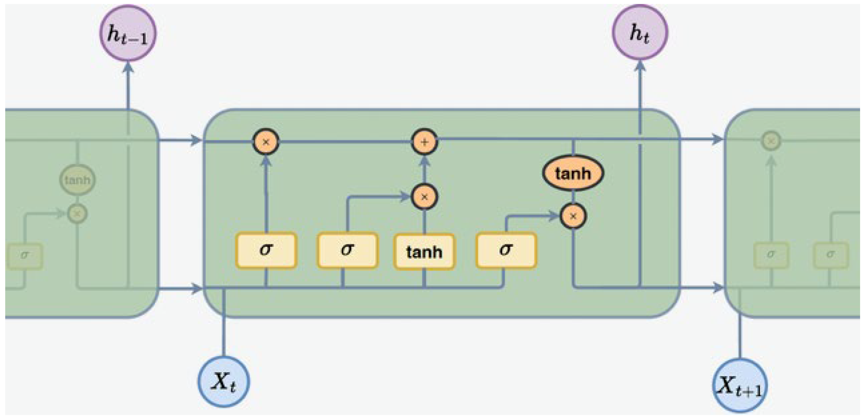
The LSTM algorithm has become one of the essential tools in NILM due to its ability to overcome the limitations of traditional Recurrent Neural Networks (RNNs), especially in handling long-term dependencies and gradient vanishing issues [49]. LSTMs are particularly favored for NILM tasks because they excel at capturing the inherent long-term dependencies present in time series data. Equipped with forget, input, and output gates, the LSTM architecture provides precise control over information flow within each memory block, allowing for the retention of relevant information while discarding extraneous data.

The hidden layer of an LSTM network is a crucial component comprising gated units or cells, which work in tandem to generate both the cell’s output and internal state (see Figure 2). Consisting of four interconnected elements, including three logistic sigmoid gates and one hyperbolic tangent (tanh) layer, LSTMs exhibit a sophisticated mechanism for controlling information flow within the cell [50]. The forget gate, employing a sigmoid activation function, determines the relevance of information from the previous cell state, aiding in the removal of obsolete data. Subsequently, the input gate combines current input with the previous hidden state, filtering pertinent information and generating new candidate values for the cell state through a tanh layer. Finally, the output gate normalizes cell state values and produces the final output, emphasizing LSTMs’ capability to retain long-term dependencies and regulate information flow effectively [51].

It is essential not to overlook the need for additional signal processing when integrating neural networks (NNs) into applications. Circular timestamps provide a cyclic representation of time, which is beneficial for handling periodic data such as daily or seasonal patterns. They enable neural networks, especially LSTM models, to better capture recurring patterns in tasks like time series forecasting and energy consumption modeling [52]. When using circular timestamps with LSTMs, it is crucial to encode timestamps as angles on a unit circle and design networks to handle circular sequences effectively. This approach enhances LSTM models’ ability to accurately learn cyclic patterns across diverse domains, offering a compact yet powerful representation of time-related data [53].

3.5. Performance Indicators

Evaluating NILM systems requires careful consideration since a single metric cannot capture all its nuances. Although metrics like mean squared error (MSE) and false positive/negative rates offer insights into overall accuracy, the evaluation should extend to specific appliance identification metrics such as precision, recall, and F1-score [22]. These metrics provide a granular understanding of how well the system distinguishes between individual appliances, which is essential for practical implementation in real-world scenarios [10,43].

$$Precision=\frac{TP}{TP+FP},$$

(5)

$$Recall=\frac{TP}{TP+FN},$$

(6)

$$F1=2\frac{Precision\times Recall}{Precision+Recall}.$$

(7)

A confusion matrix is a fundamental technique in machine learning that serves as a concise summary of a classification algorithm’s performance. It provides a tabular layout of the correct and incorrect predictions made by the classifier, mapping these predictions to the original classes of the data. This matrix offers crucial insights that go beyond simple accuracy metrics, which is especially valuable when dealing with imbalanced datasets or multiple classes. In the matrix, columns denote predicted values, while rows represent actual values. This arrangement offers a clear visualization of the model’s accuracy and the patterns of its errors across all classes simultaneously. This structured grid aids in understanding the classifier’s performance by comparing the correct and incorrect predictions for each class.

The evaluation, however, does not end at core performance metrics. Computational efficiency, adaptivity, and data handling diversity must also be considered. Metrics such as execution time and memory usage shed light on the system’s computational demands, crucial for real-time applications and resource-constrained environments. Flexibility metrics gauge the system’s ability to adapt to new appliances and environmental changes, ensuring its relevance and applicability over time. Finally, scalability and robustness metrics assess how well the system performs across diverse datasets and under varying conditions, offering a comprehensive picture of its reliability and generalizability.

4. Case Study of an Estonian Household

4.1. Exploratory Data Analysis

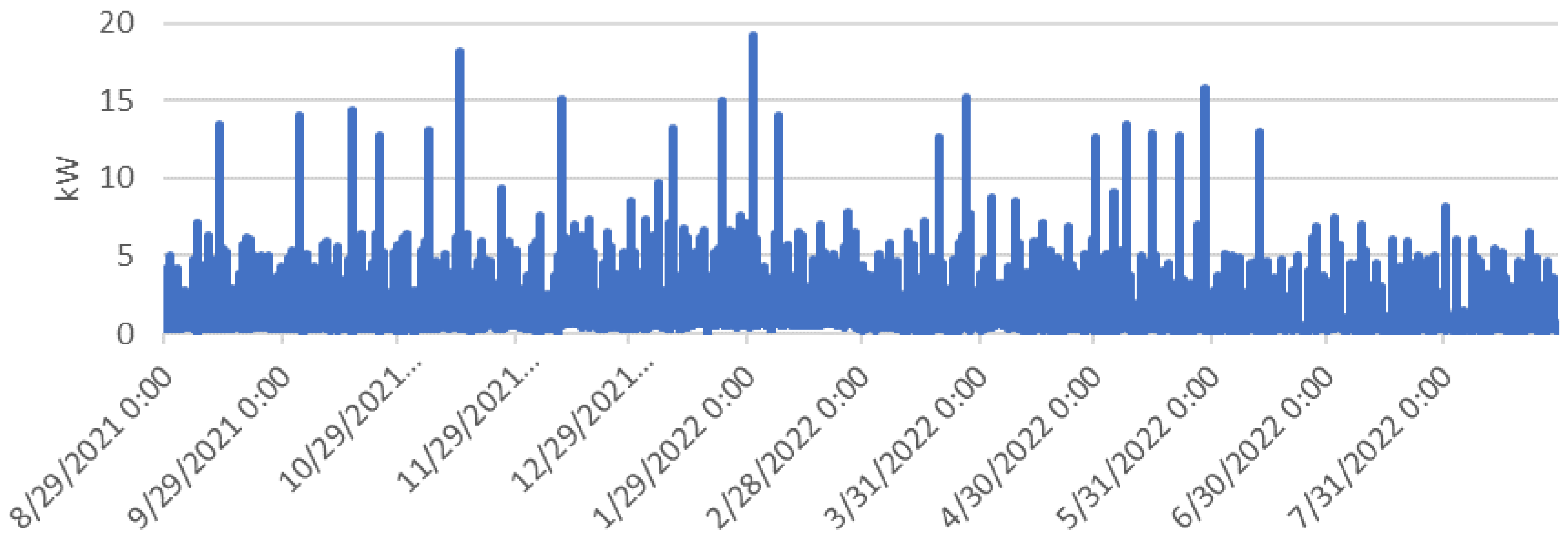
In this study, forecasting algorithms were developed using load data from a household in Estonia. The specific residence is situated in Tallinn city, comprising two levels, four rooms, and holding a “C” energy rating. With a total area of around 100 square meters, it was designed for two adults and one child. The data was measured using the Emporia Gen 2 3-PHASE device with 16 Sensors. Data collection spanned from August 2021 to August 2022, achieving an accuracy rate with an error margin below 5%. Measurements were taken at 15-min intervals. The analysis included various household appliances such as a dishwasher, vacuum cleaner, television, stereo, sauna, ventilation system, refrigerator, lighting fixtures, electric stove, and washing machine. Additionally, the house featured a heating system, water heater, and electric heating floor. The key DC power consumers in the residence comprised interior and exterior lights, multiple phone and laptop chargers, a TV and sound system, and a floor heater.

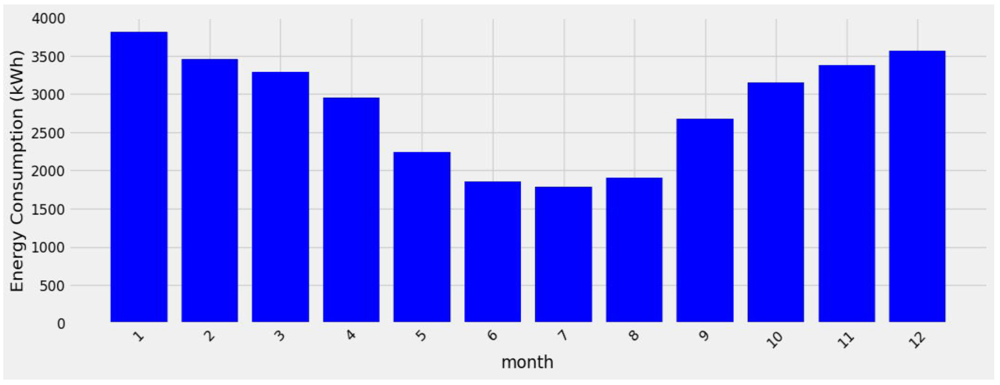
The data for the entire year is illustrated in Figure 3, showcasing separately measured AC and DC loads within the household. The combined average value loads hours around 3 kW. The peak recorded load, reaching approximately 19 kW, occurred in February during the winter months when heating demands were at their peak. In Estonia, winter spans from November to March, typically witnessing higher energy consumption. Conversely, during the summer months between May and August, energy consumption drops significantly as heating demands diminish. The monthly energy consumption throughout the year is shown in Figure 4.

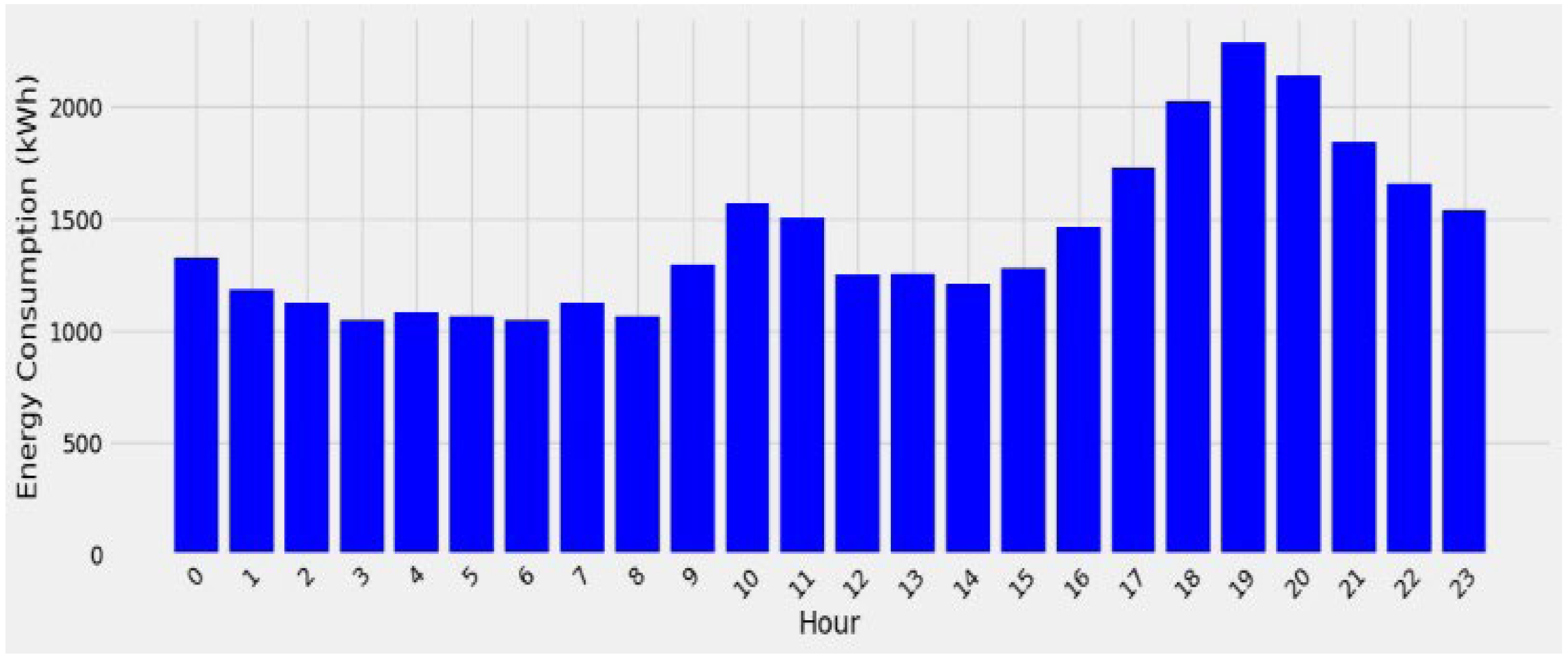
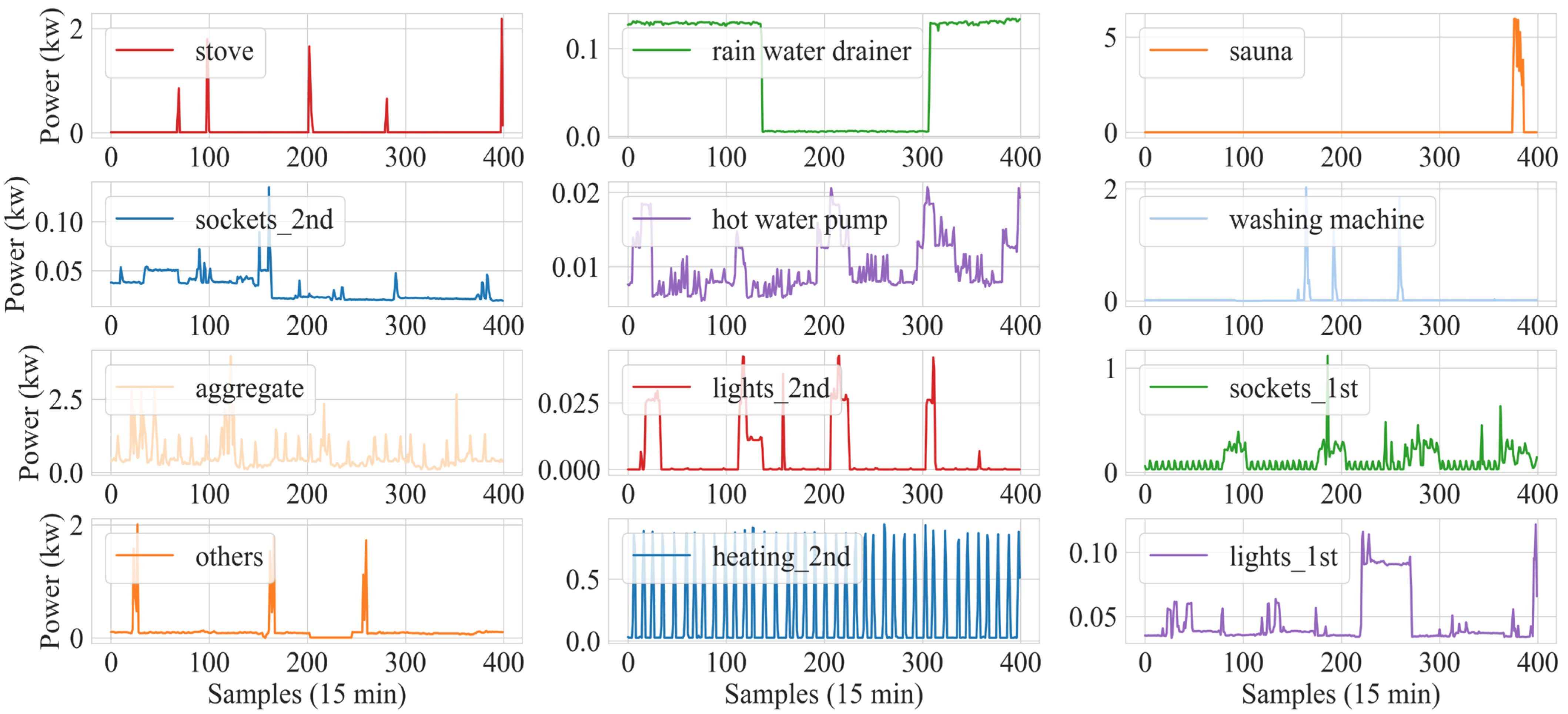
The hourly energy consumption data is presented in Figure 5 indicating the highest energy utilization during the evening hours around 7 and 8 p.m., coinciding with most occupants being at home. While there isn’t a specific hour of lowest energy consumption evident in the analysis, energy usage tends to be lower in the early morning hours between 2 to 6 a.m. In Figure 6, the individual load patterns of devices like stoves, rainwater drainers, sauna, sockets, water pumps, washing machines, lights and heating are shown during a single day. The sauna, washing machine, electric stove, heater, and water pump are the most energy-consuming loads when they are being utilized.

4.2. Development of NILM based Models

In this research, all compilation has been done utilizing Python 3.10, TensorFlow 2.10.1, and Scikit-Learn1.4.1, running on a desktop with Intel(R) Core (TM) i7-7700K 4.20 GHz CPU, NVIDIA GeForce GTX 1080 GPU and 32 GB DDR4 RAM. The XgBoost and LSTM models have been trained on a GPU, utilizing the CUDA toolkit version 12.4. However, the Logistic Regression and DTW_KNN models have been trained on a CPU.

Data preprocessing lays the groundwork for effective model training. In the initial data preparation phase, handling missing values is crucial. Mean imputation (replacing missing values with the mean of available data) or forward fill (propagating the last observed value) can be utilized as more general and potentially effective solutions to address missing values. These methods offer more flexibility in handling different types of missing data while preserving the integrity of the dataset. The train-test split, typically at 80/20 ratio ensures unbiased model assessment, additionally shuffling the data during splitting ensures randomness and prevents any inherited order from affecting model performance. It is worth noticing that shuffling the data is not performed when working with LSTM due to the sequential nature of the data. This process is omitted to maintain the integrity of the temporal relationships within the dataset, ensuring optimal performance of the LSTM model. The model specifications for different algorithms are given in

Table 2. Model specifications for different algorithms.

Logistic Regression	Solver: “lbfgs”, Penalty: “L2”, Class Weighted: “balanced”, Max_Iteration: 150, Data Shuffle: Yes.
DTW_KNN	Number of Neighbors: 5, Window Size: 150 min (10 samples), Sample Signal Length: 360, Data Shuffle: No.
XgBoost	Booster: “dart”, Device: “GPU”, eta: 0.5, Max Depth: 4, Min_Child_Depth: 1, Max_Delta_Step: 1, Sub Sample: 0.9, Sampling Method: “Subsample”, Objective: “Binary Logistic”, Evaluation Metrics: “log loss”, Early Stopping: 10, Data Shuffle: Yes.
LSTM	Layer 1: Units: 50, Number of Features: 11 Layer 2: Dense:1, Activation: “Sigmoid” Optimizer: “Adam”, Learning Rate: 0.0005, Epochs: 60, Batch size: 32, Early Stopping: 10, metrics: “Accuracy”, Loss: “Binary Cross Entropy”, Validation Split: 0.1, Class Weight: “Balanced”, Data Shuffle = No

.

Time-related features play a significant role in modeling. Extracting the hour of the day, time interval number (with 15 min resolution), day of the week, and month provides valuable context. Generating cosine and sine values for these above-mentioned features encodes cyclic behavior and enhances models’ ability to learn from data. Additionally labeling weekends and holidays provides further insights for predictive modeling. Manual labeling on/off state of appliances based on specific thresholds ensures that the model can learn the underlying patterns as these labels serve as our target variable for supervised learning.

Handling power consumption patterns, particularly for devices with consistent steady consumption, requires a method that effectively identifies meaningful deviations in power usage, filtering out noise and focusing on relevant changes. The approach involves establishing a baseline consumption level for devices such as sockets and lights, representing the minimal power draw when inactive. Significant increases in power consumption beyond this baseline are then interpreted as the device being turned on. Additionally, recognizing that certain devices may exhibit consistent consumption patterns, such as modems, allows for their exclusion to prevent false positives. Overall, this approach balances sensitivity in detecting genuine “on” states with specificity in avoiding false positives, offering a practical means to enhance energy consumption prediction models.

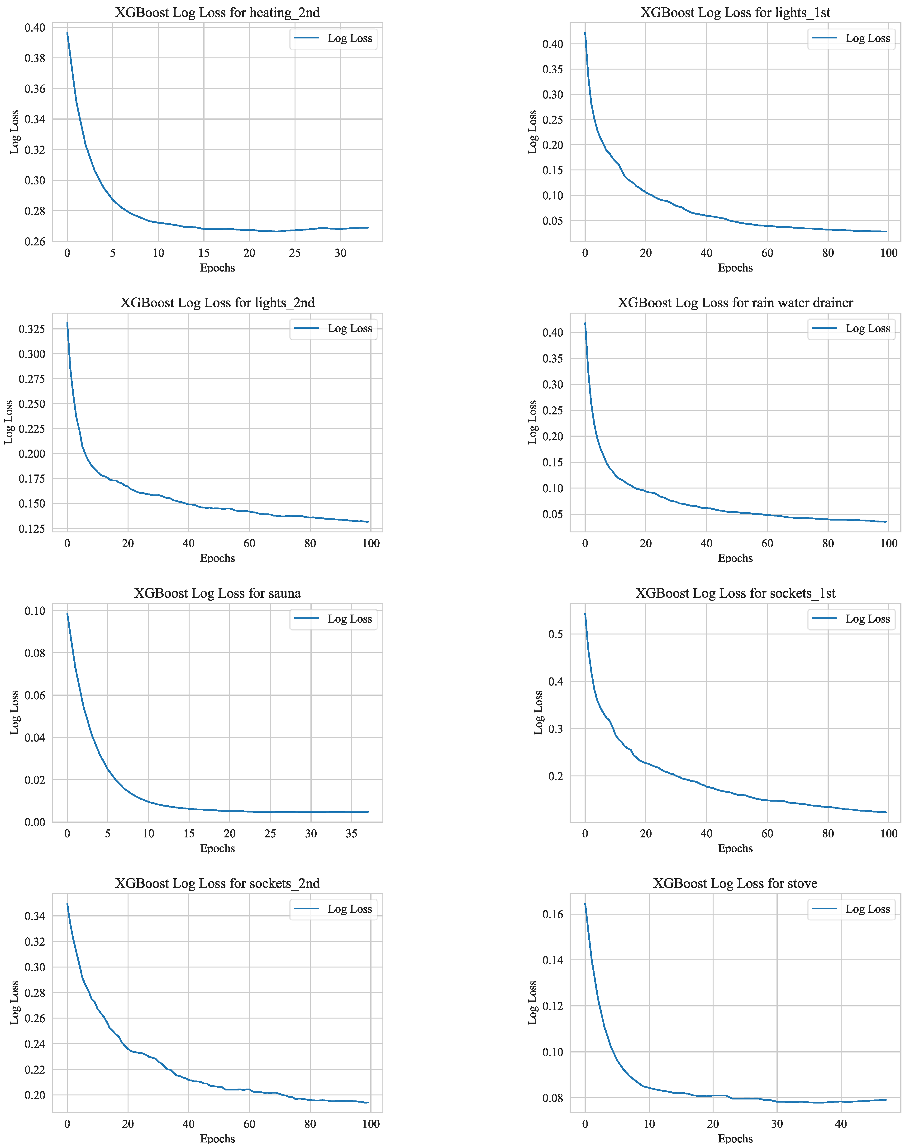
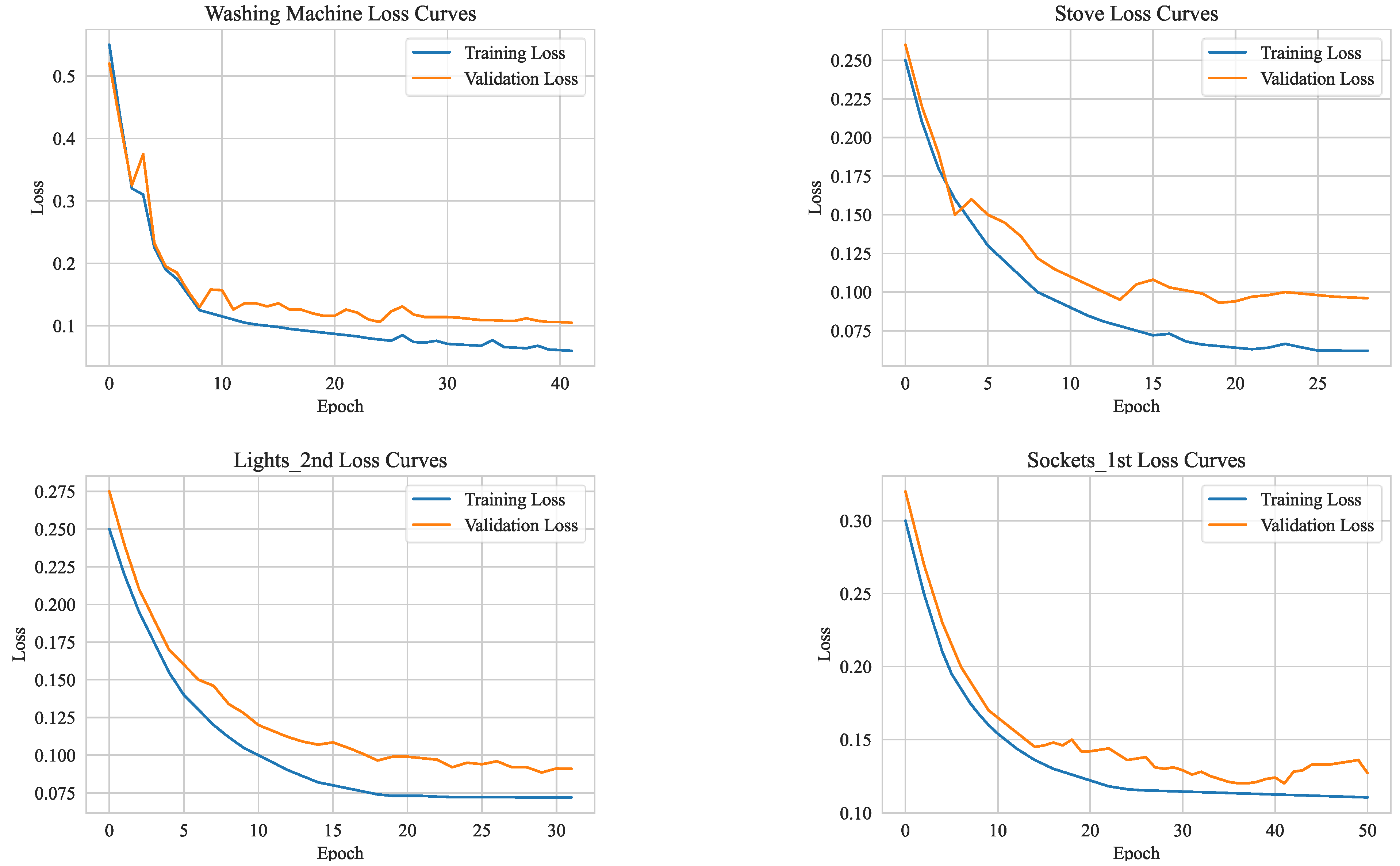
To avoid overfitting in our LSTM and XgBoost networks, we employ early stopping. This method halts the training when the model fails to improve on the validation data after several attempts. It monitors metrics such as loss or accuracy and terminates the training prematurely. This ensures that the model performs well with new data by stopping at the optimal moment. However, we acknowledge that including the training behavior of the models under investigation can offer additional insights into the design process. To this end, we have provided some examples related to the training procedures of LSTM and XgBoost networks below. Note that some of the training sessions ended before reaching the maximum epoch number due to the early stopping callback. Figure 7 shows the logarithmic loss curves related to XgBoost. In Figure 8, the LSTM training and validation losses are depicted.

5. Results and Discussion

As previously mentioned, our data comprise a 1-year aggregated record of electricity demand, including both the overall demand and the demands and consumption patterns of each appliance, with a resolution of 15 min. Consequently, the dataset encompasses approximately 35,000 data measurements for each sample. We have allocated 80% of the data for training and validation, and 20% for testing purposes. It is critical to highlight that we selected a 1-year period to capture all fluctuations related to seasonality. For example, the sauna is mostly used during the colder seasons, while during summer, the dataset records very few instances of sauna usage. This pattern holds true for heating systems as well.

As you truly mentioned a training time and resource usage investigation is also very important to make a fair comparison among proposed methods. To this end, the training time and RAM resource usage for all the models have been provided in

Table 3. Comparison of computation cost training times.

Appliance Name	Method	RAM Usage	Training Time Duration
Stove	LSTM	652 MB	104.62 s
	XgBoost	13.27 MB	2.58 s
	Logistic Regression	17 MB	0.156 s
Sockets_2nd	LSTM	456 MB	228.74 s
	XgBoost	4.6 MB	8.07 s
	Logistic Regression	0.87 MB	0.027 s
Heating_2nd	LSTM	381 MB	141.05 s
	XgBoost	5.65 MB	3.97 s
	Logistic Regression	1.12 MB	0.053 s
Washing Machine	LSTM	506 MB	288.38 s
	XgBoost	43 MB	7.84 s
	Logistic Regression	1.6 MB	0.16 s
Rainwater Drainer	LSTM	602 MB	289.56 s
	XgBoost	13.12 MB	7.31 s
	Logistic Regression	1.15 MB	0.047 s
Sockets_1st	LSTM	925 MB	169.72 s
	XgBoost	60 MB	6.86 s
	Logistic Regression	450 KB	0.05 s
Lights_1st	LSTM	319 MB	160.30 s
	XgBoost	73 MB	7.24 s
	Logistic Regression	626 KB	0.054 s
Sauna	LSTM	113 MB	131.14 s
	XgBoost	27 MB	1.11 s
	Logistic Regression	11 MB	0.027 s
Lights_2nd	LSTM	168 MB	87.52 s
	XgBoost	65 MB	7.37 s
	Logistic Regression	328 KB	0.036 s
Hot Water pump	LSTM	226 MB	165.17 s
	XgBoost	32 MB	2.26 s
	Logistic Regression	10.6 MB	0.16 s

.

The XgBoost algorithm stands out with exceptional performance across most cases, except for the “other” labeled group, which likely encompasses aggregated power consumption or unknown loads. Given its consistent performance, XgBoost emerges as a robust choice for the given task. The logistic regression demonstrates varying success rates, achieving optimal results in detecting sauna status and rainwater drainers but faltering in other cases.

Dynamic time warping with K-nearest neighbors segments consumption curves into 400-length samples, employing a warping window size of 10 samples to determine appliance classes based on the five nearest neighbors. While generally effective, misidentifications between appliances like washing machines and stoves indicate room for improvement—perhaps through refined feature engineering. Additionally, mislabeling lights_1st and lights_2nd as “others” due to their similar patterns underscores the method’s susceptibility to mixing closely related patterns.

By exploiting the LSTM architecture to analyze 480 samples, representing a window spanning 120 h, the model effectively captures temporal dependencies and inherent patterns within the dataset. The strategic handling of imbalanced labels through the implementation of the class weight method reflects a judicious approach to mitigate bias during model training. The adjustment of class weights ensures equitable consideration of both “on” and “off” states, thereby averting the model’s inclination towards the predominant class and fostering a more balanced learning process.

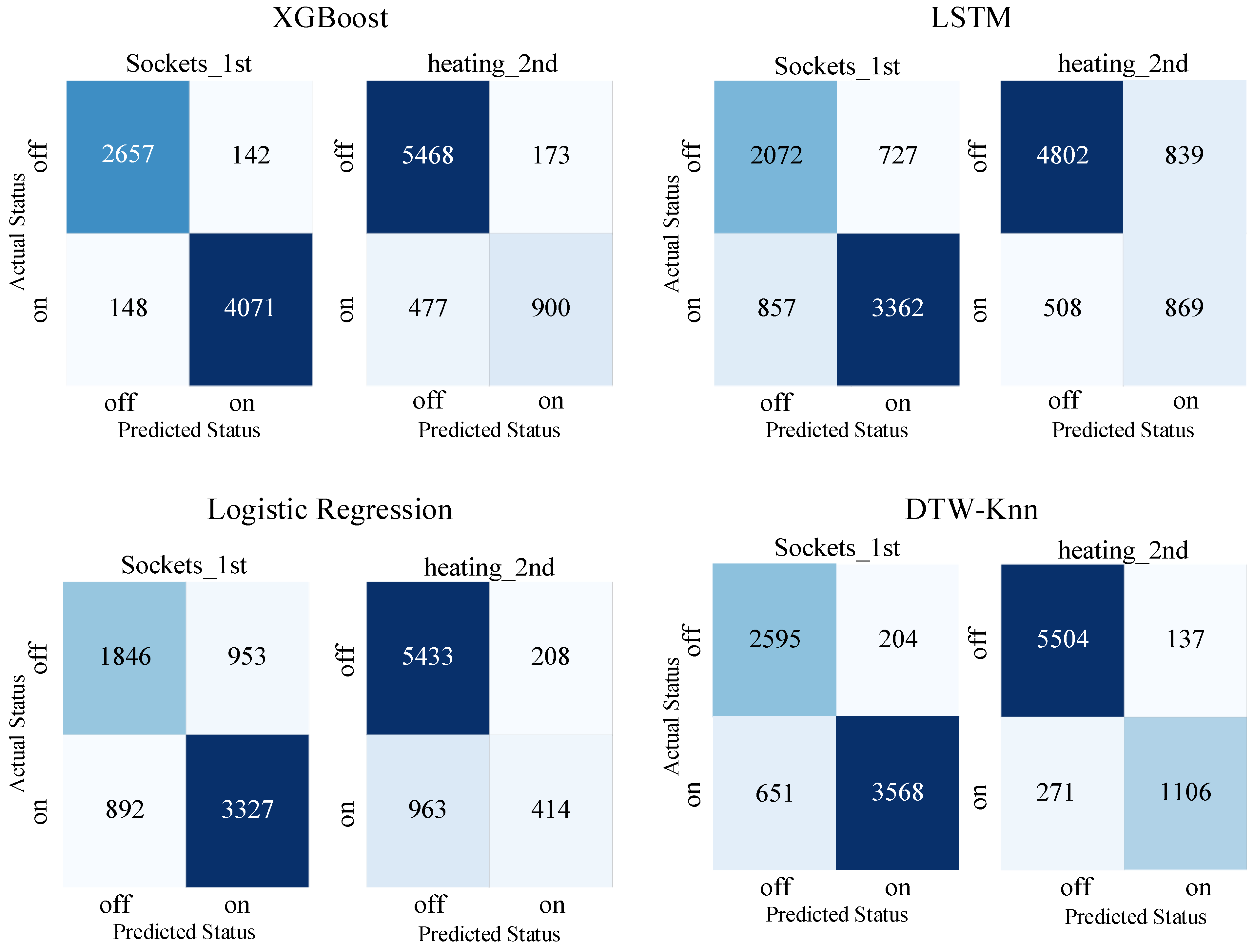
In the domain of NILM, the classification threshold plays a pivotal role in optimizing the balance between precision and recall. Precision, prioritizing correctness, and risks overlook certain energy consumption patterns, while recall, emphasizing completeness may falsely identify non-existent appliance activations. The choice to adjust the threshold depends on the consequences within the context of energy management. For instance, in residential energy monitoring, minimizing false negatives is crucial to accurately detect appliance usage, ensuring efficient energy usage and potentially identifying malfunctioning devices. Conversely, in commercial settings like smart buildings, reducing false positives is essential to avoid unnecessary interventions and maintain occupants’ comfort while optimizing energy consumption.

In the provided Figure 9 the confusion matrices indicate that the LSTM method performed less effectively compared to other techniques. One possible reason for this discrepancy could be the suboptimal sampling rate of 15 min. Previous studies have shown that increasing the measurement frequency can significantly enhance prediction accuracy in NILM applications. Additionally, fine-tuning the LSTM method through architectural adjustments or hyperparameter tuning may further improve its performance. Therefore, future research should explore optimizing the sampling frequency alongside other methodological enhancements to maximize the effectiveness of LSTM-based NILM approaches.

However, comparative analyses (see

Table 4. Performance analysis of different ML algorithms.

Appliance	Stove			Washing Machine			Sauna
Model Metrics	Precision	Recall	F1-Scroe	Precision	Recall	F1-Scroe	Precision	Recall	F1-Scroe
DTW_KNN	0.91	0.92	0.95	0.86	0.48	0.62	0.92	0.79	0.85
XgBoost	0.87	0.73	0.78	0.87	0.74	0.79	0.94	0.93	0.93
LR	0.71	0.56	0.59	0.72	0.56	0.59	0.95	0.92	0.93
LSTM	0.63	0.95	0.69	0.58	0.92	0.63	0.76	1.00	0.84
Appliance	Heating_2nd			Sockets_2nd			Rainwater drainer
Model Metrics	Precision	Recall	F1-scroe	Precision	Recall	F1-scroe	Precision	Recall	F1-scroe
DTW_KNN	0.91	1.00	0.95	0.94	0.83	0.88	1.00	0.95	0.97
XgBoost	0.90	0.91	0.90	0.87	0.75	0.79	0.99	0.99	0.99
LR	0.81	0.83	0.81	0.81	0.88	0.82	0.86	0.86	0.85
LSTM	0.90	0.89	0.89	0.96	0.92	0.94	0.93	0.96	0.95
Appliance	Sockets_1st			Lights_1st			Hot water pump
Model Metrics	Precision	Recall	F1-scroe	Precision	Recall	F1-scroe	Precision	Recall	F1-scroe
DTW_KNN	0.92	0.79	0.85	0.94	0.60	0.73	0.80	0.92	0.86
XgBoost	0.96	0.96	0.96	0.99	0.98	0.99	0.85	0.88	0.89
LR	0.74	0.74	0.74	0.77	0.79	0.76	0.70	0.71	0.70
LSTM	0.83	0.81	0.82	0.82	0.73	0.76	0.60	1.00	0.66
Appliance	Lights_2nd			Others			Total Performance
Model Metrics	Precision	Recall	F1-scroe	Precision	Recall	F1-scroe	Precision	Recall	F1-scroe
DTW_KNN	0.90	0.82	0.82	0.52	1.00	0.68	0.93	0.85	0.86
XgBoost	0.92	0.90	0.91	0.80	0.67	0.71	0.91	0.86	0.88
LR	0.86	0.88	0.87	0.95	0.97	0.96	0.81	0.79	0.78
LSTM	0.96	0.86	0.90	0.70	0.81	0.75	0.79	0.90	0.80

) reveal that alternative models such as XgBoost and DTW with KNN outperform LSTM in the specific scenario under investigation, emphasizing the importance of exploring diverse model architectures and methodologies. Considerations of interpretability, computational efficiency, and ease of implementation will be pivotal in inappropriate model selection for a given task.

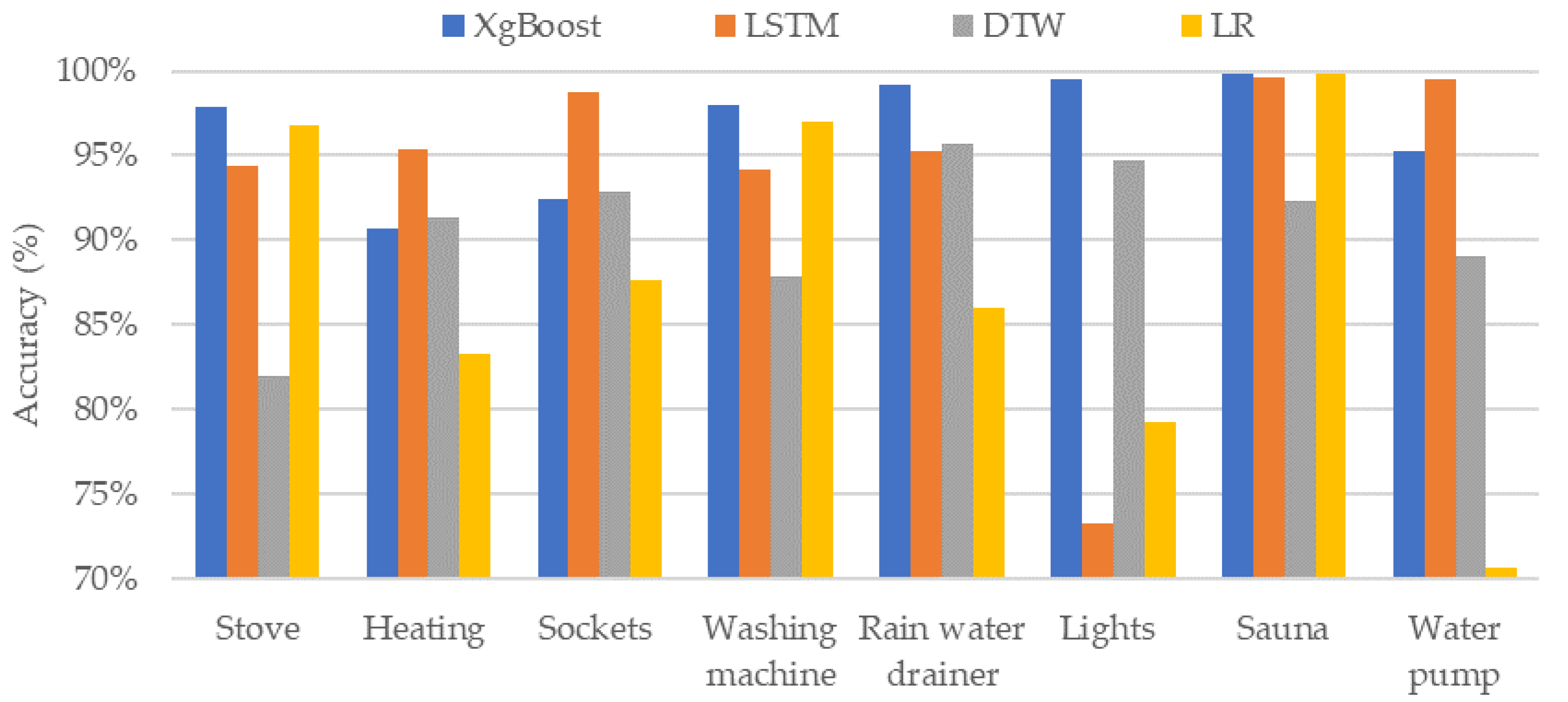
Figure 10 depicts the comparative analysis of all the ML algorithms based on the accuracy of identification of the appliance at the individual level. The accuracy of LSTM and XgBoost is comparable for most of the devices, however, the accuracy of LSTM is extremely low for the lighting loads. On the other side, the LR algorithm has low accurate results for lights, heating, and rainwater drainer. The DTW-KNN algorithm shows comparatively better results than the LR algorithm, but it also has variations in accuracy results. Overall, the most consistent results are from the XgBoost algorithm.

There could be several reasons why XgBoost outperforms other methods. First, XgBoost effectively handles various data types and missing values, which can be beneficial when dealing with different sampling rates. In our case, the sampling rate was quite low. On the other hand, LSTM can be significantly influenced by the sampling rate. Additionally, the amount of training data has a substantial impact on the performance of neural networks due to their long-term memory capability. Sampling rates matter in Logistic Regression as well. Secondly, XgBoost, as a representative of the family of gradient boosting algorithms, is more robust to overfitting compared to deep learning models like LSTM. This could be particularly beneficial if the data set is not very large, as in our case. XgBoost has many parameters, which gives the designer the opportunity to tune the model and prevent overfitting.

In general, all algorithms have their strengths and weaknesses. For instance, LSTM has the ability to capture long-term dependencies, but it may require a large amount of data and computational resources. Logistic Regression is a simple and fast algorithm, but it may not capture complex patterns in the data. DTW-KNN is good at capturing temporal patterns, but it may be sensitive to noise and outliers. All of the above leads to the conclusion that it is reasonable to focus on developing hybrid models that combine the strengths of different algorithms. Moreover, improving the robustness and efficiency of existing algorithms is valuable as well. This approach not only enhances the performance of the model but also makes it more adaptable to various types of data and tasks.

6. Conclusions

As energy consumption monitoring becomes increasingly vital in the transition towards sustainable practices, this research provides valuable guidance for the selection and deployment of ML techniques in Non-Intrusive Load Monitoring systems. This paper presents a thorough analysis of machine learning techniques employed by NILM through a meticulous examination and comparison, we have elucidated the efficacy and adaptability of various algorithms in disaggregating energy consumption data accurately. Our research underscores the necessity of tailored approaches, emphasizing the significance of selecting suitable models aligned with the specific characteristics and objectives of the data at hand. By providing a nuanced understanding of the strengths and limitations inherent in different methodologies, our study offers valuable insights that can inform the development and implementation of more efficient NILM systems. Furthermore, our findings highlight the multifaceted nature of NILM challenges and the complexity involved in accurately discerning individual appliance signatures from aggregate energy data. The results of this study indicate that the LSTM and XgBoost algorithms give the most accurate identification results, however, XgBoost has the best results on average.

Looking ahead, as the field of NILM continues to evolve, further research and innovation are warranted to address persistent challenges and capitalize on emerging opportunities. By fostering interdisciplinary collaborations and leveraging advances in data science, artificial intelligence, and energy engineering, we can unlock new avenues for improving the accuracy, efficiency, and scalability of NILM solutions. Ultimately, our collective efforts aim to empower consumers with actionable insights, facilitate informed decision-making, and promote sustainable energy consumption practices in support of a more resilient and environmentally conscious future.

References

- Ji, X.; Huang, H.; Chen, D.; Yin, K.; Zuo, Y.; Chen, Z.; Bai, R. A Hybrid Residential Short-Term Load Forecasting Method Using Attention Mechanism and Deep Learning. Buildings 2023, 13, 72. [Google Scholar] [CrossRef]
- Jawad, M.; Asghar, H.; Arshad, J.; Javed, A.; Qureshi, M.B.; Ali, S.M.; Shabbir, N.; Rassõlkin, A. A Novel Renewable Powered Stand-Alone Electric Vehicle Parking-Lot Model. Sustain. Energy Grids Netw. 2023, 33, 100992. [Google Scholar] [CrossRef]
- Mirza, Z.T.; Anderson, T.; Seadon, J.; Brent, A. A thematic analysis of the factors that influence the development of a renewable energy policy. Renew. Energy Focus 2024, 49, 100562. [Google Scholar] [CrossRef]
- Abumohsen, M.; Owda, A.Y.; Owda, M. Electrical Load Forecasting Using LSTM, GRU, and RNN Algorithms. Energies 2023, 16, 2283. [Google Scholar] [CrossRef]
- Azizi, E.; Ahmadiahangar, R.; Rosin, A.; Bolouki, S. Characterizing Energy Flexibility of Buildings with Electric Vehicles and Shiftable Appliances on Single Building Level and Aggregated Level. Sustain. Cities Soc. 2022, 84, 103999. [Google Scholar] [CrossRef]
- Azizi, E.; Shotorbani, A.M.; Hamidi-Beheshti, M.T.; Mohammadi-Ivatloo, B.; Bolouki, S. Residential Household Non-Intrusive Load Monitoring via Smart Event-Based Optimization. IEEE Trans. Consum. Electron. 2020, 66, 233–241. [Google Scholar] [CrossRef]
- Opoku, R.; Obeng, G.Y.; Adjei, E.A.; Davis, F.; Akuffo, F.O. Integrated System Efficiency in Reducing Redundancy and Promoting Residential Renewable Energy in Countries without Net-Metering: A Case Study of a SHS in Ghana. Renew. Energy 2020, 155, 65–78. [Google Scholar] [CrossRef]
- Azizi, E.; Beheshti, M.T.H.; Bolouki, S. Event Matching Classification Method for Non-Intrusive Load Monitoring. Sustainability 2021, 13, 693. [Google Scholar] [CrossRef]
- Lizana, J.; Friedrich, D.; Renaldi, R.; Chacartegui, R. Energy Flexible Building through Smart Demand-Side Management and Latent Heat Storage. Appl. Energy 2018, 230, 471–485. [Google Scholar] [CrossRef]
- Kaselimi, M.; Protopapadakis, E.; Voulodimos, A.; Doulamis, N.; Doulamis, A. Multi-Channel Recurrent Convolutional Neural Networks for Energy Disaggregation. IEEE Access 2019, 7, 81047–81056. [Google Scholar] [CrossRef]
- Schirmer, P.A.; Mporas, I. Non-Intrusive Load Monitoring: A Review. IEEE Trans. Smart Grid 2023, 14, 769–784. [Google Scholar] [CrossRef]
- Angelis, G.F.; Timplalexis, C.; Salamanis, A.I.; Krinidis, S.; Ioannidis, D.; Kehagias, D.; Tzovaras, D. Energformer: A New Transformer Model for Energy Disaggregation. IEEE Trans. Consum. Electron. 2023, 69, 308–320. [Google Scholar] [CrossRef]
- Azizi, E.; Beheshti, M.T.H.; Bolouki, S. Quantification of Disaggregation Difficulty with Respect to the Number of Smart Meters. IEEE Trans. Smart Grid 2022, 13, 516–525. [Google Scholar] [CrossRef]
- Shabbir, N.; Kutt, L.; Jawad, M.; Iqbal, M.N.; Ghahfarokhi, P.S. Forecasting of Energy Consumption and Production Using Recurrent Neural Networks. Adv. Electr. Electron. Eng. 2020, 18, 190–197. [Google Scholar] [CrossRef]
- Ding, G.; Wu, C.; Wang, Y.; Liang, Y.; Jiang, X.; Li, X. A Novel Non-Intrusive Load Monitoring Method Based on Quantum Particle Swarm Optimization Algorithm. In Proceedings of the 2019 11th International Conference on Measuring Technology and Mechatronics Automation (ICMTMA), Qiqihar, China, 28–29 April 2019; pp. 230–234. [Google Scholar] [CrossRef]
- Nuran, A.S.; Murti, M.A.; Suratman, F.Y. Non-Intrusive Load Monitoring Method for Appliance Identification Using Random Forest Algorithm. In Proceedings of the 2023 IEEE 13th Annual Computing and Communication Workshop and Conference (CCWC), Las Vegas, NV, USA, 8–11 March 2023; pp. 754–758. [Google Scholar] [CrossRef]
- Raiker, G.A.; Reddy, B.S.; Umanand, L.; Agrawal, S.; Thakur, A.S.; Ashwin, K.; Barton, J.P.; Thomson, M. Internet of Things Based Demand Side Energy Management System Using Non-Intrusive Load Monitoring. In Proceedings of the 2020 IEEE International Conference on Power Electronics, Smart Grid and Renewable Energy (PESGRE2020), Cochin, India, 2–4 January 2020; pp. 5–9. [Google Scholar] [CrossRef]
- Al-Khadher, O.; Mukhtaruddin, A.; Hashim, F.R.; Azizan, M.M.; Mamat, H.; Mani, M. Comparison of Non-Intrusive Load Monitoring Supervised Methods Using Harmonics as Feature. In Proceedings of the 2022 International Conference on Electrical, Computer and Energy Technologies (ICECET), Prague, Czech Republic, 20–22 July 2022; pp. 1–6. [Google Scholar] [CrossRef]
- Moradzadeh, A.; Zeinal-Kheiri, S.; Mohammadi-Ivatloo, B.; Abapour, M.; Anvari-Moghaddam, A. Support Vector Machine-Assisted Improvement Residential Load Disaggregation. In Proceedings of the 2020 28th Iranian conference on electrical engineering (ICEE), Tabriz, Iran, 4–6 August 2020; pp. 1–6. [Google Scholar] [CrossRef]
- Shiddieqy, H.A.; Hariadi, F.I.; Adijarto, W. Plug-Load Classification Based on CNN from V-I Trajectory Image Using STM32. In Proceedings of the 2021 International Symposium on Electronics and Smart Devices (ISESD), Bandung, Indonesia, 29–30 June 2021. [Google Scholar] [CrossRef]
- Giannuzzo, L.; Minuto, F.D.; Schiera, D.S.; Lanzini, A. Reconstructing Hourly Residential Electrical Load Profiles for Renewable Energy Communities Using Non-Intrusive Machine Learning Techniques. Energy AI 2024, 15, 100329. [Google Scholar] [CrossRef]
- Hernández, Á.; Nieto, R.; de Diego-Otón, L.; Pérez-Rubio, M.C.; Villadangos-Carrizo, J.M.; Pizarro, D.; Ureña, J. Detection of Anomalies in Daily Activities Using Data from Smart Meters. Sensors 2024, 24, 515. [Google Scholar] [CrossRef] [PubMed]
- Koasidis, K.; Marinakis, V.; Doukas, H.; Karamaneas, A.; Nikas, A.; Doumouras, N. Equipment- and Time-Constrained Data Acquisition Protocol for Non-Intrusive Appliance Load Monitoring. Energies 2023, 16, 7315. [Google Scholar] [CrossRef]
- Hosseini, S.S.; Delcroix, B.; Henao, N.; Agbossou, K.; Kelouwani, S. Towards Feasible Solutions for Load Monitoring in Quebec Residences. Sensors 2023, 23, 7288. [Google Scholar] [CrossRef] [PubMed]
- Shareef, H.; Asna, M.; Errouissi, R.; Prasanthi, A. Rule-Based Non-Intrusive Load Monitoring Using Steady-State Current Waveform Features. Sensors 2023, 23, 6926. [Google Scholar] [CrossRef]
- Azizi, E.; Beheshti, M.T.H.; Bolouki, S. Appliance-Level Anomaly Detection in Nonintrusive Load Monitoring via Power Consumption-Based Feature Analysis. IEEE Trans. Consum. Electron. 2021, 67, 363–371. [Google Scholar] [CrossRef]
- Welikala, S.; Dinesh, C.; Ekanayake, M.P.B.; Godaliyadda, R.I.; Ekanayake, J. Incorporating Appliance Usage Patterns for Non-Intrusive Load Monitoring and Load Forecasting. IEEE Trans. Smart Grid 2019, 10, 448–461. [Google Scholar] [CrossRef]
- Tao, Y.; Qiu, J.; Lai, S.; Wang, Y.; Sun, X. Reserve Evaluation and Energy Management of Micro-Grids in Joint Electricity Markets Based on Non-Intrusive Load Monitoring. IEEE Trans. Ind. Appl. 2023, 59, 207–219. [Google Scholar] [CrossRef]
- Ma, C.; Yin, L. Deep Flexible Transmitter Networks for Non-Intrusive Load Monitoring of Power Distribution Networks. IEEE Access 2021, 9, 107424–107436. [Google Scholar] [CrossRef]
- Garcia, F.D.; Souza, W.A.; Diniz, I.S.; Marafão, F.P. NILM-Based Approach for Energy Efficiency Assessment of Household Appliances. Energy Inform. 2020, 3, 10. [Google Scholar] [CrossRef]
- Liu, H.; Wu, H.; Yu, C. A Hybrid Model for Appliance Classification Based on Time Series Features. Energy Build. 2019, 196, 112–123. [Google Scholar] [CrossRef]
- Gopinath, R.; Kumar, M.; Prakash Chandra Joshua, C.; Srinivas, K. Energy Management Using Non-Intrusive Load Monitoring Techniques—State-of-the-Art and Future Research Directions. Sustain. Cities Soc. 2020, 62, 102411. [Google Scholar] [CrossRef]
- Du, Z.; Yin, B.; Zhu, Y.; Huang, X.; Xu, J. A NILM Load Identification Method Based on Structured V-I Mapping. Sci. Rep. 2023, 13, 21276. [Google Scholar] [CrossRef]
- Reddy, R.; Garg, V.; Pudi, V. A Feature Fusion Technique for Improved Non-Intrusive Load Monitoring. Energy Inform. 2020, 3, 9. [Google Scholar] [CrossRef]
- Ruano, A.; Hernandez, A.; Ureña, J.; Ruano, M.; Garcia, J. NILM Techniques for Intelligent Home Energy Management and Ambient Assisted Living: A Review. Energies 2019, 12, 2203. [Google Scholar] [CrossRef]
- Chen, T.; Guestrin, C. XGBoost: A Scalable Tree Boosting System. In Proceedings of the 22nd Acm Sigkdd International Conference on Knowledge Discovery and Data Mining, San Francisco, CA, USA, 13–17 August 2016; pp. 785–794. [Google Scholar] [CrossRef]
- He, K.; Stankovic, V.; Stankovic, L. Building a Graph Signal Processing Model Using Dynamic Time Warping for Load Disaggregation. Sensors 2020, 20, 6628. [Google Scholar] [CrossRef]
- Shabbir, N.; Ahmadiahangar, R.; Rosin, A.; Astapov, V.; Kilter, J. Short-Term PV Energy Generation Forecasting Using Deep Learning. Telematique 2022, 21, 5844–5850. [Google Scholar]
- Wang, R.; Tao, D. DTW-KNN Implementation for Touch-Based Authentication System. In Proceedings of the 2019 5th International Conference on Big Data Computing and Communications (BIGCOM), QingDao, China, 9–11 August 2019; pp. 318–322. [Google Scholar] [CrossRef]
- Feng, Z.; Wang, M.; He, J.; Xiao, W. Real-Time Equipment State Monitoring and Cycle Time Calculation Method Based on DTW-KNN. In Proceedings of the 2023 8th International Conference on Intelligent Computing and Signal Processing (ICSP), Xi’an, China, 21–23 April 2023; pp. 1350–1353. [Google Scholar] [CrossRef]
- Angelis, G.F.; Timplalexis, C.; Krinidis, S.; Ioannidis, D.; Tzovaras, D. NILM Applications: Literature Review of Learning Approaches, Recent Developments and Challenges. Energy Build. 2022, 261, 111951. [Google Scholar] [CrossRef]
- Imtiaz, M.A.; Raja, G. Isolated Word Automatic Speech Recognition (ASR) System Using MFCC, DTW & KNN. In Proceedings of the 2016 Asia Pacific Conference on Multimedia and Broadcasting (APMediaCast), Bali, Indonesia, 17–19 November 2017; pp. 106–110. [Google Scholar] [CrossRef]
- Yang, N.C.; Sung, K.L. Non-Intrusive Load Classification and Recognition Using Soft-Voting Ensemble Learning Algorithm with Decision Tree, K-Nearest Neighbor Algorithm and Multilayer Perceptron. IEEE Access 2023, 11, 94506–94520. [Google Scholar] [CrossRef]
- Shabbir, N.; Ahmadiahangar, R.; Rosin, A.; Jawad, M.; Kilter, J.; Martins, J. XgBoost Based Short-Term Electrical Load Forecasting Considering Trends & Periodicity in Historical Data. In Proceedings of the 2023 IEEE International Conference on Energy Technologies for Future Grids (ETFG), Wollongong, Australia, 3–6 December 2023; pp. 1–6. [Google Scholar] [CrossRef]
- Chen, Z.; Chen, J.; Xu, X.; Peng, S.; Xiao, J.; Qiao, H. Non-Intrusive Load Monitoring Based on Feature Extraction of Change-Point and Xgboost Classifier. In Proceedings of the 2020 IEEE 4th Conference on Energy Internet and Energy System Integration (EI2), Wuhan, China, 30 October–November 2020; pp. 2652–2656. [Google Scholar] [CrossRef]
- Semmelmann, L.; Henni, S.; Weinhardt, C. Load Forecasting for Energy Communities: A Novel LSTM-XGBoost Hybrid Model Based on Smart Meter Data. Energy Inform. 2022, 5, 24. [Google Scholar] [CrossRef]
- Mo, H.; Sun, H.; Liu, J.; Wei, S. Developing Window Behavior Models for Residential Buildings Using XGBoost Algorithm. Energy Build. 2019, 205, 109564. [Google Scholar] [CrossRef]
- Bipin Nair, B.J.; Yadhukrishnan, S.; Manish, A. A Comparative Study on Document Images Classification Using Logistic Regression and Multiple Linear Regressions. In Proceedings of the 2023 Second International Conference on Augmented Intelligence and Sustainable Systems (ICAISS), Trichy, India, 23–25 August 2023; pp. 1096–1104. [Google Scholar] [CrossRef]
- Shabbir, N.; Kütt, L.; Jawad, M.; Husev, O.; Rehman, A.U.; Gardezi, A.A.; Shafiq, M.; Choi, J.G. Short-Term Wind Energy Forecasting Using Deep Learning-Based Predictive Analytics. Comput. Mater. Contin. 2022, 72, 1017–1033. [Google Scholar] [CrossRef]
- Shabbir, N.; Kutt, L.; Raja, H.A.; Ahmadiahangar, R.; Rosin, A.; Husev, O. Machine Learning and Deep Learning Techniques for Residential Load Forecasting: A Comparative Analysis. In Proceedings of the IEEE 62nd International Scientific Conference on Power and Electrical Engineering of Riga Technical University, Riga, Latvia, 15–17 November 2021; pp. 1–5. [Google Scholar]
- Mellit, A.; Pavan, A.M.; Lughi, V. Deep Learning Neural Networks for Short-Term Photovoltaic Power Forecasting. Renew. Energy 2021, 172, 276–288. [Google Scholar] [CrossRef]
- Hossen, T.; Nair, A.S.; Chinnathambi, R.A.; Ranganathan, P. Residential Load Forecasting Using Deep Neural Networks (DNN). In Proceedings of the 2018 North American Power Symposium (NAPS), Fargo, ND, USA, 9–11 September 2019. [Google Scholar] [CrossRef]
- Shabbir, N.; Ahmadiahangar, R.; Rosin, A.; Husev, O.; Jalakas, T.; Martins, J. Residential DC Load Forecasting Using Long Short-Term Memory Network (LSTM). In Proceedings of the 2023 IEEE 11th International Conference on Smart Energy Grid Engineering (SEGE), Oshawa, ON, Canada, 13–15 August 2023; pp. 131–136. [Google Scholar] [CrossRef]