On the Regularization of Recursive Least-Squares Adaptive Algorithms Using Line Search Methods

Abstract

Stereophonic acoustic echo cancellation (SAEC) requires the identification of four unknown impulse responses corresponding to four loudspeaker-to-microphone pairs. Recent developments in the field of adaptive filters for SAEC setups have allowed for the handling of a single complex-valued adaptive impulse response, instead of the four classical real-valued adaptive filters. With the simplified framework provided by the widely linear (WL) model, more advanced versions of recursive least-squares (RLS) were employed in order to take advantage of their superior tracking speeds when working with highly correlated input signals (such as speech). Despite the performances and numerical stability provided by using exponentially weighted versions of the RLS family in combination with line search methods (LSMs), the SAEC configurations have limited capabilities in mitigating the negative effects caused by high-level disturbances affecting the two microphone signals. Such is the case of double-talk scenarios, which considerably reduce the update accuracy of the adaptive system. This paper analyzes a regularization technique for the named WL-RLS-LSM adaptive filters by adjusting the correlation matrix associated with the input signals and creating a reaction in the update process. The proposed method is designed to considerably slow (or even freeze) the adaptation process while the disturbance is manifested. Simulation results are discussed in order to validate the theoretical content.

1. Introduction

In the telecommunications domain, every audio terminal is equipped with a number of M microphones and L loudspeakers. When aiming to create the sensation of acoustic directionality, the values of M, respectively of L, are higher than 1. Correspondingly, every loudspeaker-to-microphone pair can form an undesired acoustic echo path and generate an associated acoustic echo signal [1,2,3,4]. The stereophonic configuration is obtained when employing the configuration $M=L=2$, and $M\times L=4$ unknown impulse responses must be estimated using four adaptive filters in order to cancel the effects of the associated echo signals [5,6,7,8,9,10].

In [2,6,11], the stereophonic acoustic echo cancellation (SAEC) problem was recast using the widely linear (WL) model, and the four adaptive filters were combined into a single adaptive impulse response with complex-valued coefficients. The WL framework maintains the same overall arithmetic effort and performance, with respect to the classical approach. Moreover, the new model can be applied to both the least-mean-square (LMS), respectively the recursive least-squares (RLS), families of adaptive algorithms [6,12,13,14].

From a practical point of view, SAEC applications have to manage hundreds or thousands of filter coefficients. Correspondingly, the convenient solution for the associated system identification problems is the LMS methods, which have poor performance when working with highly correlated input signals (e.g., with speech) [6,15,16,17,18]. As an alternative, the RLS methods have been the subject of ample research efforts because they can reduce the mentioned correlation problem and generate superior results. However, most RLS versions generate a direct solution for a system of N equations by using a complexity proportional to $\mathcal{O}\left(N^3\right)$ (in terms of multiplications), where N is the length of the associated adaptive filter. The approach is prohibitive for most modern chips. Even when applying less complex solutions to decrease the arithmetic workload, such as the one based on the matrix inversion lemma or the fast-RLS algorithm (complexities of $\mathcal{O}\left(N^2\right)$, respectively $\mathcal{O}\left(N\right)$), they tend to have numerical stability issues proportional to the reduction that is applied on the complexity side [6,12].

An alternative approach for the RLS adaptive algorithms with direct estimation of coefficients is to exploit the statistical properties of the input signal and replace the mentioned system of equations with an auxiliary system, which can be solved using iterative methods [2,19,20,21,22]. The result determined at each filter iteration is added to the previous filter estimate in order to generate the newest set of coefficients [19]. The approach is convenient for employing various line search methods (LSMs), which comprise several arithmetically efficient versions well suited for processing systems of equations specific to the complex-valued RLS adaptive algorithms [13].

Despite the fact that the named WL-RLS-LSM adaptive algorithms do not manifest numerical stability issues and are attractive for SAEC practical applications, they manifest the same vulnerabilities in high-noise or double-talk (DT) scenarios [23,24,25,26,27,28,29,30]. In such occurrences, the microphone signals are affected by other speech signals, and the update process of the complex-valued adaptive filter loses most of its accuracy. This paper studies a variable regularization (VR) technique for the RLS-specific correlation matrix designed to slow down or freeze the update operation [31,32]. We combine the mentioned regularization method with several complex-valued LSM alternatives, and we analyze the resulting algorithms from several points of interest: tracking speeds, accuracy at steady state, and efficiency in DT scenarios, respectively, and arithmetic complexity.

Traditional approaches require performing DT detection (DTD) on the four adaptive filters, estimating the four unknown impulse responses. The corresponding process of slowing down (or freezing) the update process of the coefficients depends on four associated indicators and can affect the performances of the entire mechanism. By interpreting the four adaptive filters as a single complex-valued filter, the decision is simplified, and the methodology can be focused on the efficiency of fewer decision indicators and parameters (e.g., thresholds, etc.). Consequently, for the case of the WL-RLS-LSM adaptive systems, the VR methodology is applied for a single correlation matrix instead of four such matrices.

The paper is organized as follows. Section 2 describes the system model corresponding to the SAEC setup working with RLS adaptive algorithms employing LSMs. In Section 3, the principle of the variable regularized RLS-LSM methods working within the WL framework is discussed. Section 4 presents several LSMs by taking into consideration the associated arithmetic complexities, and Section 5 analyzes the simulation results with the associated compromises between performances and complexity. Several conclusions are drawn in Section 6 regarding the possible practical applications of the WL-RLS-LSM family of adaptive algorithms.

2. System Model

This section describes the SAEC configuration using the WL model with respect to its corresponding particularities for the complex-valued RLS family of adaptive methods. To this purpose, the basic notation and the main relations that define the WL framework for SAEC from [2,6] are briefly described in this section, summarizing the required background for the upcoming developments. Moreover, using the simplified handling provided by the WL model, the exponentially weighted RLS adaptive algorithm using LSMs (i.e., the WL-RLS-LSM) is presented for solving the corresponding system of equations. The arithmetic workloads are also discussed.

2.1. The Widely-Linear Model

For the SAEC setup, the signals generated by the two loudspeakers represent the input information. We denote the discrete time index as n, and we write the corresponding acoustic signals by using $x_{{\mathrm{L}}_{\mathrm{c}}}\left(n\right)$ (for the left channel) and $x_{{\mathrm{R}}_{\mathrm{c}}}\left(n\right)$ (for the right channel). The WL model combines the two real-valued signals into a single complex-valued notation, and we write

$$\begin{array}{c}\hfill x\left(n\right)=x_{{\mathrm{L}}_{\mathrm{c}}}\left(n\right)+j{x}_{{\mathrm{R}}_{\mathrm{c}}}\left(n\right),\end{array}$$

(1)

where $j=\sqrt{-1}$ [6,11]. Correspondingly, we can express the two $N\times 1$ vectors comprising the last samples associated with the two acoustic channels as

$$\begin{array}{c}\hfill {\mathbf{x}}_{{\mathrm{L}}_{\mathrm{c}}}\left(n\right)={[x_{{\mathrm{L}}_{\mathrm{c}}}\left(n\right)x_{{\mathrm{L}}_{\mathrm{c}}}(n-1)\cdots x_{{\mathrm{L}}_{\mathrm{c}}}(n-N+1)]}^T,\end{array}$$

(2)

$$\begin{array}{c}\hfill {\mathbf{x}}_{{\mathrm{R}}_{\mathrm{c}}}\left(n\right)={[x_{{\mathrm{R}}_{\mathrm{c}}}\left(n\right)x_{{\mathrm{R}}_{\mathrm{c}}}(n-1)\cdots x_{{\mathrm{R}}_{\mathrm{c}}}(n-N+1)]}^T,\end{array}$$

(3)

where the superscript ^T represents the transpose operator. We can also cumulate all input information into a single $N\times 1$ complex-valued vector as

$$\begin{array}{c}\hfill \mathbf{x}\left(n\right)={\mathbf{x}}_{{\mathrm{L}}_{\mathrm{c}}}\left(n\right)+j{\mathbf{x}}_{{\mathrm{R}}_{\mathrm{c}}}\left(n\right).\end{array}$$

(4)

Furthermore, we denote the four $N\times 1$ impulse responses associated with the loudspeaker-to-microphone echo paths by using ${\mathbf{h}}_{\mathrm{t},{\mathrm{L}}_{\mathrm{c}}{\mathrm{L}}_{\mathrm{c}}}$, ${\mathbf{h}}_{\mathrm{t},{\mathrm{L}}_{\mathrm{c}}{\mathrm{R}}_{\mathrm{c}}}$, ${\mathbf{h}}_{\mathrm{t},{\mathrm{R}}_{\mathrm{c}}{\mathrm{L}}_{\mathrm{c}}}$ with ${\mathbf{h}}_{\mathrm{t},{\mathrm{R}}_{\mathrm{c}}{\mathrm{R}}_{\mathrm{c}}}$, respectively. The output samples corresponding to the left and right channels are obtained by employing the inputs in (2) and (3) [2,11] and writing

$$\begin{array}{c}\hfill y_{{\mathrm{L}}_{\mathrm{c}}}\left(n\right)={\mathbf{h}}_{\mathrm{t},{\mathrm{L}}_{\mathrm{c}}{\mathrm{L}}_{\mathrm{c}}}^T{\mathbf{x}}_{{\mathrm{L}}_{\mathrm{c}}}\left(n\right)+{\mathbf{h}}_{\mathrm{t},{\mathrm{R}}_{\mathrm{c}}{\mathrm{L}}_{\mathrm{c}}}^T{\mathbf{x}}_{{\mathrm{R}}_{\mathrm{c}}}\left(n\right),\end{array}$$

(5)

$$\begin{array}{c}\hfill y_{{\mathrm{R}}_{\mathrm{c}}}\left(n\right)={\mathbf{h}}_{\mathrm{t},{\mathrm{L}}_{\mathrm{c}}{\mathrm{R}}_{\mathrm{c}}}^T{\mathbf{x}}_{{\mathrm{L}}_{\mathrm{c}}}\left(n\right)+{\mathbf{h}}_{\mathrm{t},{\mathrm{R}}_{\mathrm{c}}{\mathrm{R}}_{\mathrm{c}}}^T{\mathbf{x}}_{{\mathrm{R}}_{\mathrm{c}}}\left(n\right),\end{array}$$

(6)

where we can also express a complex-valued output signal in the form of

$$\begin{array}{c}\hfill y\left(n\right)=y_{{\mathrm{L}}_{\mathrm{c}}}\left(n\right)+j{y}_{{\mathrm{R}}_{\mathrm{c}}}\left(n\right).\end{array}$$

(7)

The four real-valued acoustic impulse responses can be combined into two $N\times 1$ complex-valued systems

$$\begin{array}{cc}\hfill {\mathbf{h}}_{\alpha }& =\frac{{\mathbf{h}}_{\mathrm{t},{\mathrm{L}}_{\mathrm{c}}{\mathrm{L}}_{\mathrm{c}}}+{\mathbf{h}}_{\mathrm{t},{\mathrm{R}}_{\mathrm{c}}{\mathrm{R}}_{\mathrm{c}}}}{2}+j\frac{{\mathbf{h}}_{\mathrm{t},{\mathrm{R}}_{\mathrm{c}}{\mathrm{L}}_{\mathrm{c}}}-{\mathbf{h}}_{\mathrm{t},{\mathrm{L}}_{\mathrm{c}}{\mathrm{R}}_{\mathrm{c}}}}{2},\hfill \end{array}$$

(8)

$$\begin{array}{cc}\hfill {\mathbf{h}}_{\beta }& =\frac{{\mathbf{h}}_{\mathrm{t},{\mathrm{L}}_{\mathrm{c}}{\mathrm{L}}_{\mathrm{c}}}-{\mathrm{h}}_{\mathrm{t},{\mathrm{R}}_{\mathrm{c}}{\mathrm{R}}_{\mathrm{c}}}}{2}-j\frac{{\mathbf{h}}_{\mathrm{t},{\mathrm{R}}_{\mathrm{c}}{\mathrm{L}}_{\mathrm{c}}}+{\mathbf{h}}_{\mathrm{t},{\mathrm{L}}_{\mathrm{c}}{\mathrm{R}}_{\mathrm{c}}}}{2},\hfill \end{array}$$

(9)

and we introduce a single notation for handling all the real-valued loudspeaker-to-microphone echo paths in the form of a $2N\times 1$ complex-valued impulse response using the interleaving operation:

$$\begin{array}{c}\hfill {\mathbf{h}}_{\mathrm{t}}={\left[h_{\alpha ,0}{h}_{\beta ,0}\dots h_{\alpha ,N-1}{h}_{\beta ,N-1}\right]}^T,\end{array}$$

(10)

where $h_{\alpha ,l}$ and $h_{\beta ,l}$, with $l=0,1,\dots ,N-1$, are the elements of the vectors ${\mathbf{h}}_{\alpha }$ and ${\mathbf{h}}_{\beta }$, respectively [6].

The input information can also be arranged in a suitable manner by employing the interleaving operation. We write the $2N\times 1$ complex-valued vector

$$\begin{array}{c}\hfill {\mathbf{x}}_{\mathrm{in}}\left(n\right)={\left[x\left(n\right)x^{*}\left(n\right)\dots x(n-N+1)x^{*}(n-N+1)\right]}^T,\end{array}$$

(11)

and we can obtain a simpler expression for the complex output as

$$\begin{array}{c}\hfill y\left(n\right)={\mathbf{h}}_{\mathrm{t}}^H{\mathbf{x}}_{\mathrm{in}}\left(n\right).\end{array}$$

(12)

where ^H denotes the Hermitian operator [6].

With the improved handling provided by the WL model, we also write the complex reference signal as

$$\begin{array}{c}\hfill d\left(n\right)=y\left(n\right)+w\left(n\right),\end{array}$$

(13)

where $w\left(n\right)=w_{{\mathrm{L}}_{\mathrm{c}}}\left(n\right)+j{w}_{{\mathrm{R}}_{\mathrm{c}}}\left(n\right)$ represents the complex noise affecting the microphone channels. Its corresponding components (i.e., $w_{{\mathrm{L}}_{\mathrm{c}}}\left(n\right)$ and $w_{{\mathrm{R}}_{\mathrm{c}}}\left(n\right)$) are uncorrelated with the loudspeaker signals. Moreover, considering the complex estimate $\tilde{y}\left(n\right)$ generated by the SAEC system for the output $y\left(n\right)$, by employing a single adaptive filter, $\tilde{\mathbf{h}}\left(n\right)$, with $2N\times 1$ complex-valued coefficients, the a posteriori error can be defined as

$$\begin{array}{c}\hfill e\left(n\right)=d\left(n\right)-\tilde{y}\left(n\right)=d\left(n\right)-{\tilde{\mathbf{h}}}^H\left(n\right){\mathbf{x}}_{\mathrm{in}}\left(n\right).\end{array}$$

(14)

The described WL model simplifies the handling of the SAEC setup by employing the minimum possible number of notations for all the involved signals. Additionally, four unknown acoustic impulse responses, which would normally require four adaptive algorithms, are now combined into a single complex-valued system estimated using a single adaptive filter. The overall arithmetic complexity and the associated performances do not change [2,6].

2.2. The WL-RLS-LSM Algorithm

The exponentially weighted versions of the RLS adaptive methods are developed based on the cost function

$$\begin{array}{c}\hfill {\mathcal{J}}_{\mathrm{LS}}\left[\tilde{\mathbf{h}}\left(n\right)\right]=\sum _{i=1}^n{\lambda }^{n-i}{\left[d\left(i\right)-{\tilde{\mathbf{h}}}^H\left(n\right){\mathbf{x}}_{\mathrm{in}}\left(i\right)\right]}^2,\end{array}$$

(15)

where $0<\lambda \le 1$ denotes the forgetting factor [6,12]. The value of $\lambda$ is associated with a compromise made between the tracking capabilities of the algorithm, on one side, with respect to the accuracy it has at steady state on the other side. For lower values of $\lambda$, the memory of the algorithm is diminished, and the contributions associated with older information become negligibly faster. In such cases, the algorithm adapts faster to any changes that might occur in the unknown system to be identified. When the value of $\lambda$ is closer to 1 (i.e., to infinite memory), the tracking of changes is slower. However, more information about loudspeakers and the respective microphone signals is stored at once. Thus, the accuracy of the RLS is better under a steady state, and the misadjustment decreases [13]. We employ the forgetting factor and express the recursive notations

$$\begin{array}{cc}\hfill \mathbf{R}\left(n\right)& =\lambda \mathbf{R}(n-1)+{\mathbf{x}}_{\mathrm{in}}\left(n\right){\mathbf{x}}_{\mathrm{in}}^H\left(n\right),\hfill \end{array}$$

(16)

$$\begin{array}{cc}\hfill \mathbf{p}\left(n\right)& =\lambda \mathbf{p}(n-1)+{\mathbf{x}}_{\mathrm{in}}\left(n\right)d\left(n\right),\hfill \end{array}$$

(17)

where $\mathbf{R}\left(n\right)$ is the $2N\times 2N$ estimate of the correlation matrix associated with the complex input signal, and $\mathbf{p}\left(n\right)$ represents the $2N\times 1$ cross-correlation vector between the input signal and the complex reference, respectively [6,12]. Consequently, we can employ the notations mentioned above, and the minimization of the cost function in (15) leads to the system of equations

$$\begin{array}{cc}\hfill \mathbf{R}\left(n\right)\tilde{\mathbf{h}}\left(n\right)& =\mathbf{p}\left(n\right).\hfill \end{array}$$

(18)

The direct solution for (18) requires computing the inverse of the matrix $\mathbf{R}\left(n\right)$ at every time index, n. Such an approach is prohibitive for modern chips because the usual number of filter coefficients for SAEC applications is in the range of thousands. A popular alternative to the direct solution is the complex-valued RLS method based on the matrix inversion lemma (also known as Woodbury’s identity), which is often used as a reference for research work [12]. In the rest of the paper, we will call the mentioned algorithm the WL-RLS method. It requires a number of complex multiplications proportional to $4N^2$, as well as $4N$ real-valued divisions for every filter iteration. Despite the reduction in computational effort by an order of magnitude, the overall complexity is still considered difficult to approach for SAEC applications, which might also be affected by the associated numerical stability issues.

Fundamental research led to the reinterpretation of the system in (18) in order to exploit the statistical properties of the loudspeaker signals, as they are reflected in the correlation matrix $\mathbf{R}\left(n\right)$ [19,20,21]. Consequently, the exponentially weighted RLS methods can be combined with different LSM variants in order to solve an auxiliary system of equations. The resulting WL-RLS-LSM algorithms can provide performances comparable to the WL-RLS without manifesting numerical stability issues [2,19]. Several versions also have lower arithmetic complexities with respect to the WL-RLS. The steps of the WL-RLS-LSM general method are presented in

Table 1. WL-RLS-LSM Algorithm.

Step	Actions	×
	$\mathrm{Initialization}:$
	$\tilde{\mathbf{h}}\left(0\right)={\mathbf{0}}_{2N\times 1};$	0
	$\mathbf{r}\left(0\right)={\mathbf{0}}_{2N\times 1};$	0
	$\mathbf{R}\left(0\right)=\Phi {\mathbf{I}}_{2N},\Phi >0$	0
	$\mathrm{For}n=1,2,3\dots \dots$
1	Update ${\mathbf{x}}_{\mathrm{in}}\left(n\right)$ using (1) and (11)	0
2	Update $\mathbf{R}\left(n\right)$ using time-shift
	${\mathbf{R}}_{:,1}\left(n\right)=\lambda {\mathbf{R}}_{:,1}(n-1)+x^{*}\left(n\right){\mathbf{x}}_{\mathrm{in}}\left(n\right)$	$4N$
3	$\tilde{y}\left(n\right)={\tilde{\mathbf{h}}}^H(n-1){\mathbf{x}}_{\mathrm{in}}\left(n\right)$	$8N$
4	$e\left(n\right)=d\left(n\right)-\tilde{y}\left(n\right)$	0
5	${\mathbf{p}}_0\left(n\right)=\lambda \mathbf{r}(n-1)+e^{*}\left(n\right){\mathbf{x}}_{\mathrm{in}}\left(n\right)$	$4N$
6	$\mathbf{R}\left(n\right)\Delta \mathbf{h}\left(n\right)={\mathbf{p}}_0\left(n\right)\stackrel{\mathrm{LSM}}{\to }\Delta \tilde{\mathbf{h}}\left(n\right),\mathbf{r}\left(n\right)$	...
7	$\tilde{\mathbf{h}}\left(n\right)=\tilde{\mathbf{h}}(n-1)+\Delta \tilde{\mathbf{h}}\left(n\right)$	0

, where the corresponding amounts of necessary real-valued multiplications are also displayed.

The initialization stage runs once and employs the $2N\times 1$ zero-valued vector ${\mathbf{0}}_{2N\times 1}$ to set the values of the filter coefficients $\tilde{\mathbf{h}}\left(0\right)$ of the $2N\times 1$ residual vector, $\mathbf{r}\left(0\right)$. Moreover, the $2N\times 2N$ identity matrix ${\mathbf{I}}_{2N}$ is used to fill the correlation matrix estimate $\mathbf{R}\left(0\right)$ with zeroes on all positions, excepting the main diagonal, where the small, real-valued positive constant $\Phi$ is used to avoid the singular property in the initial stages of the algorithm. In the form presented in Table 1, the effect of $\Phi$ becomes negligible after the WL-RLS-LSM runs for a certain number of iterations due to the effect of the forgetting factor.

Steps 1 to 7 run each time for every time index n, and the first four stages are the same as the other exponentially weighted RLS methods working with complex values in the SAEC framework [6,11]. Steps 1 and 2 perform the update of the input vector ${\mathbf{x}}_{\mathrm{in}}\left(n\right)$ with respect to the correlation matrix $\mathbf{R}\left(n\right)$. Apparently, the computation of the latter using (16) requires an amount of multiplications proportional to the square of $2N$. However, the input vector has the $time$-$shift$ property and can be expressed as

$$\begin{array}{c}\hfill {\mathbf{x}}_{\mathrm{in}}\left(n\right)={\left[x\left(n\right)x^{*}\left(n\right){\mathbf{x}}_{\mathrm{in},1:2N-2}^T(n-1)\right]}^T,\end{array}$$

(19)

where ${\mathbf{x}}_{\mathrm{in},1:2N-2}(n-1)$ is the $(2N-2)\times 1$ vector comprising the last $2N-2$ complex-valued input samples from time index $n-1$. Correspondingly, $\mathbf{R}\left(n\right)$ can be updated by exploiting its highly redundant structure. The matrix is Hermitian, and every consecutive two columns, starting from the first one, comprise the same information, each pair of values being conjugated and having switched positions in the neighboring column [2,19,33]. The same rules apply to the numerical composition of the rows. Thus, by copying the upper left $(2N-2)\times (2N-2)$ submatrix of $\mathbf{R}(n-1)$ to the lower right $(2N-2)\times (2N-2)$ submatrix of $\mathbf{R}\left(n\right)$, and computing the first column ${\mathbf{R}}_{:,1}\left(n\right)$ as

$$\begin{array}{c}\hfill {\mathbf{R}}_{:,1}\left(n\right)=\lambda {\mathbf{R}}_{:,1}(n-1)+x^{*}\left(n\right){\mathbf{x}}_{\mathrm{in}}\left(n\right),\end{array}$$

(20)

then the second column, or the first two rows, respectively, can be determined by copying values from the first column and considering the enumerated properties. We considered that $\lambda$ can be chosen using the form $\lambda =1-1/\left(2NK\right)$, where N, respectively the positive constant K, can be expressed as powers of 2. Thus, any multiplication performed with $\lambda$ can be replaced with a bit-shift and a subtraction. Moreover, it can be deduced that approximately a quarter of the complex values comprising $\mathbf{R}\left(n\right)$ have to be stored in memory. The complexity of step 2 is, therefore, proportional to N in terms of multiplications.

Considering that the filter output computation in step 3 requires $8N$ multiplications, and step 4 (the determination of the a priori error) employs no arithmetic operations more complex than additions, the first four steps require only additions and multiplications. The corresponding overall effort is proportional to the adaptive filter’s length, i.e., $\mathcal{O}\left(N\right)$.

The discussion regarding the rest of the arithmetic complexity is more elaborate when referring to steps 5, 6, and 7, which implement the auxiliary solution associated with the system in (18). The auxiliary system of equations

$$\begin{array}{c}\hfill \mathbf{R}\left(n\right)\Delta \mathbf{h}\left(n\right)={\mathbf{p}}_0\left(n\right),\end{array}$$

(21)

that must be solved in step 6 provides an estimate for the solution vector $\Delta \tilde{\mathbf{h}}\left(n\right)$ and requires the computation of the so-called residual component denoted by ${\mathbf{p}}_0\left(n\right)$ (step 5) by employing the residual vector, $\mathbf{r}(n-1)$, generated at the previous filter iteration (weighted using the forgetting factor) and cumulated with the product between the error and the input signal vector [2,19]. Considering that $\lambda$ can have the form mentioned when discussing step 2, and the redundant structure of ${\mathbf{x}}_{\mathrm{in}}\left(n\right)$, the only multiplications necessary for step 5 correspond to the multiplication between the conjugate form of $e\left(n\right)$ and half the values comprising the vector ${\mathbf{x}}_{\mathrm{in}}\left(n\right)$.

As mentioned before, the system to be solved in step 6 generates the estimate solution vector $\Delta \tilde{\mathbf{h}}\left(n\right)$ and an updated version of the residual vector. The latter will be employed again in the next adaptive filter iteration (in step 5). Moreover, considering the unknown complex-valued system as being fixed for a given number of iterations, as the adaptive filter converges, the absolute values of the real and imaginary parts comprising $\mathbf{r}\left(n\right)$ tend to decrease [33]. The task in step 6 is suitable for LSMs, which can compute both mentioned vectors, $\Delta \tilde{\mathbf{h}}\left(n\right)$ and $\mathbf{r}\left(n\right)$. There are multiple methods that can be employed in this stage of the WL-RLS-LSM [20]. As they rely more on the specific properties of the input signal of the correlation matrix $\mathbf{R}\left(n\right)$, with respect to $\mathbf{r}\left(n\right)$, the arithmetic complexity tends to decrease. However, the correlation properties of some signals, such as speech, tend to be stationary for limited amounts of time, such as the corresponding variations determined in $\mathbf{R}\left(n\right)$. Validating some low-complexity LSM variants is necessary, especially when combining them with other features. Finally, in step 7, the solution vector is added to the previous set of filter coefficients in order to generate a new estimate.

3. The Variable Regularized WL-RLS-LSM

In [31], the cost function expressed in (15), corresponding to the exponentially weighted RLS methods, was enhanced to take into account a permanent addition to the main diagonal of the correlation matrix. The modification aims to alter the purpose of the regularization parameter $\Phi$, which is traditionally inserted in the initialization stage in order to avoid the non-singular property of $\mathbf{R}\left(n\right)$. Consequently, the value of $\Phi$ will not be arbitrarily chosen, and it will be determined at every time index, n, as a function of the estimated echo-to-noise (ENR) ratio. The proposed approach targets to mitigate the effects of the DT scenarios when the value of the ENR is usually very low.

We define the new cost function as [31,34]

$$\begin{array}{c}\hfill {\mathcal{J}}_{\mathrm{LS}-\mathrm{REG}}\left[\tilde{\mathbf{h}}\left(n\right)\right]={\mathcal{J}}_{\mathrm{LS}}\left[\tilde{\mathbf{h}}\left(n\right)\right]+\Phi {∥\tilde{\mathbf{h}}\left(n\right)∥}_2^2,\end{array}$$

(22)

where ${∥·∥}_2$ denotes the ${\ell }_2$ norm. For the minimization of (22), the updated equation of the filter coefficients can be developed using (12), with respect to (14), and then emphasizing two important components as

$$\begin{array}{c}\hfill \tilde{\mathbf{h}}\left(n\right)=\mathbf{Q}\left(n\right)\tilde{\mathbf{h}}(n-1)+\underline{\mathbf{h}}\left(n\right),\end{array}$$

(23)

where we employed the notations

$$\begin{array}{cc}\hfill \mathbf{Q}\left(n\right)& ={\mathbf{I}}_{2L}+{\left[\mathbf{R}\left(n\right)+\Phi {\mathbf{I}}_{2N}\right]}^{-1}{\mathbf{x}}_{\mathrm{in}}\left(n\right){\mathbf{x}}_{\mathrm{in}}^H\left(n\right),\hfill \end{array}$$

(24)

$$\begin{array}{cc}\hfill \underline{\mathbf{h}}\left(n\right)& ={\left[\mathbf{R}\left(n\right)+\Phi {\mathbf{I}}_{2N}\right]}^{-1}\left(n\right){\mathbf{x}}_{\mathrm{in}}\left(n\right)d\left(n\right).\hfill \end{array}$$

(25)

It can be noticed that both occurrences of the matrix $\mathbf{R}\left(n\right)$ are added with the unit matrix ${\mathbf{I}}_{2N}$ multiplied by the contribution of the regularization parameter $\Phi$. Furthermore, the notation in (25) can be regarded as the solution for the system of equations

$$\begin{array}{c}\hfill \left[\mathbf{R}\left(n\right)+\Phi {\mathbf{I}}_{2L}\right]\underline{\mathbf{h}}\left(n\right)={\mathbf{x}}_{\mathrm{in}}\left(n\right)d\left(n\right),\end{array}$$

(26)

which is relevant because it comprises the contribution of the complex microphone signal $d\left(n\right)$ and (implicitly) the noise source influencing the performances of the SAEC system. The associated complex-valued error for the newly employed system of equations can be written as

$$\begin{array}{c}\hfill \underline{e}\left(n\right)=d\left(n\right)-{\underline{\mathbf{h}}}^H\left(n\right){\mathbf{x}}_{\mathrm{in}}\left(n\right),\end{array}$$

(27)

where the unknown system $\underline{\mathbf{h}}$ would be estimated using the set of coefficients $\underline{\tilde{\mathbf{h}}}$. The corresponding update process is influenced by the already introduced complex-valued noise, $w\left(n\right)$.

For the system described in (26), with respect to (27), we intend to employ a variable $\Phi \left(n\right)$ at each filter iteration in order to influence the update process. The feature has an equivalent effect on any solutions for (18) or (21), including the WL-RLS-LSM approach. Thus, we impose the equality between the variances of the complex-valued signals $\underline{e}\left(n\right)$ and $w\left(n\right)$ [31,32] by employing the mathematical expectation $E\left[·\right]$ as

$$\begin{array}{c}\hfill E\left[{\left|\underline{e}\left(n\right)\right|}^2\right]={\sigma }_w^2=E\left[{\left|w\left(n\right)\right|}^2\right].\end{array}$$

(28)

When replacing (27) in (28), we also employ several approximations. We consider that the complex input signal is stationary, with the statistical properties of white noise. After a reasonable amount of iterations has passed, we can approximate for (16):

$$\begin{array}{c}\hfill \mathbf{R}\left(n\right)(1-\lambda )\approx {\mathbf{x}}_{\mathrm{in}}\left(n\right){\mathbf{x}}_{\mathrm{in}}^H\left(n\right)\approx {\sigma }_{x_{\mathrm{in}}}^2{\mathbf{I}}_{2N},\end{array}$$

(29)

where ${\sigma }_{x_{\mathrm{in}}}^2$ is the variance of $x_{\mathrm{in}}$. We can write $\mathbf{R}\left(n\right)+\Phi {\mathbf{I}}_{2N}$ as

$$\begin{array}{c}\hfill \mathbf{R}\left(n\right)+\Phi {\mathbf{I}}_{2N}\approx \left[\frac{{\sigma }_{x_{\mathrm{in}}}^2}{1-\lambda }+\Phi \right]{\mathbf{I}}_{2N},\end{array}$$

(30)

and we limit the effect of the forgetting factor to the one of a rectangular window with the length of the complex-valued adaptive filter (i.e., to $2N$). Correspondingly,

$$\begin{array}{c}\hfill \sum _{i=1}^{\infty }{\lambda }^i=\frac{1}{1-\lambda }=2N,\end{array}$$

(31)

where it is reasonable enough to assume that $2N\gg 1$, and the value of $\lambda$ can be written as

$$\begin{array}{c}\hfill \lambda =1-\frac{1}{2N}.\end{array}$$

(32)

The expression in (32) implies that the forgetting factor from (30) can be replaced using the length of the adaptive filter, and we can write

$$\begin{array}{c}\hfill \mathbf{R}\left(n\right)+\Phi {\mathbf{I}}_{2L}\approx \left[2N{\sigma }_{x_{\mathrm{in}}}^2+\Phi \right]{\mathbf{I}}_{2N}.\end{array}$$

(33)

Additionally, we can use the variance of the input signal to write the approximation

$$\begin{array}{c}\hfill {\mathbf{x}}_{\mathrm{in}}^H\left(n\right){\mathbf{x}}_{\mathrm{in}}\left(n\right)\approx 2N{\sigma }_{x_{\mathrm{in}}}^2.\end{array}$$

(34)

If we denote the variance of the complex reference signal $d\left(n\right)$ as ${\sigma }_d^2$, after some calculations, we obtain the equation

$$\begin{array}{c}\hfill {\sigma }_d^2-2{\displaystyle \frac{2N{\sigma }_{x_{\mathrm{in}}}^2}{2N{\sigma }_{x_{\mathrm{in}}}^2+\Phi }}{\sigma }_d^2+{\displaystyle \frac{{\left(2N{\sigma }_{x_{\mathrm{in}}}^2\right)}^2}{{\left(2N{\sigma }_{x_{\mathrm{in}}}^2+\Phi \right)}^2}}{\sigma }_d^2={\sigma }_w^2,\end{array}$$

(35)

where $\Phi$ is considered the unknown quantity. In order to simplify (35), we can denote $\alpha =2N{\sigma }_{x_{\mathrm{in}}}^2$, and we obtain

$$\begin{array}{c}\hfill {\sigma }_d^2-2{\displaystyle \frac{\alpha }{\alpha +\Phi }}{\sigma }_d^2+{\displaystyle \frac{{\alpha }^2}{{\left(\alpha +\Phi \right)}^2}}{\sigma }_d^2={\sigma }_w^2.\end{array}$$

(36)

Furthermore, we can express the variance of the reference signal as

$$\begin{array}{c}\hfill {\sigma }_d^2={\sigma }_y^2+{\sigma }_w^2,\end{array}$$

(37)

where the samples of $y\left(n\right)$, with respect to $w\left(n\right)$, are uncorrelated. By considering the ENR as

$$\begin{array}{c}\hfill \mathrm{ENR}=\frac{{\sigma }_y^2}{{\sigma }_w^2},\end{array}$$

(38)

after performing some calculations, the expression in (36) becomes

$$\begin{array}{c}\hfill {\Phi }^2\mathrm{ENR}-2\alpha \Phi -{\alpha }^2=0,\end{array}$$

(39)

with the possible solutions

$$\begin{array}{c}\hfill {\Phi }_1=\alpha {\displaystyle \frac{1+\sqrt{1+\mathrm{ENR}}}{\mathrm{ENR}}},{\Phi }_2=\alpha {\displaystyle \frac{1-\sqrt{1+\mathrm{ENR}}}{\mathrm{ENR}}}.\end{array}$$

(40)

By taking into account that the values on the main diagonal of $\mathbf{R}\left(n\right)$ are always real and positive, the regularization process based on adding $\Phi$ to all the values on the main diagonal can be applied by using only positive values [31]. Consequently, from (40), the form of ${\Phi }_1$ is usable in practice.

A practical concern is the determination of the variances ${\sigma }_{x_{\mathrm{in}}}^2$, ${\sigma }_d^2$, and ${\sigma }_w^2$. An estimate, ${\tilde{\sigma }}_w^2$, corresponding to ${\sigma }_w^2$ is not straightforwardly available. However, after the adaptive filter has converged to a certain point, we can use the output $\tilde{y}\left(n\right)$ and write

$$\begin{array}{c}\hfill {\tilde{\sigma }}_w^2={\tilde{\sigma }}_d^2-{\tilde{\sigma }}_{\tilde{y}}^2.\end{array}$$

(41)

At every iteration of the algorithm, for $x\left(n\right)$, $d\left(n\right)$, and $\tilde{y}\left(n\right)$, which can be generically denoted by $c\left(n\right)$, we can use an exponential window for the estimation of the associated variances:

$$\begin{array}{cc}\hfill {\tilde{\sigma }}_c^2\left(n\right)& =\gamma {\tilde{\sigma }}_c^2(n-1)+(1-\gamma ){\left|c\left(n\right)\right|}^2,\hfill \end{array}$$

(42)

where $0<\gamma \le 1$ is a real-valued, positive, and sub-unitary parameter used to control the memory of the estimates.

A variable-regularized (VR) version of the WL-RLS-LSM is presented in

Table 2. VR-WL-RLS-LSM Algorithm.

Step	Actions	×	/
	$\mathrm{Initialization}:$
	$\tilde{\mathbf{h}}\left(0\right)={\mathbf{0}}_{2N\times 1};$	0	0
	$\mathbf{r}\left(0\right)={\mathbf{0}}_{2N\times 1};$	0	0
	$\mathbf{R}\left(0\right)=\tilde{\Phi }\left(0\right){\mathbf{I}}_{2N},\tilde{\Phi }\left(0\right)>0$	0	0
	${\tilde{\sigma }}_x^2\left(n\right)=0;{\tilde{\sigma }}_d^2\left(n\right)=0;{\tilde{\sigma }}_{\tilde{y}}^2\left(n\right)=0;{\tilde{\sigma }}_{\tilde{w}}^2\left(n\right)=0$	0	0
	$\mathrm{For}n=1,2,3\dots \dots$
1	Update ${\mathbf{x}}_{\mathrm{in}}\left(n\right)$ using (1) and (11)	0	0
2	Update $\mathbf{R}\left(n\right)$ using time-shift
	${\mathbf{R}}_{:,1}\left(n\right)=\lambda {\mathbf{R}}_{:,1}(n-1)+x^{*}\left(n\right){\mathbf{x}}_{\mathrm{in}}\left(n\right)$	$4N$	0
3	Update ${\tilde{\sigma }}_{x_{\mathrm{in}}}^2\left(n\right)$, ${\tilde{\sigma }}_d^2\left(n\right)$ using (42); $\alpha =2N{\tilde{\sigma }}_{x_{\mathrm{in}}}^2\left(n\right)$	8	0
4	$\tilde{y}\left(n\right)={\tilde{\mathbf{h}}}^H(n-1){\mathbf{x}}_{\mathrm{in}}\left(n\right)$	$8N$	0
5	Update ${\tilde{\sigma }}_{\tilde{y}}^2\left(n\right)$ using (42)	4	0
6	${\tilde{\sigma }}_w^2\left(n\right)=\left|{\tilde{\sigma }}_d^2\left(n\right)-{\tilde{\sigma }}_{\tilde{y}}^2\left(n\right)\right|;\widetilde{\mathrm{ENR}}=\frac{{\tilde{\sigma }}_{\tilde{y}}^2\left(n\right)}{{\tilde{\sigma }}_w^2\left(n\right)}$	0	1
7	$\tilde{\Phi }\left(n\right)=\left(1+\sqrt{1+\widetilde{\mathrm{ENR}}}\right)\alpha /\widetilde{\mathrm{ENR}}$	1	1
8	$e\left(n\right)=d\left(n\right)-\tilde{y}\left(n\right)$	0	0
9	${\mathbf{p}}_0\left(n\right)=\lambda \mathbf{r}(n-1)+e^{*}\left(n\right){\mathbf{x}}_{\mathrm{in}}\left(n\right)$	$4N$	0
10	$\left[\mathbf{R}\left(n\right)+\tilde{\Phi }\left(n\right){\mathbf{I}}_{2N}\right]\Delta \mathbf{h}\left(n\right)={\mathbf{p}}_0\left(n\right)\stackrel{\mathrm{LSM}}{\to }\Delta \tilde{\mathbf{h}}\left(n\right),\mathbf{r}\left(n\right)$	...	...
11	$\tilde{\mathbf{h}}\left(n\right)=\tilde{\mathbf{h}}(n-1)+\Delta \tilde{\mathbf{h}}\left(n\right)$	0	0

, which estimates the value of the ENR at every time index, n t, with respect to the variance ${\sigma }_{x_{\mathrm{in}}}^2$. We considered the filter length $2N$ as a power of two, and we excluded the corresponding multiplications (they are performed using bit-shifts, just as in the case of Table 1).

We also employed a new column for real-valued divisions, which are necessary in steps 6 and 7. With respect to the WL-RLS-LSM algorithm, the VR-WL-RLS-LSM requires two divisions and one square root operation per filter iteration (see step 7). The impact of the VR portion on the overall arithmetic workload does not change the corresponding orders of degree between Table 1 and Table 2 (for additions, complex multiplications, etc.). With the minimal extra complexity, the VR-WL-RLS-LSM is expected to better mitigate the effects of low ENR scenarios, such as the DT situations. The next section will describe several WL-RLS-LSM versions and demonstrate the practical advantages of performing the associated matrix regularization. The analysis will comprise performances and arithmetic complexities.

4. VR-WL-RLS-LSM Versions

The complex-valued exponentially weighted RLS method can be combined, as mentioned in the previous sections, with different LSMs in step 6 of Table 1, with respect to step 10 of the algorithm presented in Table 2. The LSMs are suited to solve the auxiliary system of equations in (21) by minimizing the cost function [19,35]

$$\begin{array}{c}\hfill \mathcal{F}\left[\Delta \tilde{\mathbf{h}}\left(n\right)\right]=\frac{1}{2}\Delta {\tilde{\mathbf{h}}}^H\left(n\right)\mathbf{R}\left(n\right)\Delta \tilde{\mathbf{h}}\left(n\right)-{\mathbf{p}}_0\left(n\right)\Delta \tilde{\mathbf{h}}\left(n\right).\end{array}$$

(43)

When considering (43), the residual vector is also named the gradient vector, and can be expressed as

$$\begin{array}{c}\hfill \mathbf{r}\left(n\right)=-\nabla \mathcal{F}\left[\Delta \tilde{\mathbf{h}}\left(n\right)\right]={\mathbf{p}}_0\left(n\right)-\mathbf{R}\left(n\right)\Delta \tilde{\mathbf{h}}\left(n\right),\end{array}$$

(44)

where ∇ denotes the gradient operator [19,20,35].

This section will describe several such iterative methods, which generate estimates for the solution vector $\Delta \tilde{\mathbf{h}}\left(n\right)$, with respect to the residual vector $\mathbf{r}\left(n\right)$. The presented LSMs have different arithmetic complexities and exploit (up to certain levels) the statistical properties of the input data. They initialize $\Delta \tilde{\mathbf{h}}\left(n\right)$ with ${\mathbf{0}}_{2N\times 1}$, with respect to the transitory residual vector ${\mathbf{r}}_{\mathrm{tmp}}$, by using the residual component ${\mathbf{p}}_0\left(n\right)$, and this iteratively updates the two complex vectors for a number of $N_u$ iterations. At every iteration, k, with $k=1\cdots N_u$, the step-size (denoted by $\alpha$ and an associated subscript) is determined and employed in order to perform the mentioned updates. As the value of k progresses towards the value of $N_u$ (within an adaptive filter’s iteration n), the absolute values of the real and imaginary parts comprising ${\mathbf{r}}_{\mathrm{tmp}}$ are expected to decrease. When the LSM iterations are finished, the last set of $2N$ values comprising ${\mathbf{r}}_{\mathrm{tmp}}$ are output as $\mathbf{r}\left(n\right)$. Moreover, as mentioned before, when considering the unknown system ${\mathbf{h}}_{\mathrm{t}}$ as fixed, the same observation regarding the constituent real and imaginary parts should be true for $\mathbf{r}\left(n\right)$ as $\tilde{\mathbf{h}}\left(n\right)$ converges towards ${\mathbf{h}}_{\mathrm{t}}$.

For the next three subsections, we will alternatively denote (between parantheses) the time index n or the corresponding LSM iteration k at the associated adaptive filter iteration n. Furthermore, we will use a subscript to denote the position of an element in a vector, with respect to the column of a matrix or the coordinates of a single element in a matrix (when employing 2 coordinates in the subscript). In perspective, the employed LSM performs a number of $N_u$ iterations for every time index, n.

4.1. The Conjugate Gradient LSM

The conjugate gradient (CG) method is presented in

Table 3. Complex-valued CG algorithm.

Step	Actions	×	/
	$\mathrm{Initialization}:$
	$\Delta {\mathbf{h}}_{\mathrm{tmp}}={\mathbf{0}}_{2N\times 1};{\mathbf{r}}_{\mathrm{tmp}}\left(0\right)={\mathbf{p}}_0\left(n\right);\delta \left(0\right)={\mathbf{r}}_{\mathrm{tmp}}^H\left(0\right){\mathbf{r}}_{\mathrm{tmp}}\left(0\right)$
	$\mathrm{For}k=1,2,\dots ,N_u:$
1	$\mathbf{d}\left(k\right)=(k>1)?{\mathbf{r}}_{\mathrm{tmp}}(k-1)+{\displaystyle \frac{\delta (k-1)}{\delta (k-2)}}\mathbf{d}(k-1):{\mathbf{r}}_{\mathrm{tmp}}\left(0\right)$	$4N$	1
2	$\mathbf{v}=\mathbf{R}\left(n\right)\mathbf{d}\left(k\right)$	$16N^2$	0
3	${\alpha }_{\mathrm{CG}}=\delta (k-1)/\left[{\mathbf{d}}^H\left(k\right)\mathbf{v}\right]$	$8N$	1
4	$\Delta {\mathbf{h}}_{\mathrm{tmp}}=\Delta {\mathbf{h}}_{\mathrm{tmp}}+{\alpha }_{\mathrm{CG}}\mathbf{d}\left(k\right)$	$4N$	0
5	${\mathbf{r}}_{\mathrm{tmp}}\left(k\right)={\mathbf{r}}_{\mathrm{tmp}}(k-1)-{\alpha }_{\mathrm{CG}}\mathbf{v}$	$4N$	0
6	$\delta \left(k\right)={\mathbf{r}}_{\mathrm{tmp}}^H\left(k\right){\mathbf{r}}_{\mathrm{tmp}}\left(k\right)$	$8N$	0

[19,35]. It recursively determines a $2N\times 1$ direction vector $\mathbf{d}\left(k\right)$ using ${\mathbf{r}}_{\mathrm{tmp}}(k-1)$ (from the previous CG iteration), with respect to the values of the parameter $\delta$ at iterations $k-1$ and $k-2$, which are computed as the squared ${\ell }_2$ norms of the corresponding ${\mathbf{r}}_{\mathrm{tmp}}$ iterations. The orthogonality of the residual vector (i.e., ${\mathbf{r}}_{\mathrm{tmp}}^H\left(k\right){\mathbf{r}}_{\mathrm{tmp}}\left(i\right)=0$ for $i=0\cdots k-1$) and the form in step 1 ensure the $\mathbf{R}\left(n\right)$ conjugacy for the direction vector, i.e.,

$$\begin{array}{c}\hfill {\mathbf{d}}^H\left(k\right)\mathbf{R}\left(n\right)\mathbf{d}\left(i\right)=0,i\ne k.\end{array}$$

(45)

Consequently, the step size ${\alpha }_{\mathrm{CG}}$ determined in step 3 minimizes the cost function in (43), and an update is made for the solution vector, with respect to the residual vector (steps 4 and 5). Every iteration is ended with the computation of the newest value for ${\delta }_k$, corresponding to the latest form ${\mathbf{r}}_{tmp}\left(k\right)$.

Despite being considered too complex for acoustic applications, which require hundreds or thousands of filter coefficients, the CG is popular for its attractive performances, especially the tracking speeds. It requires one division in step 1 and another one in step 3, summing up to a total amount of $2N_u$ of such operations for all $N_u$ iterations. However, step 2 is the most costly from an arithmetical point of view, with a multiplication effort proportional to the square of the adaptive filter’s length. It makes the named WL-RLS-CG and VR-WL-RLS-CG algorithms have a complexity of $\mathcal{O}\left(4N^2\right)$, which is prohibitive for applications requiring long adaptive filters.

4.2. The Coordinate Descent LSM

The coordinate descent (CD) method (

Table 4. Complex-valued CD algorithm.

Step	Actions	×	/
	$\mathrm{Initialization}:$
	$\Delta {\mathbf{h}}_{\mathrm{tmp}}={\mathbf{0}}_{2N\times 1};{\mathbf{r}}_{\mathrm{tmp}}\left(0\right)={\mathbf{p}}_0\left(n\right)$
	$\mathrm{For}k=1,2,\dots ,N_u:$
1	$\mathrm{Get}\mathbf{val},\mathbf{pos}\mathrm{and}\mathbf{real}/\mathbf{imaginary}\mathrm{status}$
	$(v;p)=\max \left\{\left|\mathfrak{Re}\left\{{\mathbf{r}}_{\mathrm{tmp};i}(k-1)\right\}\right|,\left|\mathfrak{Im}\left\{{\mathbf{r}}_{\mathrm{tmp};i}(k-1)\right\}\right|\right\}$,	0	0
	$i=1\cdots 2N$
	$s=\left(val\mathrm{is}\mathfrak{Re}\left\{{\mathbf{r}}_{\mathrm{tmp};p}(k-1)\right\}\right)?1:j$
2	${\alpha }_{\mathrm{CD}}=v/R_{p,p}$	0	1
3	$\Delta h_{\mathrm{tmp};p}=\Delta h_{\mathrm{tmp};p}+s{\alpha }_{\mathrm{CD}}$	0	0
4	${\mathbf{r}}_{\mathrm{tmp}}\left(k\right)={\mathbf{r}}_{\mathrm{tmp}}(k-1)-s{\alpha }_{\mathrm{CD}}{\mathbf{R}}_p$	$4N$	0

) is designed to exploit the statistical properties of the correlation matrix [19,21,35]. The values comprising $\mathbf{R}\left(n\right)$ are real and positive on the main diagonal. Moreover, the absolute values of the real and imaginary parts corresponding to the other elements of the matrix are much smaller than the values situated on the main diagonal (from a statistical point of view).

In step 1, the CD algorithm searches for the position with the maximum absolute value in the residual vector ${\mathbf{r}}_{tmp}\left(k\right)$, and determines the step size ${\alpha }_{\mathrm{CD}}$ using the associated value on the main diagonal of $\mathbf{R}\left(n\right)$ (step 2). Step 3 updates a single value (its real or imaginary part) in the solution vector $\Delta {\tilde{\mathbf{h}}}_{tmp}$, and step 4 adjusts ${\mathbf{r}}_{tmp}\left(k\right)$ correspondingly.

The CD method requires one division per iteration and an amount of multiplications proportional to the adaptive filter’s length. Together with the CG, the CD iterations are called exact line search methods. Nevertheless, the arithmetic workloads of the WL-RLS-CD, respectively VR-WL-RLS-CD, are of $\mathcal{O}\left(2N{N}_u\right)$ multiplications, which makes them more suitable for hardware implementations of acoustic applications.

4.3. The Dichotomous Coordinate Descent LSM

The dichotmous coordinate descent (DCD) iterations are presented in

Table 5. Complex-valued DCD iterations with a leading element.

Step	Actions	+
	$\mathrm{Initialization}:$
	$\Delta {\mathbf{h}}_{\mathrm{tmp}}={\mathbf{0}}_{2N\times 1};{\mathbf{r}}_{\mathrm{tmp}}={\mathbf{p}}_0\left(n\right)$; ${\alpha }_{\mathrm{DCD}}=H_{\max },m=0$
	$\mathrm{For}k=1,2,\dots ,N_u:$
1	$\mathrm{Get}\mathbf{val},\mathbf{pos}\mathrm{and}\mathbf{real}/\mathbf{imaginary}\mathrm{status}$
	$(v;p)=\max \left\{\left|\mathfrak{Re}\left\{{\mathbf{r}}_{\mathrm{tmp};i}\right\}\right|,\left|\mathfrak{Im}\left\{{\mathbf{r}}_{\mathrm{tmp};i}\right\}\right|\right\},i=1\cdots 2N$	$2N-1$
	$s=\left(val\mathrm{is}\mathfrak{Re}\left\{{\mathbf{r}}_{\mathrm{tmp};p}\right\}\right)?1:j$
2	${\alpha }_{\mathrm{DCD}}={\alpha }_{\mathrm{DCD}}/2;m++$
3	If $m>M_b$ → RETURN $\Delta {\mathbf{h}}_{\mathrm{tmp}}\mathrm{and}{\mathbf{r}}_{\mathrm{tmp}}$
4	If $\left|v\right|\le ({\alpha }_{\mathrm{DCD}}/2)R_{p,p}$ $\stackrel{\mathrm{jump}}{\to }$ Step 2	1
5	${\beta }_k=\mathrm{sign}\left\{v\right\}s{\alpha }_{\mathrm{DCD}}$
6	$\Delta h_{\mathrm{tmp};p}=\Delta h_{\mathrm{tmp};p}+{\beta }_k$	1
7	${\mathbf{r}}_{\mathrm{tmp}}={\mathbf{r}}_{\mathrm{tmp}}-{\beta }_k{\mathbf{R}}_p$	$4N$
	RETURN $\Delta {\mathbf{h}}_{\mathrm{tmp}}\mathrm{and}{\mathbf{r}}_{\mathrm{tmp}}$

[2,19,21,22,35]. It is an inexact LSM, which employs a greedy approach when solving the auxiliary system in (21). By searching at each iteration for the maximum absolute value among the real and imaginary components of the residual vector ${\mathbf{r}}_{\mathrm{tmp}}$ (step 1), the DCD determines the most likely position on which the method could perform a so-called successful iteration. With respect to the CG and CD methods, for the DCD, the significance of parameter $N_u$ is slightly different. It represents the maximum number of successful updates.

When selecting the initial value $H_{\max }$ for the step size as a power of two, all the multiplication operations with ${\alpha }_{\mathrm{DCD}}$ can be replaced by bit-shifts. The updates performed in steps 6 and 7 are decided based on the condition assessed in step 4, where the associated value on the main diagonal of $\mathbf{R}\left(n\right)$ scaled with ${\alpha }_{\mathrm{DCD}}$ is used as a reference for comparison. The method attempts to execute updates equivalent to setting bits in a binary numerical representation up to a depth of $M_b$ bits. One update represents a single bit set to the value 1 in a real or imaginary position from the solution vector. When the current bit to be processed (i.e., the variable m) indicates a value greater than $M_b$, the algorithm stops, even if $k<N_u$ (step 3).

The DCD is the most efficient from an arithmetical point of view. It requires only additions [$\mathcal{O}\left(2N{N}_u\right)$], and no multiplications or divisions. With a correct use of the value $H_{\max }$, the multiplications are all replaced by bit-shifts. Considering that the DCD method can have unsuccessful iterations, it is possible that many of the DCD runs employ less than $N_u$ updates (especially when the adaptive algorithm approaches convergence). Consequently, the namely WL-RLS-DCD, respectively the VR-WL-RLS-DCD, are the most attractive variants from the point of view of necessary chip areas for SAEC hardware applications.

5. Simulations

This section presents simulations performed in the context of SAEC. It is comprised of two subsections, which describe the practical aspects regarding the considered setup, respectively the presentation of the actual simulation results and the associated interpretations.

5.1. Practical Considerations

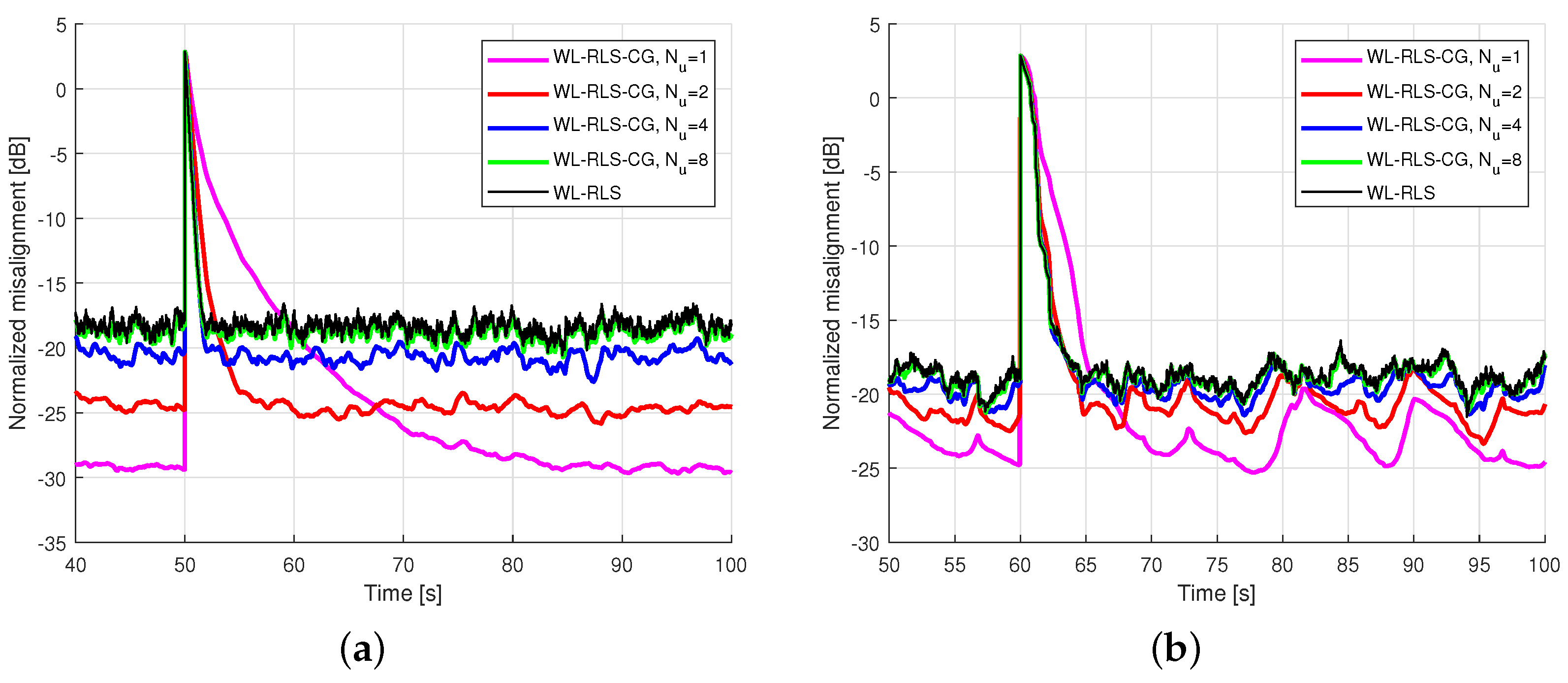
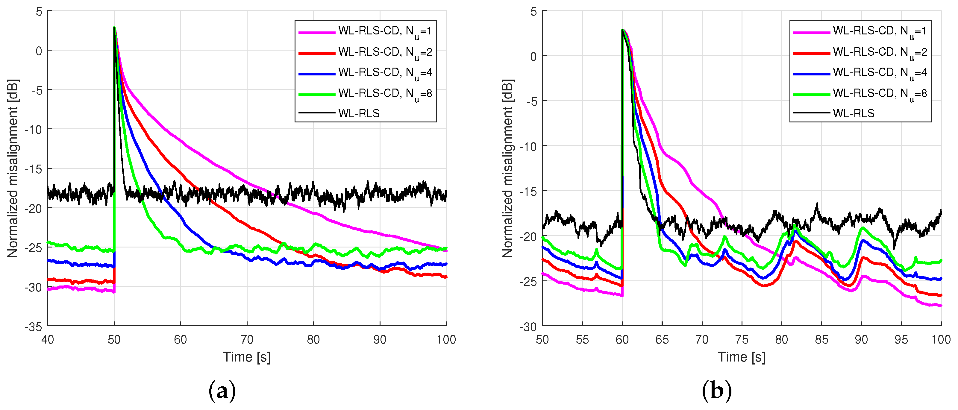
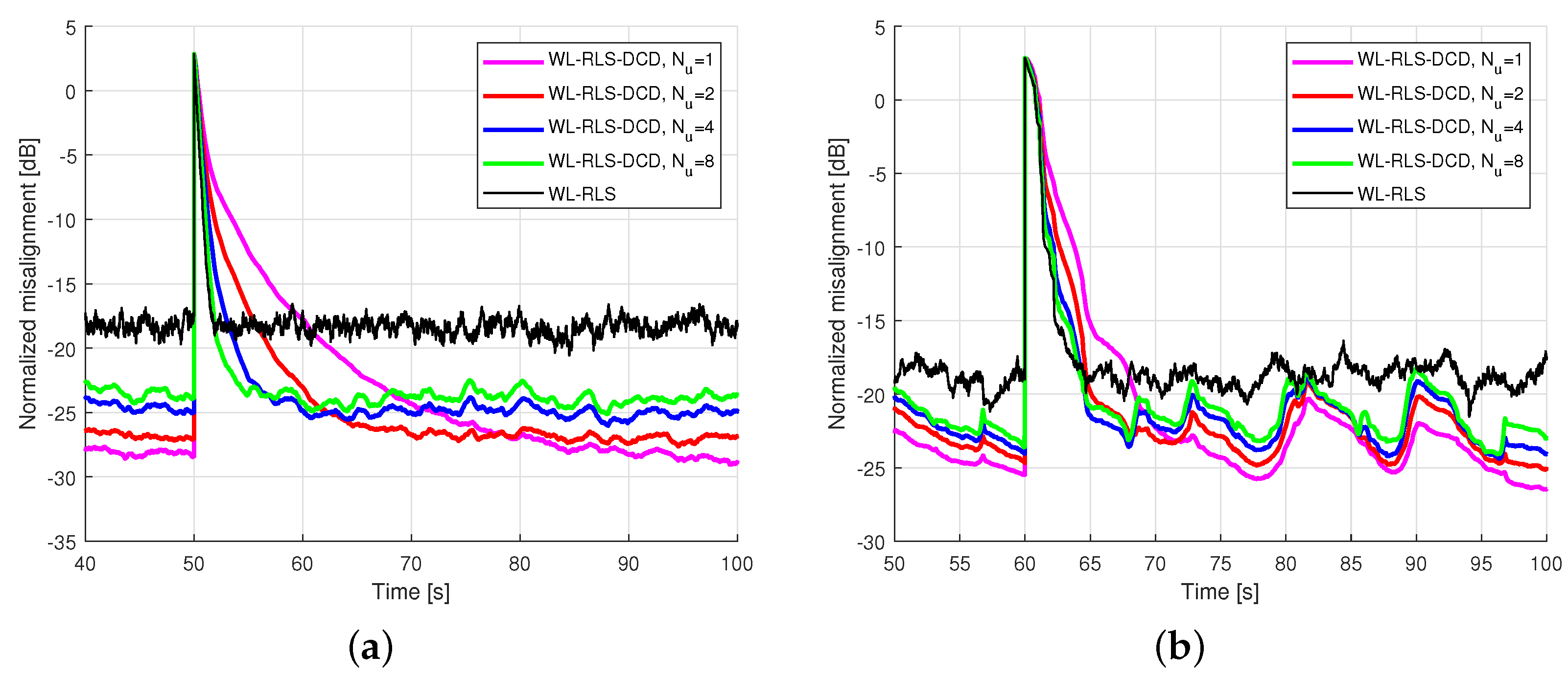
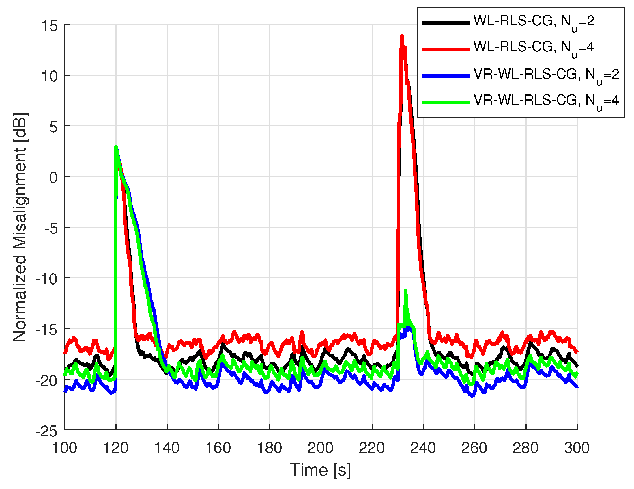
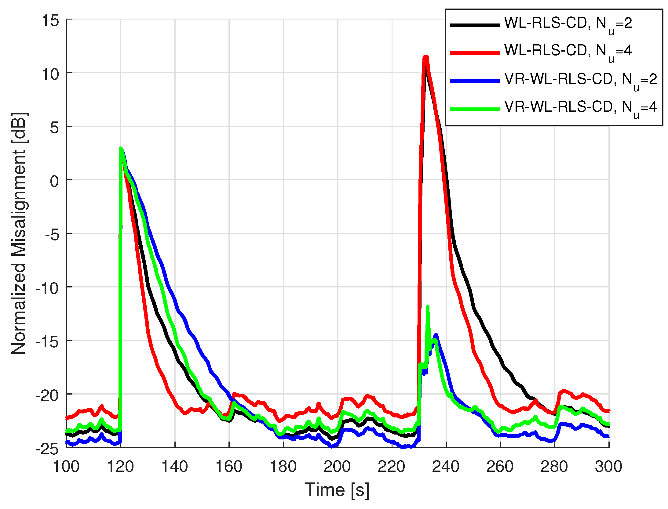
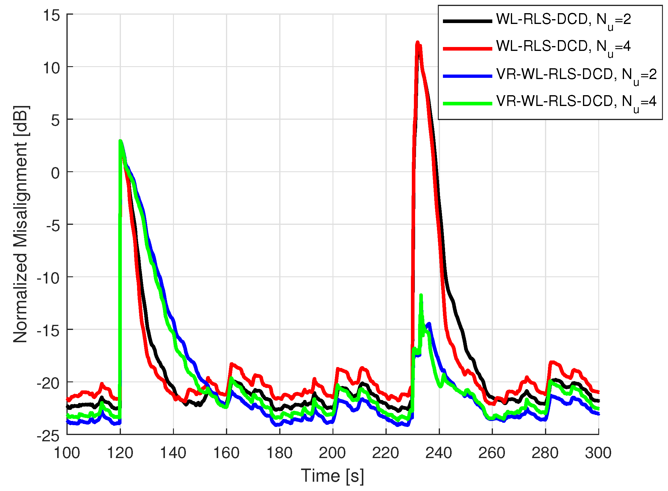
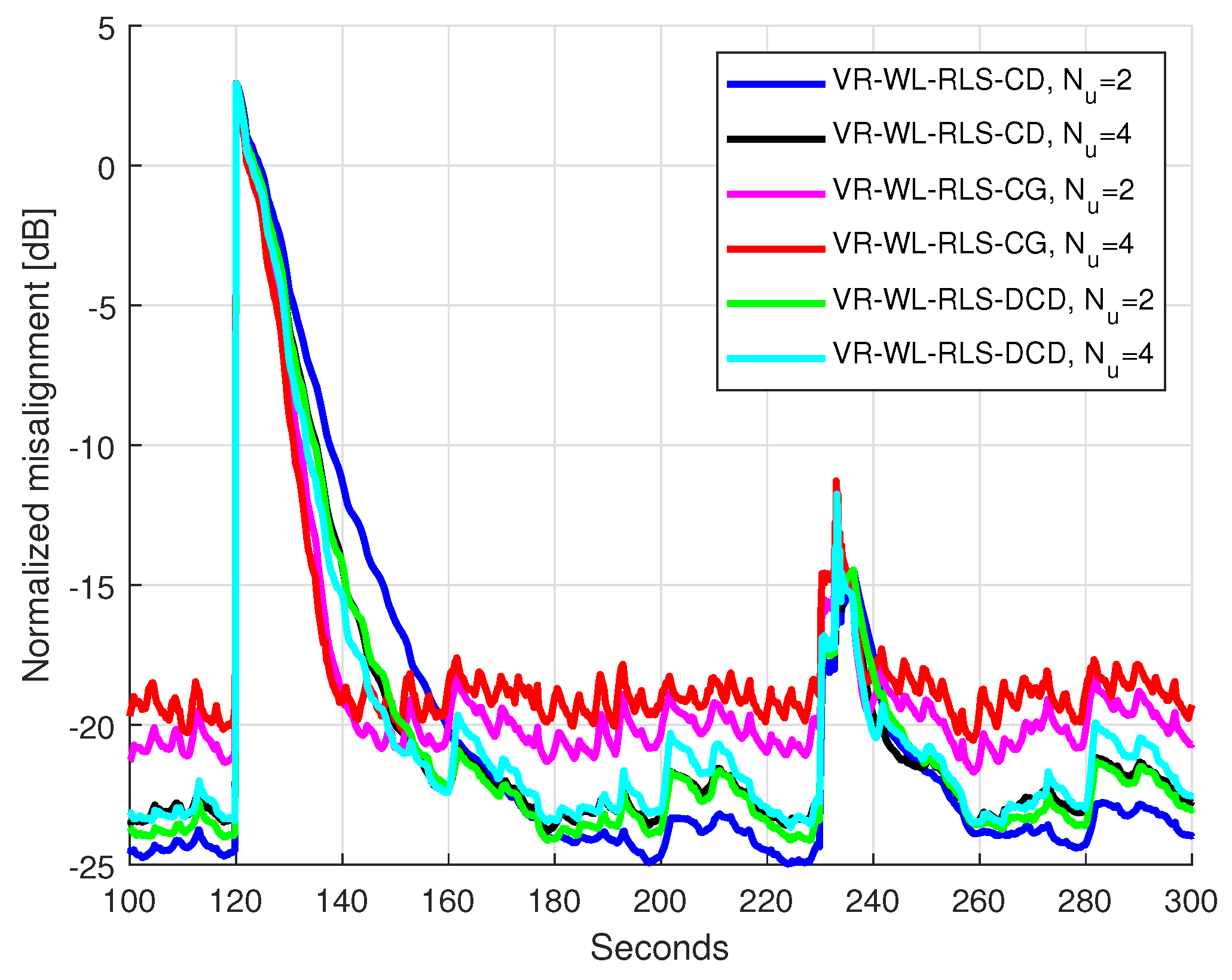
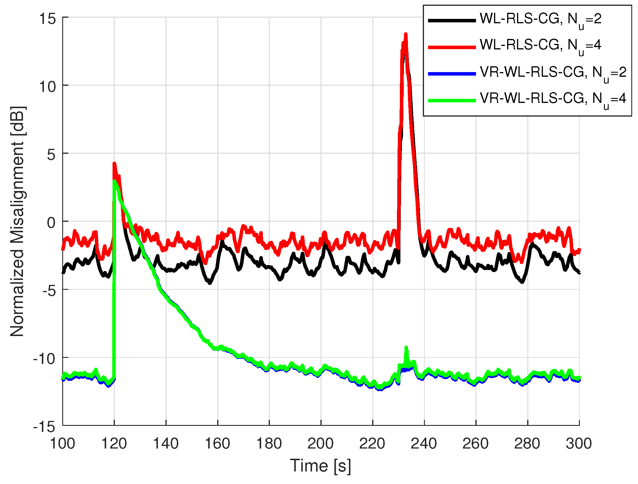
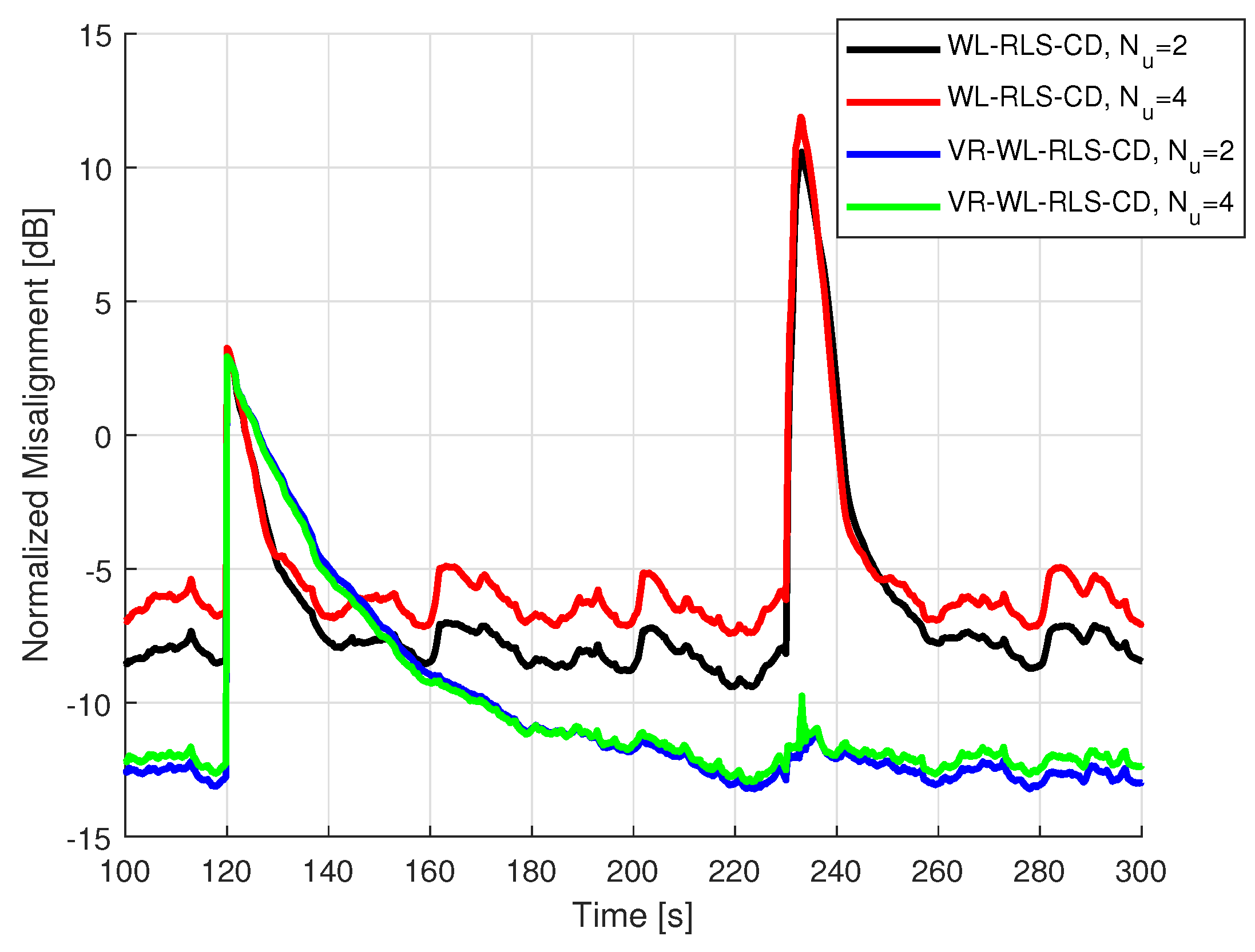
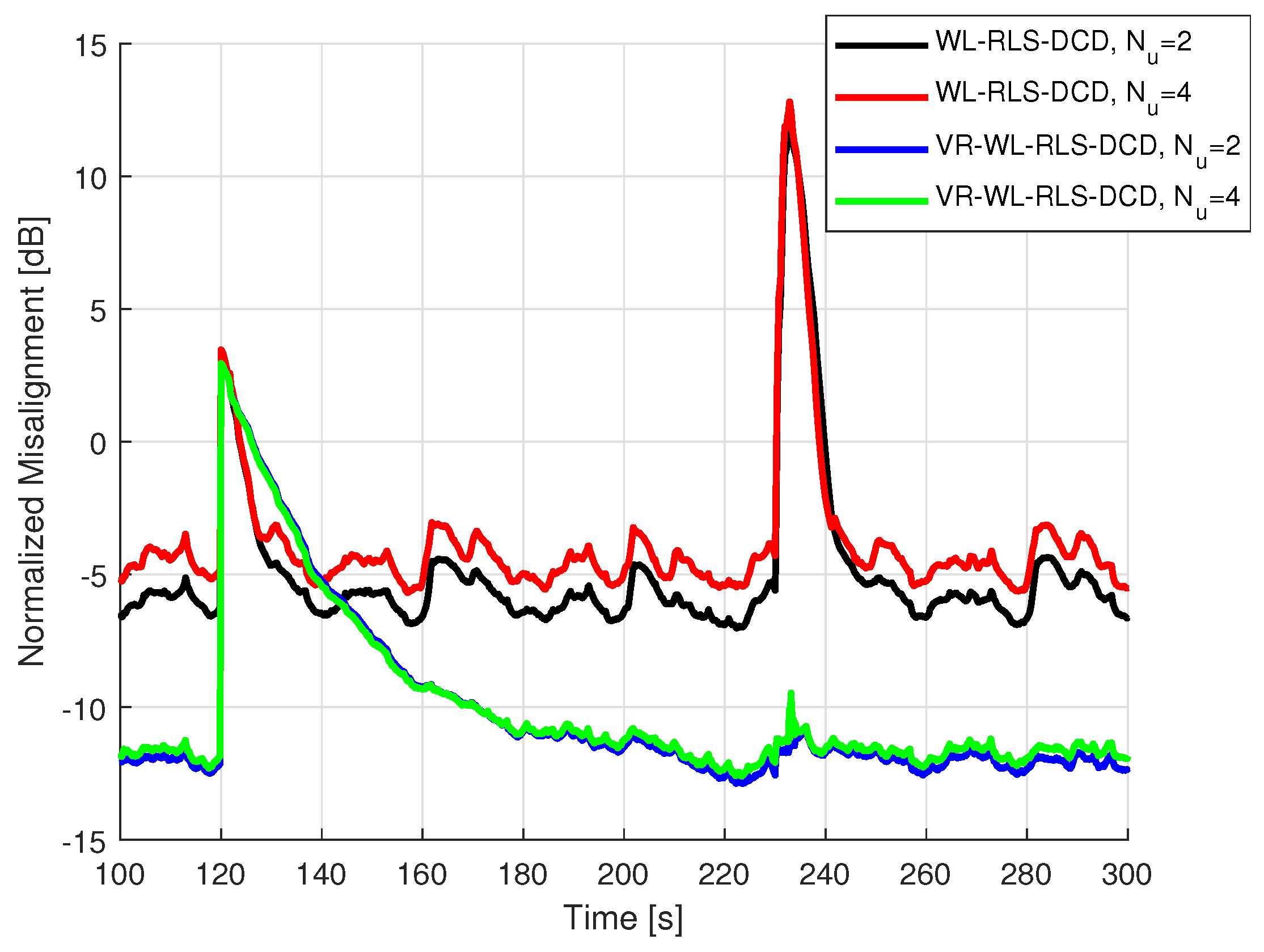
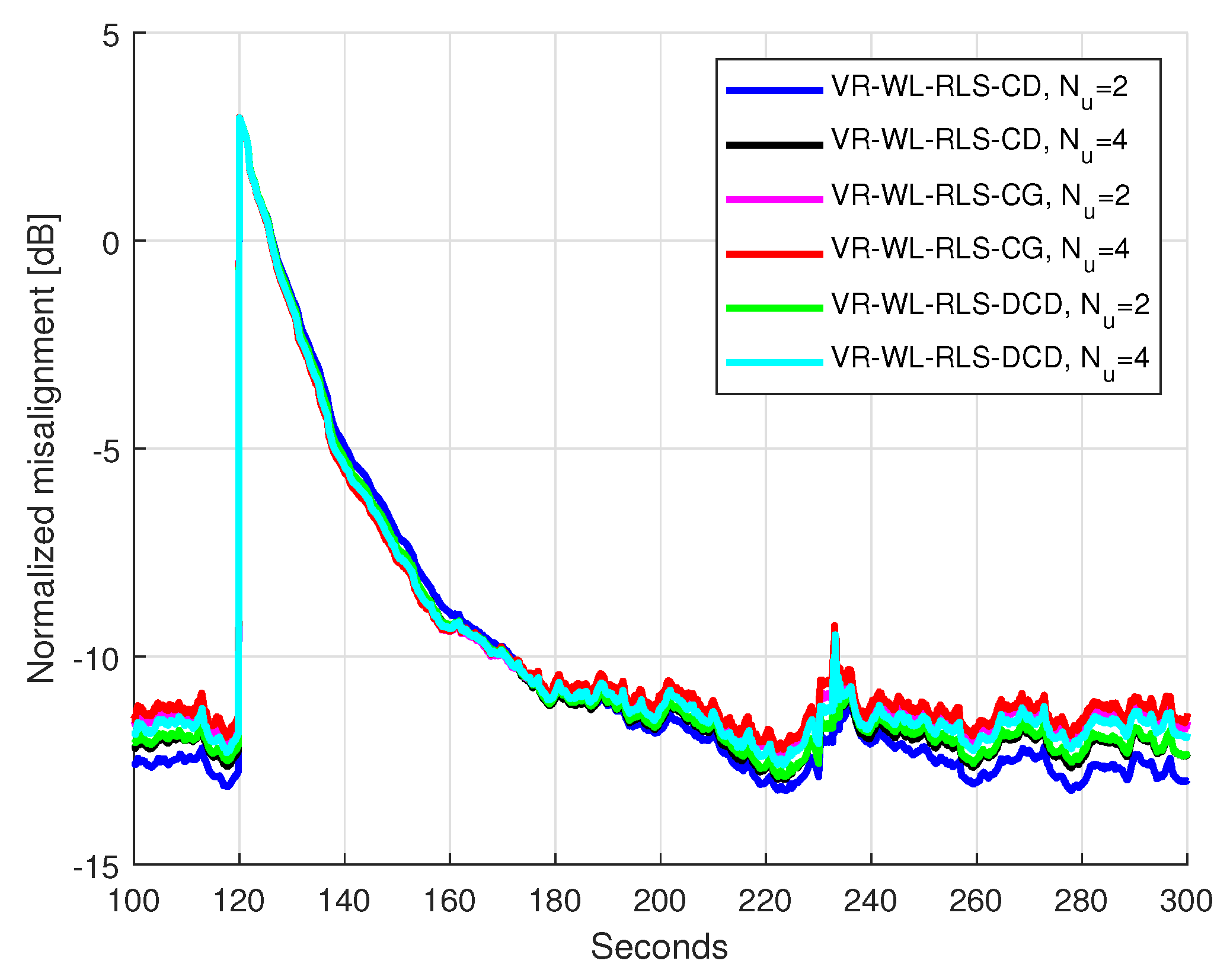
For the SAEC setup using different WL-RLS-LMS/VR-WL-RLS-LMS variants, we employed different types of input signals with different correlation properties, such as Gaussian noise sequences filtered through an autoregressive system with a single pole [AR(1)] with the value 0.99 or speech signals. Moreover, for each simulation, the original signal is filtered through two real-world acoustic paths in order to simulate the propagation from the acoustic source to each of the two microphones.

In comparison to single-channel acoustic echo cancellation (AEC) scenarios, the SAEC system has to mitigate the correlation between the two input channels, which can drastically reduce the performance of the adaptive algorithm. Therefore, after generating the two acoustic inputs, we use the predistortion block introduced in [6,11] in order to reduce the mentioned correlation. The samples of the new input signal can be expressed using the half-wave rectifier, as

$$\begin{array}{c}\hfill {\widehat{x}}_{{\mathrm{L}}_{\mathrm{c}}}\left(n\right)=x_{{\mathrm{L}}_{\mathrm{c}}}\left(n\right)+{\alpha }_{\mathrm{r}}\left[x_{{\mathrm{L}}_{\mathrm{c}}}\left(n\right)+\left|x_{{\mathrm{L}}_{\mathrm{c}}}\left(n\right)\right|\right]\end{array}$$

(46)

$$\begin{array}{c}\hfill {\widehat{x}}_{{\mathrm{R}}_{\mathrm{c}}}\left(n\right)=x_{{\mathrm{R}}_{\mathrm{c}}}\left(n\right)+{\alpha }_{\mathrm{r}}\left[x_{{\mathrm{R}}_{\mathrm{c}}}\left(n\right)-\left|x_{{\mathrm{R}}_{\mathrm{c}}}\left(n\right)\right|\right],\end{array}$$

(47)

where we can have the predistortion parameter ${\alpha }_{\mathrm{r}}<0.5$. In practice, the effect of ${\alpha }_{\mathrm{r}}$ is considered adequate for the interval $(0,0.25]$ in order to keep the distortion effect within acceptable limits. The new signals, ${\widehat{x}}_{{\mathrm{L}}_{\mathrm{c}}}\left(n\right)$ and ${\widehat{x}}_{{\mathrm{R}}_{\mathrm{c}}}\left(n\right)$, are computed before being reproduced by the loudspeakers and become the inputs of the complex-valued adaptive filter.

The four acoustic impulse responses generating the echo signals are also real-world measured impulse responses decimated to obtain the lengths $N=128$ and $N=256$. After combining them according to (8)–(10), the obtained complex echo path ${\mathbf{h}}_{\mathrm{t}}$ is employed at every filter iteration for measuring the normalized misalignment(NM) [6]:

$$\begin{array}{c}\hfill \mathrm{NM}\left(n\right)=10\lg {\displaystyle \frac{{∥{\mathbf{h}}_{\mathrm{t}}-\tilde{\mathbf{h}}\left(n\right)∥}_2^2}{{∥{\mathbf{h}}_{\mathrm{t}}∥}_2^2}}\left[\mathrm{dB}\right].\end{array}$$

(48)

Finally, when displaying simulation results using the performance criterion expressed in (48), we do not consider the initial convergence as relevant.

5.2. Results

For the first set of experiments, the WL-RLS-CG adaptive algorithm was studied in tracking scenarios with four acoustic echo paths having the length $N=128$. In order to simulate the acoustic echo impulse response changes, the corresponding sets of coefficients were shifted by 25 positions after some simulation time. For the input signals, we employed Gaussian noise filtered through the AR(1) system mentioned above with respect to a speech sequence.

The results are displayed in Figure 1a,b. The performance of the WL-RLS based on Woodbury’s identity was also added as a reference. It can be noticed that increasing the number of iterations $N_u$ leads to better tracking speeds, with the compromise of lower accuracy at a steady state. In Figure 1a, the WL-RLS-CG with the highest values of $N_u$ converge in less than 2 s and match the tracking speed of the WL-RLS. At steady state, the WL-RLS-CG with $N_u=4$ outperforms the WL-RLS by more than 5 dB for the NM value. The gap in performance between the different values of $N_u$ is narrower in Figure 1b, where the input is speech. As expected, the steady-state values for the NM are higher (i.e., lower accuracy with highly correlated input signals). The curves for $N_u\ge 2$, with respect to WL-RLS, have very similar tracking speeds, with only $N_u=2$ having consistent NM values below $-20$ dB at a steady state. Although for $N_u=1$ the NM approaches $-25$ dB for most of the time, its corresponding tracking speed is 2.5 seconds longer than the cases for $N_u\ge 2$ (i.e., double).

In both cases, above a certain value for the parameter $N_u$, the associated extra arithmetic workload does not provide satisfactory results (i.e., the tracking performances become capped for the higher values of $N_u$). The WL-RLS is the algorithm to match during the tracking period, and has the worst accuracy after convergence is achieved.

The scenarios discussed in the first set of experiments were repeated for the WL-RLS-CD adaptive algorithm (Figure 2a,b) with respect to the WL-RLS-DCD (Figure 3a,b). The differences between the tracking performances with respect to the value of the parameter $N_u$ are more evident in comparison to the WL-RLS-CG method. For the case of Figure 2a (the input is an AR(1) sequence), the WL-RLS has superior tracking speeds with respect to all versions of the WL-RLS-CD, including the variant with $N_u=8$, which requires two more seconds to reach a steady state after the echo paths change. In the scenario corresponding to speech input (i.e., for Figure 2b), the WL-RLS and the WL-RLS-CD with $N_u=8$ re-converge approximately at the same time. However, all the CD variants are more accurate at a steady state and attain NM values of less than $-25$ dB, while the WL-RLS rarely achieves misalignment values of $-20$ dB.

In Figure 3a,b, the WL-RLS-DCD benefit from the greedy nature of the DCD method and are able to match the tracking speeds of the WL-RLS algorithm for $N_u=4$, with respect to $N_u=8$. Similarly to the previous two figures, at a steady state, the WL-RLS-DCD outperforms the WL-RLS. The accuracy at steady state is better for both the WL-RLS-CD and the WL-RLS-DCD, with gaps of up to 9 dB for all values of $N_u$ in comparison to the reference WL-RLS.

For the following simulations, we consider that the tracking performances associated with all presented LSMs are suitable for $N_u>1$ and that a number of iterations, $N_u=8$, does not provide satisfactory improvements in performance in order to justify the corresponding arithmetic workload. Consequently, we will analyze the behavior of the different VR-WL-RLS-LSM versions for $N_u=2$ and $N_u=4$.

In Figure 4, the WL-RLS-CG and VR-WL-RLS-CG methods are studied when the acoustic echo paths change, and a DT situation occurs later in the same simulation. The tracking happens at the moment $t_0=120$ s, and the DT manifests in the interval $[230,234]$ seconds (i.e., another speech sequence is added to the microphone signals). The input signal is also speech. It can be noticed that the VR-WL-RLS-CG versions track the echo path changes approximately 10 s slower than the non-VR counterparts. However, they have better accuracy at steady state, and the VR-WL-RLS-CG with $N_u=2$ outperforms the VR variant with $N_u=4$.

When the DT situation occurs, the NM values associated with the WL-RLS-CG versions increase up to 14.5 dB. At the same time, both VR-WL-RLS-CG variants perform the update process in a slower manner, and the corresponding spikes in accuracy loss are situated at approximately $-11$ dB (more than 25 dB lower). Consequently, both VR variants return to the accuracy levels from before the DT occurrence with a delay of approximately 4 s (i.e., around a time of 238 s). Considering that the non-VR algorithms need more than 10 s to re-converge and attain previous accuracies at time 244 s, the results demonstrate that the accuracy penalties imposed on the VR-WL-RLS-CG filters are greatly diminished.

The same observations can be made when repeating the scenario for WL-RLS-CD and VR-WL-RLS-CD (Figure 5) with respect to WL-RLS-DCD and VR-WL-RLS-DCD (Figure 6). The VR versions suffer losses in terms of their tracking capabilities. Firstly, the WL-RLS-CD variants completely track the echo path changes approximately 10 s faster than their VR counterparts with the same $N_u$ values. However, when the DT occurs, the differences between accuracies are around 24 dB in favor of the VR-WL-RLS-CD variants.

Secondly, for the DCD-based algorithms, the differences in tracking capabilities are less influenced by the value of $N_u$ and more by employing the VR approach. Consequently, the VR-WL-RLS-DCD has similar tracking speeds for $N_u=2$ and $N_u=4$ and a 12–13 s delay for fully estimating the complex echo path after it changes (with respect to the WL-RLS-DCD). Nevertheless, in the DT interval, the non-VR algorithms have an NM of up to 13 dB, while the VR counterparts have accuracies no worse than $-12$ dB.

In Figure 7, all the VR versions from the three previous simulations are compared in the same scenario (i.e., first the tracking and then the DT period). It can be noticed that the VR-WL-RLS-CG has better convergence speeds, with a penalty in terms of accuracy at a steady state, with respect to the CD and the DCD versions. The VR-WL-RLS-DCD with both $N_u$ values and the VR-WL-RLS-CD with $N_u=4$ track the changes in the echo paths with a 5–6 s delay, and the VR-WL-RLS-CD with $N_u=2$ has the slowest reaction with a more than 15 s delay, with respect to the VR-WL-RLS-CG. However, at a steady state, the latter has NM values with minimum values of $-22$ dB, while the VR-WL-RLS-DCD and the VR-WL-RLS-CD with $N_u=4$ can easily reach $-23$ dB. The best steady-state results are obtained for VR-WL-RLS-CD for $N_u=2$ with NM values of around $-24$ and $-25$ dB. In the DT interval, all the methods have similar performances for both values of $N_u$ (the worst performance is situated around $-12$ dB). From a practical point of view, the VR-WL-RLS-CD and the VR-WL-RLS-DCD are more attractive because they require fewer arithmetic resources and deliver satisfactory results.

For the next experiments, the tracking and DT scenario was simulated again with the ENR set to 10 dB. In Figure 8 (WL-RLS-CG vs. VR-WL-RLS-CG), Figure 9 (WL-RLS-CD vs. VR-WL-RLS-CD), and Figure 10 (WL-RLS-DCD vs. VR-WL-RLS-DCD), it can be noticed that the difference in performance between the VR and non-VR algorithms has increased. At a steady state, all the algorithms have worse NM values with respect to the case of the scenarios with ENR = 25 dB. Although the delay in tracking manifests for all VR methods (like in previous cases), the performance reductions in the DT occurrences are smaller. The VR-WL-RLS-CG has a slight jump from $-11.5$ dB (at a steady state) to $-9.5$ for 3–4 s during the DT interval. Similarly, the VR-WL-RLS-CD has a performance reduction of $-2.5$ dB, and the VR-WL-RLS-DCD has a performance reduction of $-2$ dB, with the same re-convergence interval of less than 4 s. Moreover, we can notice that the discrepancies in performances between the VR and non-VR algorithms are higher than in the ENR = 25 dB scenarios. From the differences in 3–4 dB, the VR versions perform well and are more than 7 dB better in Figure 8, $-4.5$ dB in Figure 9, and $-6$ dB in Figure 10. The regularization leads to better accuracy at a steady state for all VR algorithms, and the update processes are almost unaffected by the DT occurrences.

Moreover, when only the VR versions are compared in Figure 11, the misalignment curves are very similar. Considering the compromise between performance and chip area costs, the VR-WL-RLS-DCD method can be considered the most attractive as the ENR decreases.

6. Conclusions

The paper describes and analyzes several RLS-LSM adaptive algorithms for SAEC applications. The WL framework employs complex-valued variables and simplifies the handling of the system. The exponentially weighted complex-valued RLS algorithm working within the WL model is combined with several LSMs in order to replace the classical system of equations with an auxiliary set of equations. Three types of LSMs are combined with the VR mechanism applied to the complex-valued RLS. The CG is the most costly method, which leads to an overall arithmetic complexity proportional to the square of the VR-WL-RLS-CG adaptive filter’s length. The CD and the DCD methods are progressively simpler in terms of arithmetic workloads and are designed to exploit the statistical properties of the input signals. Both VR-WL-RLS-CD and VR-WL-RLS-DCD require $\mathcal{O}\left(2N\right)$ multiplications, with an advantage for the latter, which solves the auxiliary system of equations using only additions and bit-shifts.

The simulation results demonstrate that the VR variants of WL-RLS-LMSs decrease the NM by approximately 25 dB during the DT intervals, with the compromise of reducing the tracking speeds of the corresponding algorithms. Moreover, the VR-WL-RLS-LMSs have better accuracy at a steady state with respect to the non-VR versions (at least 2–3 dB in terms of NM for ENR = 25 dB, and more than 7 dB in terms of NM for ENR = 10 dB). The performance gap at a steady state is better in favor of the VR variants as the ENR decreases.

The simulation results also showed that the greedy nature of the DCD iterations partially compensates for the tracking loss of VR-WL-RLS-DCD and allows it to match the tracking performances generated by VR-WL-RLS-CG. The associated robust performances in low-ENR conditions (including DT situations), combined with the overall arithmetic complexity (which is directly proportional to the adaptive filter’s length), make VR-WL-RLS-DCD an attractive candidate for hardware implementations for SAEC. Future research will concentrate on in-depth analysis for efficient hardware implementations (fixed-point vs. floating-point) of WL-RLS-DCD incorporating a VR approach.

References

1. Benesty, J.; Huang, Y. Adaptive Signal Processing–Applications to Real-World Problems; Springer: Berlin/Heidelberg, Germany, 2003. [Google Scholar]
2. Stanciu, C.; Benesty, J.; Paleologu, C.; Gänsler, T.; Ciochină, S. A widely linear model for stereophonic acoustic echo cancellation. Signal Process. 2013, 93, 511–516. [Google Scholar] [CrossRef]
3. Benesty, J.; Morgan, D.; Sondhi, M. A better understanding and an improved solution to the specific problems of stereophonic acoustic echo cancellation. IEEE Trans. Speech Audio Process. 1998, 6, 156–165. [Google Scholar] [CrossRef]
4. Diniz, P.S.R. Adaptive Filtering: Algorithms and Practical Implementation, 4th ed.; Springer: New York, NY, USA, 2013. [Google Scholar]
5. Sondhi, M.; Morgan, D.; Hall, J. Stereophonic acoustic echo cancellation-an overview of the fundamental problem. IEEE Signal Process. Lett. 1995, 2, 148–151. [Google Scholar] [CrossRef] [PubMed]
6. Benesty, J.; Paleologu, C.; Gänsler, T.; Ciochină, S. A Perspective on Stereophonic Acoustic Echo Cancellation; Springer: Berlin/Heidelberg, Germany, 2011; Volume 4. [Google Scholar] [CrossRef]
7. Hong, J. Stereophonic Acoustic Echo Suppression for Speech Interfaces for Intelligent TV Applications. IEEE Trans. Consum. Electron. 2018, 64, 153–161. [Google Scholar] [CrossRef]
8. Cho, B.J.; Park, H.M. Stereo Acoustic Echo Cancellation Based on Maximum Likelihood Estimation with Inter-Channel-Correlated Echo Compensation. IEEE Trans. Signal Process. 2020, 68, 5188–5203. [Google Scholar] [CrossRef]
9. Schneider, M.; Kellermann, W. Multichannel acoustic echo cancellation in the wave domain with increased robustness to nonuniqueness. IEEE/ACM Trans. Audio Speech Lang. Process. 2016, 24, 518–529. [Google Scholar] [CrossRef]
10. Lv, S.; Zhao, H.; Xu, W. Robust widely linear affine projection M-estimate adaptive algorithm: Performance analysis and application. IEEE Trans. Signal Process. 2023, 71, 3623–3636. [Google Scholar] [CrossRef]
11. Stanciu, C.; Benesty, J.; Paleologu, C.; Gänsler, T.; Ciochină, S. A novel perspective on stereophonic acoustic echo cancellation. In Proceedings of the IEEE International Conference on Acoustics, Speech and Signal Processing (ICASSP), Kyoto, Japan, 25–30 March 2012; pp. 25–28. [Google Scholar] [CrossRef]
12. Haykin, S. Adaptive Filter Theory; Prentice-Hall Information and System Sciences Series; Prentice Hall: Hoboken, NJ, USA, 2002. [Google Scholar]
13. Sayed, A. Adaptive Filters; Wiley: New York, NY, USA, 2008. [Google Scholar]
14. Chu, Y.J.; Chan, S.C. A New Local Polynomial Modeling-Based Variable Forgetting Factor RLS Algorithm and Its Acoustic Applications. IEEE/ACM Trans. Audio Speech Lang. Process. 2015, 23, 2059–2069. [Google Scholar] [CrossRef]
15. Romoli, L.; Cecchi, S.; Peretti, P.; Piazza, F. A Mixed Decorrelation Approach for Stereo Acoustic Echo Cancellation Based on the Estimation of the Fundamental Frequency. IEEE Trans. Audio Speech Lang. Process. 2012, 20, 690–698. [Google Scholar] [CrossRef]
16. Romoli, L.; Cecchi, S.; Piazza, F. A novel decorrelation approach for multichannel system identification. In Proceedings of the 2014 IEEE International Conference on Acoustics, Speech and Signal Processing (ICASSP), Florence, Italy, 4–9 May 2014; pp. 6652–6656. [Google Scholar] [CrossRef]
17. Paleologu, C.; Benesty, J.; Ciochină, S. Data-Reuse Recursive Least-Squares Algorithms. IEEE Signal Process. Lett. 2022, 29, 752–756. [Google Scholar] [CrossRef]
18. Hänsler, E.; Schmidt, G. Acoustic Echo and Noise Control—A Practical Approach; Wiley: Hoboken, NJ, USA, 2004. [Google Scholar]
19. Zakharov, Y.V.; White, G.P.; Liu, J. Low-Complexity RLS Algorithms Using Dichotomous Coordinate Descent Iterations. IEEE Trans. Signal Process. 2008, 56, 3150–3161. [Google Scholar] [CrossRef]
20. Liu, J.; Zakharov, Y.V.; Weaver, B. Architecture and FPGA Design of Dichotomous Coordinate Descent Algorithms. IEEE Trans. Circuits Syst. I Regul. Pap. 2009, 56, 2425–2438. [Google Scholar] [CrossRef]
21. Zakharov, Y.V.; Nascimento, V.H. DCD-RLS Adaptive Filters With Penalties for Sparse Identification. IEEE Trans. Signal Process. 2013, 61, 3198–3213. [Google Scholar] [CrossRef]
22. Yu, Y.; Lu, L.; Zheng, Z.; Wang, W.; Zakharov, Y.; de Lamare, R.C. DCD-Based Recursive Adaptive Algorithms Robust Against Impulsive Noise. IEEE Trans. Circuits Syst. II Express Briefs 2020, 67, 1359–1363. [Google Scholar] [CrossRef]
23. Paleologu, C.; Benesty, J.; Ciochină, S. A Robust Variable Forgetting Factor Recursive Least-Squares Algorithm for System Identification. IEEE Signal Process. Lett. 2008, 15, 597–600. [Google Scholar] [CrossRef]
24. Malik, S.; Wung, J.; Atkins, J.; Naik, D. Double-Talk Robust Multichannel Acoustic Echo Cancellation Using Least-Squares MIMO Adaptive Filtering: Transversal, Array, and Lattice Forms. IEEE Trans. Signal Process. 2020, 68, 4887–4902. [Google Scholar] [CrossRef]
25. Zhang, Y.; Wu, T.; Zakharov, Y.V.; Li, J. MMP-DCD-CV based sparse channel estimation algorithm for underwater acoustic transform domain communication system. Appl. Acoust. 2019, 154, 43–52. [Google Scholar] [CrossRef]
26. Liao, M.; Zakharov, Y.V. DCD-based joint sparse channel estimation for OFDM in virtual angular domain. IEEE Access 2021, 9, 102081–102090. [Google Scholar] [CrossRef]
27. Yu, Y.; Lu, L.; Zakharov, Y.; de Lamare, R.C.; Chen, B. Robust sparsity-aware RLS algorithms with jointly-optimized parameters against impulsive noise. IEEE Signal Process. Lett. 2022, 29, 1037–1041. [Google Scholar] [CrossRef]
28. Yu, Y.; Huang, Z.; He, H.; Zakharov, Y.; de Lamare, R.C. Sparsity-aware robust normalized subband adaptive filtering algorithms with alternating optimization of parameters. IEEE Trans. Circuits Syst. II Express Briefs 2022, 69, 3934–3938. [Google Scholar] [CrossRef]
29. Niedźwiecki, M.; Gańcza, A.; Shen, L.; Zakharov, Y. Adaptive identification of sparse underwater acoustic channels with a mix of static and time-varying parameters. Signal Process. 2022, 200, 108664. [Google Scholar] [CrossRef]
30. Yu, Y.; Ye, J.; Zakharov, Y.; He, H. Robust proportionate subband adaptive filter algorithms with optimal variable step-size. IEEE Trans. Circuits Syst. II Express Briefs 2024, in press. [CrossRef]
31. Benesty, J.; Paleologu, C.; Ciochina, S. Regularization of the RLS Algorithm. IEICE Trans. Fundam. Electron. Commun. Comput. Sci. 2011, E94.A, 1628–1629. [Google Scholar] [CrossRef]
32. Elisei-Iliescu, C.; Stanciu, C.L.; Paleologu, C.; Benesty, J.; Anghel, C.; Ciochină, S. Robust Variable-Regularized RLS Algotihms. In Proceedings of the 2017 Hands-Free Speech Communications and Microphone Arrays (HSCMA), San Francisco, CA, USA, 1–3 March 2017. [Google Scholar] [CrossRef]
33. Stanciu, C.; Anghel, C.; Stanciu, L. Efficient FPGA implementation of the DCD-RLS algorithm for stereo acoustic echo cancellation. In Proceedings of the 2015 International Symposium on Signals, Circuits and Systems (ISSCS), Iasi, Romania, 9–10 July 2015; pp. 1–4. [Google Scholar] [CrossRef]
34. Elisei-Iliescu, C.; Paleologu, C.; Benesty, J.; Stanciu, C.; Anghel, C.; Ciochină, S. Recursive Least-Squares Algorithms for the Identification of Low-Rank Systems. IEEE/ACM Trans. Audio Speech Lang. Process. 2019, 27, 903–918. [Google Scholar] [CrossRef]
35. Chang, P.S.; Willson, A.N. Analysis of Conjugate Gradient Algorithms for Adaptive Filtering. IEEE Trans. Signal Process. 2000, 48, 409–418. [Google Scholar] [CrossRef]
Figure 1. Misalignment of the WL-RLS and WL-RLS-CG for different values of N u . The input signal is an AR(1) sequence with the pole 0.99 for (a), with respect to a speech sequence for (b). The input signals are predistorted with α r = 0.175 . The length of the four unknown impulse responses is N = 128 and λ = 1 1 / ( 16 N ) . The echo paths change at time index t a = 50 s for scenario (a), with respect to t b = 60 s. The ENR is experimentally set to 25 dB.
Electronics 13 01479 g001
Figure 2. Misalignment of the WL-RLS and WL-RLS-CD for different values of N u . The input signal is an AR(1) sequence with the pole 0.99 for (a), with respect to a speech sequence for (b). The input signals are predistorted with α r = 0.175 . The length of the four unknown impulse responses is N = 128 and λ = 1 1 / ( 16 N ) . The echo paths change at time index t a = 50 s for scenario (a), with respect to t b = 60 s. The ENR is experimentally set to 25 dB.
Electronics 13 01479 g002
Figure 3. Misalignment of WL-RLS and WL-RLS-DCD for different values of N u . The input signal is an AR(1) sequence with the pole 0.99 for (a), with respect to a speech sequence for (b). The input signals are predistorted with α r = 0.175 . The length of the four unknown impulse responses is N = 128 and λ = 1 1 / ( 16 N ) . The echo paths change at time index t a = 50 s for scenario (a), with respect to t b = 60 s. The ENR is experimentally set to 25 dB.
Electronics 13 01479 g003
Figure 4. Misalignment of WL-RLS-CG and VR-WL-RLS-CG for different values of N u . The input signal is a speech sequence. Input signals are predistorted with α r = 0.175 . The length of the four unknown impulse responses is N = 256 , λ = 1 1 / ( 64 N ) , and for the VR algorithm, it is γ = 0.999 . The echo paths change at time index t 0 = 120 , and a DT situation occurs in the time interval [230, 234] s. The ENR is experimentally set to 25 dB.
Electronics 13 01479 g004
Figure 5. Misalignment of WL-RLS-CD and VR-WL-RLS-CD for different values of N u . The input signal is a speech sequence. Input signals are predistorted with α r = 0.175 . The length of the four unknown impulse responses is N = 256 , λ = 1 1 / ( 64 N ) , and for the VR algorithm, it is γ = 0.999 . The echo paths change at time index t 0 = 120 , and a DT situation occurs in the time interval [230, 234] s. The ENR is experimentally set to 25 dB.
Electronics 13 01479 g005
Figure 6. Misalignment of the WL-RLS-DCD and VR-WL-RLS-DCD for different values of N u . The input signal is a speech sequence. Input signals are predistorted with α r = 0.175 . The length of the four unknown impulse responses is N = 256 and λ = 1 1 / ( 64 N ) , and for the VR algorithm, it is γ = 0.999 . The echo paths change at time index t 0 = 120 , and a DT situation occurs in the time interval [230, 234] s. The ENR is experimentally set to 25 dB.
Electronics 13 01479 g006
Figure 7. Misalignment of the VR-WL-RLS-CG, VR-WL-RLS-CD, and VR-WL-RLS-DCD for different values of N u . The input signal is a speech sequence. The input signals are predistorted with α r = 0.175 . The length of the four unknown impulse responses is N = 256 , λ = 1 1 / ( 64 N ) , and γ = 0.999 . The echo paths change at time index t 0 = 120 , and a DT situation occurs in the time interval [230, 234] s. The ENR is experimentally set to 25 dB.
Electronics 13 01479 g007
Figure 8. Misalignment of WL-RLS-CG and VR-WL-RLS-CG for different values of N u . The input signal is a speech sequence. The input signals are predistorted with α r = 0.175 . The length of the four unknown impulse responses is N = 256 , λ = 1 1 / ( 64 N ) , and for the VR algorithm, it is γ = 0.999 . The echo paths change at time index t 0 = 120 , and a DT situation occurs in the time interval [230, 234] s. The ENR is experimentally set to 10 dB.
Electronics 13 01479 g008
Figure 9. Misalignment of the WL-RLS-CD and VR-WL-RLS-CD for different values of N u . The input signal is a speech sequence. Input signals are predistorted with α r = 0.175 . The length of the four unknown impulse responses is N = 256 , λ = 1 1 / ( 64 N ) , and for the VR algorithm γ = 0.999 . The echo paths change at time index t 0 = 120 , and a DT situation occurs in the time interval [230, 234] s. The ENR is experimentally set to 10 dB.
Electronics 13 01479 g009
Figure 10. Misalignment of WL-RLS-DCD and VR-WL-RLS-DCD for different values of N u . The input signal is a speech sequence. Input signals are predistorted with α r = 0.175 . The length of the four unknown impulse responses is N = 256 , λ = 1 1 / ( 64 N ) , and for the VR algorithm, it is γ = 0.999 . The echo paths change at time index t 0 = 120 , and a DT situation occurs in the time interval [230, 234] s. The ENR is experimentally set to 10 dB.
Electronics 13 01479 g010
Figure 11. Misalignment of VR-WL-RLS-CG, VR-WL-RLS-CD, and VR-WL-RLS-DCD for different values of N u . The input signal is a speech sequence. The input signals are predistorted with α r = 0.175 . The length of the four unknown impulse responses is N = 256 , λ = 1 1 / ( 64 N ) , and γ = 0.999 . The echo paths change at time index t 0 = 120 , and a DT situation occurs in the time interval [230, 234] s. The ENR is experimentally set to 10 dB.
Electronics 13 01479 g011