Nonrelativistic Quantum Mechanical Problem for the Cornell Potential in Lobachevsky Space

Abstract

In Friedmann–Lobachevsky space-time with a radius of curvature slowly varying over time, we study numerically the problem of motion of a particle moving in the Cornell potential. The mass of the particle is taken to be a reduced mass of the charmonium system. In contrast to the similar problem in flat space, in Lobachevsky space the Cornell potential has a finite depth and, as a consequence, the number of bound states of the system is finite and motion with a continuum energy spectrum is also possible. In this paper, we study the bound states as well as the scattering states of the system.

1. Introduction

The centennial anniversary of the publication of the seminal paper by A.A. Friedmann [1], followed by related publications [2,3,4], motivated the present discussion on the role of geometrical ideas in particle physics and cosmology.

During 1922–1924, A. Friedmann derived his celebrated dynamical equations for the universe. Many details from Friedmann’s biography can be found in the book [5]. He started from the General Relativity equations with arbitrary cosmological “constant” and opened the way to building models of a non-stationary universe. The non-stationary nature of the universe was brilliantly confirmed in astronomical observations by Hubble. Following Friedmann, a large number of models of the expanding universe were suggested (see, e.g., [6,7,8]).

In the beginning of the quark hypothesis of particle structure, composite models based on non-relativistic problems for various potentials demonstrated their effectiveness. Within the framework of that approach, the mass spectra of a number of mesons and hadrons and some of their static characteristics were successfully described. Examples of the use of such models are given in reviews [9,10,11]. In approaches in which particles are considered as consisting of quarks, a special role belongs to the Cornell potential, which ensures confinement of quarks (see, for example, [12]). As far as we know, the quantum-mechanical problem of a particle moving in the Cornell potential in Lobachevsky space has not yet been discussed in the literature, although coupled systems like the b-meson have been studied in a number of papers [13,14].

Now, more than 100 years after the creation of General Relativity, we may ask ourselves: what is its most unexpected and surprising prediction? There is no doubt that the answer should be the theory of an expanding universe, created by Alexander Friedmann [1,2,3]. This was also a triumph of non-Euclidean geometry, as proposed by J. Bolyai, C. F. Gauss, N. I. Lobachevsky (BGL), developed by Bernhard Riemann, and extended by Hermann Minkowski in a space-time manifold.

About 30 years later, George Gamow wrote in his book [15] “The Creation of the Universe”:

…the Russian mathematician A. Friedmann pointed out that the static nature of Einstein’s universe was the result of an algebraic mistake (essentially a division by zero) made in the process of its derivation. Friedmann then went on to show that the correct treatment of Einstein’s basic equations leads to a class of expanding and contracting universes…

In 1965, Erast B. Gliner [16] assumed that the pressure in Einstein–Friedmann equations for the very early universe is proportional to the energy density with a negative sign. This unusual relation between pressure and energy density was the first theoretical prediction of dark energy, now confirmed by observations. In subsequent papers [17,18], he found an exponentially increasing solution of these equations contributing to the development of cosmology with a rapid expansion phase, followed by a large number of inflationary cosmological models.

Simultaneously and independently of Gliner, a related activity preceding numerous papers on inflation took place in Kiev. The common feature in these papers was the exponential expansion of the universe, now called inflation, provided by negative pressure in the equation of state $p\left(T\right)$.

The relevant derivation is simple. In Fridmann’s homogeneous, isotropic and flat universe the scale factor $\rho$ obeys the equations

$$\begin{array}{c}\hfill \dot{\rho }-G\rho \sqrt{ϵ}=0,\end{array}$$

(1)

$$\begin{array}{c}\hfill \dot{ϵ}+3\dot{\rho }/\rho (ϵ+p)=0,\end{array}$$

(2)

where p is pressure and $G=\sqrt{8\pi /3}/M_p$. From Equations (1) and (2),

$$\ddot{\rho }=-G^2\rho (ϵ+3p)/2$$

(3)

follows, whence $3p+ϵ<0$ for inflationary solutions. As energy density is positive, the above inequality produces inflation only at negative pressure [19].

Historically, this was predicted in [7] from an equation of state of strongly interacting (nuclear) matter derived [7] in the framework of the S matrix formulation of statistical mechanics. It is interesting by itself and may have interesting consequences in nuclear and particle physics. Inflation resulting from this minimum was a bonus [19].

Here, several comments are in order. First, the rate of this kind of inflation is modest with respect to the popular scenarios. For this reason, it was also called [20,21] “tepid” compared to the alternative violent expansion. Furthermore, it may have occurred later with respect to those based on the Standard Theory. One cannot exclude a sequence of inflations of the early universe. The above “nuclear” one was the latest in time and it may have washed away the footprints of the earlier ones.

2. Quark–Antiquark Bound States in Lobachevsky Space

Einstein’s famous work [22], in which he introduced the cosmological constant and obtained the first cosmological solution, was the impetus for further research in the theory of relativity, quantum mechanics and theory for non-relativistic particles moving in curved spaces [23,24,25,26,27,28,29,30].

We will consider Friedmann-Lobachevsky space-time based on the assumption that the curvature radius $\rho \left(t\right)$ changes very slowly in time, and is considered as being constant, in particular, as it is in Einstein’s solution [22]. Taking into account the uncertainty of the right side of Equation (3), we accept the assumption for a period of time $\delta t$ satisfying the inequality ${\rho }^{\prime }\left(t_0\right)\delta t\ll \rho \left(t_0\right)$ or $\delta t\ll H^{-1}$, where H is Hubble constant [31].

The Schrödinger equation for stationary states in Lobachevsky space with curvature radius $\rho$ in spherical coordinates,

$$x_0=\rho cosh\beta ;x_1=\rho sinh\beta sin\theta cos\varphi ;$$

$$x_2=\rho sinh\beta sin\theta sin\varphi ;x_3=\rho sinh\beta cos\theta ;$$

$$0\le \beta <\infty ;0\le \theta \le \pi ;0\le \varphi \le 2\pi ,$$

(4)

has the form

$$-\frac{\hslash }{2m}\left(\frac{1}{{\rho }^2{sinh}^2\beta }\frac{\partial }{\partial \beta }\left({sinh}^2\beta \frac{\partial }{\partial \beta }\right)+\frac{1}{{\rho }^2{sinh}^2\beta }{\Delta }_{\theta ,\varphi }\right)\psi +V\psi =E\psi ,$$

(5)

where $\beta =r/\rho$.

Here, we use the embedding of Lobachevsky space into a four-dimensional pseudo-Euclidean space, in which the rectangular coordinates $x_{\mu }$, $\mu =1,2,3,4$ are introduced, and for points in Lobachevsky space the equality

$$x_{\mu }{x}_{\mu }={\mathbf{x}}^2+x_4^2={\mathbf{x}}^2-x_0^2=-{\rho }^2,\mathbf{x}=(x_1,x_2,x_3),x_4=i{x}_0$$

(6)

is valid.

In the case of a central symmetric potential $V=V\left(r\right)$, Equation (5) can be reduced to

$$-\frac{1}{2}\frac{d^{2}u}{d{r}^2}+V_{eff}\left(r\right)u=ϵu,$$

(7)

where the effective potential is

$$V_{eff}\left(r\right)=mV\left(r\right)+\frac{l(l+1)}{2{\rho }^2{sinh}^2(r/\rho )}+\frac{1}{2{\rho }^2},$$

(8)

and $ϵ=mE$.

In this case, the wavefunction is written in terms of $u\left(r\right)$ and the spherical harmonics as

$$\psi (r,\theta ,\varphi )=\frac{u\left(r\right)}{sinh(r/\rho )}{Y}_{lm}(\theta ,\varphi ).$$

(9)

Here, a rational system of units has been chosen, in which $c=\hslash =1$ and all physical quantities have units of measurement of powers of mass—namely, ${\left(GeV\right)}^a$, wherein $\left[r\right]=\left[\rho \right]=Ge{V}^{-1}$, $\left[m\right]=GeV$, $\left[V\right(r\left)\right]=\left[E\right]=GeV$, $\left[ϵ\right]=\left[V_{eff}\right]=Ge{V}^2$.

Let us consider the motion of a particle whose mass is equal to the reduced mass of two c quarks (a system of a c quark and its anti-quark is called charmonium)—that is, let us take $m=0.635GeV$. Assume that such a particle moves in a field in which its potential energy is described by the Cornell potential, the expression for which in Lobachevsky space has the form

$$V\left(r\right)=\frac{a}{\rho }coth\frac{r}{\rho }+b\rho \tanh \frac{r}{\rho }.$$

(10)

Note that the choice of the Cornell potential is generally ambiguous. We proceeded from the fact that the first term is a fundamental solution of the Laplace–Beltrami equation in three-dimensional Lobachevsky space, and we sought to preserve the symmetry inherent in the flat limit of this potential. In Formula (10), the first term corresponds to the Coulomb attraction and the second to the linearly increasing potential in flat space.

For parameters a and b we take the following values [11]:

$$a=-0.52;b=0.18Ge{V}^2.$$

In Lobachevsky space, the depth of the well of the effective potential is finite and it depends on the orbital quantum number l and the radius of curvature $\rho$. As l increases (keeping $\rho$ constant) the well becomes more and more shallow, and at some high-enough value of l it disappears: no bound states are possible. On the contrary, as we increase $\rho$ and keep l unchanged, the well becomes deeper and we can have more bound states. In the limit when $\rho ⟶\infty$ we are back to the flat space with an infinite number of bound states. The Cornell potential formula in Lobachevsky space also leads to that of the flat space in this limit. When $\rho$ is small enough (which corresponds to the high curvature of the space, as it is supposed to take place in the early universe) the well again disappears and we do not have bound states. As the curvature radius increases in time (Friedmann’s solution for the open-universe model) a particle moving in the Cornell potential at first has no bound states; then, it has a larger and larger finite number of bound states and, as $\rho$ approaches infinity (flat space), all states become bound.

When $r⟶0$ the asymptotic behavior of the solution to Equation (7) is

$$u\sim {\left(\tanh (r/\rho )\right)}^{l+1}.$$

(11)

Indeed, at $r⟶0$ centrifugal energy makes the greatest contribution to the equation and the approximate equation has the form

$$-\frac{d^{2}u}{d{\beta }^2}+\frac{l(l+1)}{{sinh}^2\left(\beta \right)}u=0.$$

The last equation has the following solution that is regular at zero:

$$u={{\left(\tanh \beta \right)}^{l+1}}_2{F}_1\left(1+\frac{l}{2},\frac{1}{2}+\frac{l}{2},\frac{3}{2}+l,{\tanh }^2\beta \right)\approx {\left(\tanh \beta \right)}^{l+1}.$$

We will study Equation (7) using numerical methods: namely, we will find the energies of bound states. To do so, we apply the shooting method, at each step of which the differential Equation (7) is numerically solved under initial conditions specified by the asymptotic expressions

$$u\left(r_0\right)={\left[\tanh (r_0/\rho )\right]}^{l+1};u^{\prime }\left(r_0\right)=\frac{(l+1){\left[\tanh (r_0/\rho )\right]}^l}{\rho {cosh}^2(r_0/\rho )},$$

(12)

where $r_0=0.001Ge{V}^{-1}$—variable value close to zero.

Figure 1 shows a plot of the effective interaction potential at $\rho =8Ge{V}^{-1}$, $l=1$.

It can be seen that in Lobachevsky space the effective interaction potential has the form of a potential well of finite depth, whereas in flat space for the Cornell potential we have an infinitely deep potential well. Let us denote

$${ϵ}_{max}=\underset{r\to \infty }{lim}{V}_{eff}\left(r\right)=m\left(\frac{a}{\rho }+b\rho \right)+\frac{1}{2{\rho }^2}.$$

(13)

While scattering prevails at energies higher than ${ϵ}_{max}/m$, bound states are possible at lower energies.

Figure 2 shows numerical solutions for bound states and their corresponding energy levels for $\rho =8Ge{V}^{-1}$, $l=1$. In this case, there are only four bound states.

As the depth of the well increases with increasing $\rho$ and decreases with increasing l, we can expect that the number of bound states will be greater for the larger values of $\rho$ and the smaller values of l. Figure 3 shows the results of the numerical calculation of the number of bound states for different values of $\rho$ and l.

Using the numerically calculated values of energy levels at different l, Regge trajectories are constructed at $\rho =10Ge{V}^{-1}$ (see Figure 4). Here, we use the same approach as in [32,33]. It can be seen from the figure that as l increases the number of bound states decreases.

It should be noted that the above Regge trajectories differ from those resulting from analyticity and duality [34]. While the above are convex up and infinitely rising, those based on analyticity, unitarity and duality are concave down, with limited real parts, predicting a finite number of resonances (see [34]).

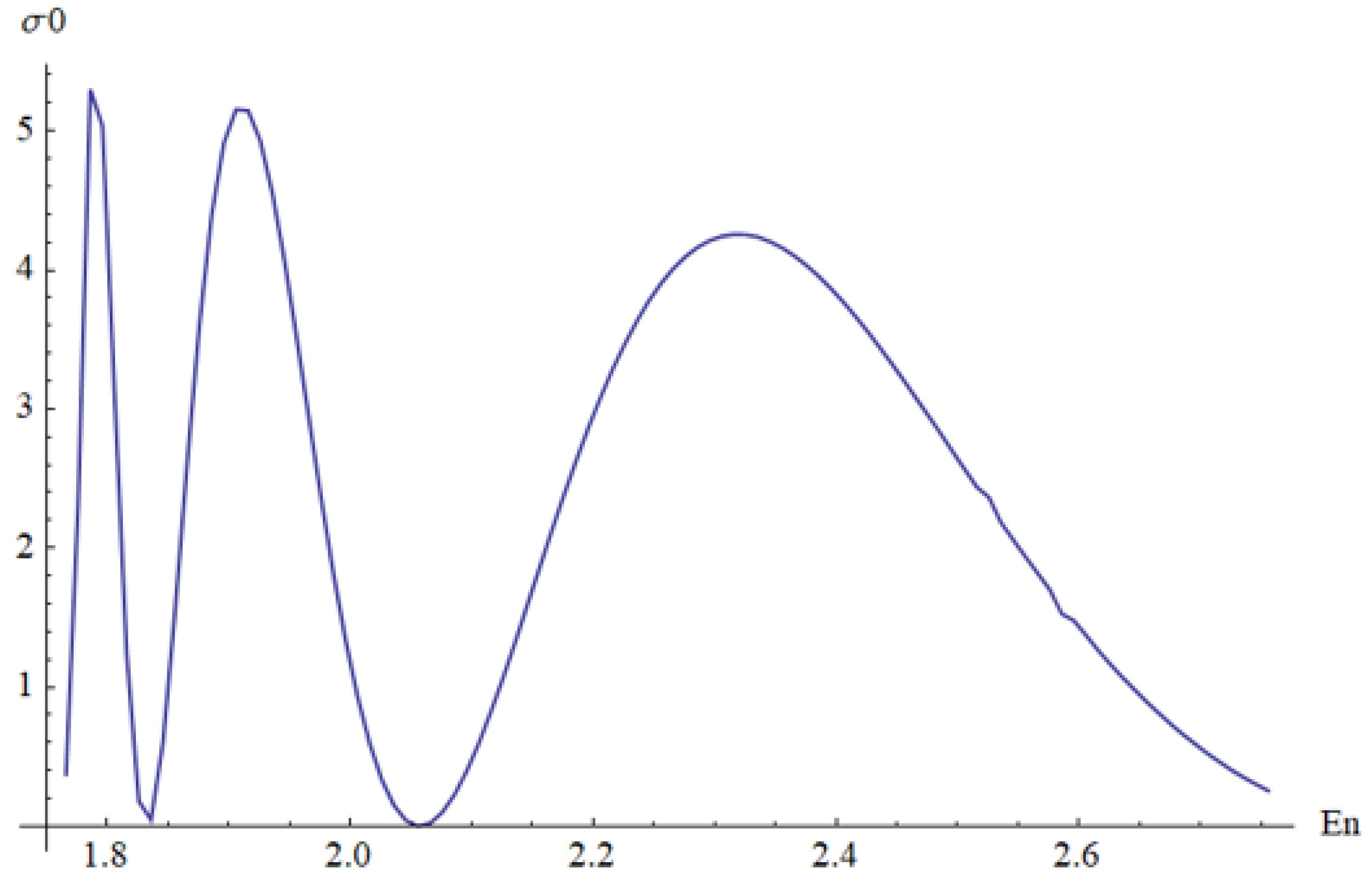
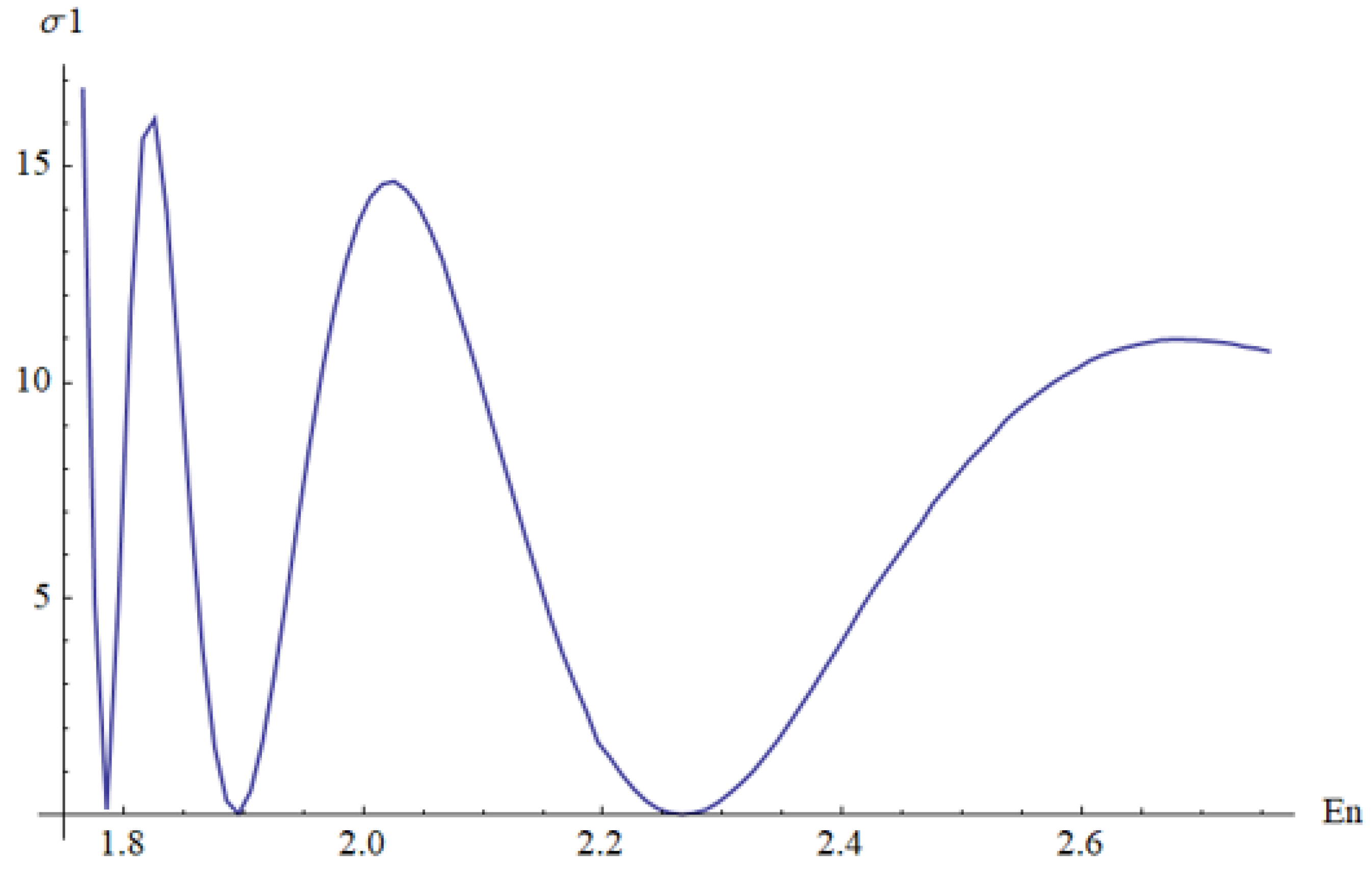
3. Scattering in the Cornell Potential

Now, we consider the case when the particle energy exceeds the value ${ϵ}_{max}/m$ (the case of scattering) and we determine the phase shifts ${\delta }_l\left(E\right)$ for given values of energy E and orbital quantum number l.

To do this, it is necessary to compare the numerical solution of Equation (7) at the end of the calculation segment with the solution of the approximate equation for $r⟶\infty$. The approximate equation is

$$\frac{d^{2}u}{d{r}^2}+2(ϵ-{ϵ}_{max})u=0,$$

where ${ϵ}_{max}$ is given by the Formula (13). In the case of scattering $ϵ>{ϵ}_{max}$ and under initial conditions (12), it has a solution of the form

$$u\sim sin\left(\sqrt{2(ϵ-{ϵ}_{max})}r\right).$$

For the numerical solution of Equation (7), we will choose an interval from $r_0=0.001Ge{V}^{-1}$ to $r_k$, which is several times larger than $r_c$, where $r_c$ is the distance from the origin at which $V_{eff}\left(x\right)\approx {ϵ}_{max}$ with a given accuracy (we took $\Delta =|V-{ϵ}_{max}|={10}^{-6}Ge{V}^2$). Then, the numerical solution of Equation (7) under the same initial conditions (12) at the end of the computational segment will have the form

$$u\sim sin(\sqrt{2(ϵ-{ϵ}_{max})}r+{\delta }_l\left(ϵ\right)).$$

The phase shift can be determined from the numerical solutions as

$${\delta }_l\left(ϵ\right)=\sqrt{2(ϵ-{ϵ}_{max})}(r_{1max}-r_{2max}),$$

where $r_{1max}$ and $r_{2max}$ are the positions of the maxima in the last period of the first and second solutions, respectively. The integral partial cross-section is then determined by the formula

$${\sigma }_l=\frac{4\pi }{\left(2ϵ\right)}(2l+1){sin}^2\left({\delta }_l\left(ϵ\right)\right),$$

(14)

Because in the selected units of measurement, $k^2=2ϵ$. Figure 5 and Figure 6 show the dependence of partial cross-sections on energy at $\rho =10Ge{V}^{-1}$ for $l=0$ and $l=1$.

Let us also consider the case of low-energy scattering at $l=0$. Let us study the dependence of the scattering length on the radius of curvature of Lobachevsky space. For each value of the radius of curvature, we will take an energy only slightly exceeding $ϵ/m$ (we took $E=ϵ/m+0.01GeV$), which meets the condition $E⟶ϵ/m$. These values are different for different $\rho$ (the energy that can be considered as “low” depends on the radius of curvature, i.e., it depends on the shape of the potential). Then, having determined the cross-section, using Formula (14), we find the scattering length as $L=\sqrt{{\sigma }_0/\left(4\pi \right)}$ and we study the dependence $L\left(\rho \right)$ (see Figure 7).

We see that the length of scattering varies significantly with the varying radius of curvature. For example, at $\rho \approx 2Ge{V}^{-1}$ the low-energy scattering cross-section reaches its maximum, while at $\rho \approx 3.5Ge{V}^{-1}$ it is zero (no scattering).

4. Conclusions

This paper shows that the Cornell potential in Lobachevsky space, contrary to the case of flat space, is a potential well of finite depth. Therefore, for particles moving in such a potential, both bound states and scattering states are possible. In this case, the greater the radius of curvature of Lobachevsky space and the smaller the quantum number of the orbital momentum, the greater the depth of the potential well. For values of the potential parameters typical of charmonium and an arbitrarily chosen radius of curvature, numerical solutions corresponding to bound states and their corresponding energy levels were found. It was shown that the number of bound states of the system increases with an increasing radius of curvature and decreases with increasing orbital quantum numbers. For the scattering problem, energy dependences were obtained for the first few partial cross-sections, as well as the dependence of the scattering length on the radius of curvature of the space. It is interesting to note that for some values of $\rho$ we had ${\sigma }_0=0$, which means that in Lobachevsky space with the particular radius of curvature a particle with zero angular momentum and with low energy is not scattered.

References

1. Friedman, A. Über die Krümmung des Raumes. Z. Phys. 1922, 10, 377–386. [Google Scholar] [CrossRef]
2. Friedmann, A. Über die Möglichkeit einer Welt mit konstanter negativer Krümmung des Raumes. Z. Phys. 1924, 21, 326–332. [Google Scholar] [CrossRef]
3. Friedmann, A. On the Curvature of Space. Gen. Relativ. Gravit. 1999, 31, 1991–2000. [Google Scholar] [CrossRef]
4. Friedmann, A. On the Possibility of a World with Constant Negative Curvature of Space. Gen. Relativ. Gravit. 1999, 31, 2001–2008. [Google Scholar] [CrossRef]
5. Tropp, E.A.; Frenkel, V.Y.; Chernin, A.D. Alexander A. Friedmann. The Man Who Made the Universe Expand; Dron, A.; Burov, M., Translators; Cambridge University Press: Cambridge, MA, USA, 1993. [Google Scholar]
6. Gliner, E.B. Algebraic properties of the energy-momentum tensor and vacuum-like states of matter. Sov. Phys. JETP 1966, 22, 378–382. [Google Scholar]
7. Jenkovszky, L.L.; Trushevsky, A.A. Asymptotics of total cross-sections and ultimate temperature of hadronic systems. Nuovo C. A 1976, 34, 369–384. [Google Scholar]
8. Bugrij, A.I.; Trushevsky, A.A. Some cosmological consequences of high-temperature phase transition in hadron matter. Astrofizika 1977, 13, 361–374. [Google Scholar]
9. Kokkedee, J. Theory of Quarks; Mir: Moscow, Russia, 1971; 338p. [Google Scholar]
10. Shelest, A.P.; Zinoviev, G.M.; Miranskij, V.A. Models of Strongly Interacting Particles; Atomizdat: Moscow, Russia, 1975; 232p. [Google Scholar]
11. Bykov, A.A.; Dremin, I.M.; Leonidov, A.V. Potential models of quarkonium. Sov. Phys. Uspekhi 1984, 27, 321. [Google Scholar] [CrossRef]
12. Sergeenko, M.N. Masses and widths of Resonances for the Cornell Potential. Adv. High Energy Phys. 2013, 2013, 325431. [Google Scholar] [CrossRef]
13. Izmestiev, A.A. Exactly solvable potential model for quarkoniums. Nucl. Phys. 1990, 52, 1697–1710. [Google Scholar]
14. Kudryashov, V.V.; Murzov, V.I.; Tomilchik, L.M. Triplet State of a Two-Fermion System with Homogeneous Relative Space; Preprint No. 568; B.I. Stepanov Institute of Physics, Academy of Sciences of the BSSR: Minsk, Russia, 1969; 19p. [Google Scholar]
15. Gamow, G. The Creation of the Universe; Viking Press: New York, NY, USA, 1952. [Google Scholar]
16. Gliner, E.B. Algebraic Properties of the Energy-momentum Tensor and Vacuum-like States o+ Matter. Sov. Phys. JETP 1965, 22, 378. [Google Scholar]
17. Gliner, E.B. Vacuum-like state of a medium and Friedmann cosmology. Dokl. Akad. Nauk USSR 1970, 192, 771–774. [Google Scholar]
18. Gliner, E.B.; Dymnikova, I.G. Nonsingular Friedmann cosmology. Sov. Astron. Lett. (Engl. Transl.) 1975, 1, 7. [Google Scholar]
19. Bugrij, A.I.; Trushevsky, A.A. Some cosmological consequences of the high-temperature hadron phase transition. Astrophysics 1977, 13, 195–202. [Google Scholar] [CrossRef]
20. Jenkovszky, L.L.; Kämpfer, B.; Sysoev, V.M. On the expansion of the universe during the confinement transition. Z. Phys. C 1990, 48, 147. [Google Scholar] [CrossRef]
21. Jenkovszky, L.L.; Kaempfer, B.; Sysoev, V.M. Bubble-free energy during the confinement transition. Phys. Atomic Nuclei 1994, 57. [Google Scholar]
22. Einstein, A. Kosmologiche Betrachtungen zur Allgemeinen Relativitätstheorie. Sitzungsberichte Königlich Preuss. Akad. Wiss. 1917, 1, 142. [Google Scholar]
23. Schrödinger, E. A method of determining quantum mechanical eigenvalues and eigenfunctions. Proc. R. Irish. Acad. A 1940, 46, 9–16. [Google Scholar]
24. Infeld, L. On a new treatment of some eigenvalue problems. Phys. Rev. 1941, 59, 737–747. [Google Scholar] [CrossRef]
25. Infeld, L.; Schild, A. A note on the Kepler problem in a space of constant negative curvature. Phys. Rev. 1945, 67, 121–122. [Google Scholar] [CrossRef]
26. Stevenson, A.F. A note on the Kepler problem in a spherical space, and the factorization method of solving eigenvalue problems. Phys. Rev. 1941, 59, 842–843. [Google Scholar] [CrossRef]
27. Higgs, P. Dynamical symmetries in a spherical geometry. J. Phys. A Math. Gen. 1979, 12, 309–323. [Google Scholar] [CrossRef]
28. Leemon, H. Dynamical symmetries in a spherical geometry. J. Phys. A Math. Gen. 1979, 12, 489–501. [Google Scholar] [CrossRef]
29. Kurochkin, Y.A.; Otchik, V.S. Analog of the Runge—Lenz vector and energy spectrum in the Kepler problem on a three-dimensional sphere. Dokl. AN BSSR 1979, 987–990. [Google Scholar]
30. Bogush, A.A.; Kurochkin, Y.A.; Otchik, V.S. On the quantum-mechanical Kepler problem in a three-dimensional Lobachevsky space. Dokl. AN BSSR. 1980, 19–22. [Google Scholar]
31. Kurochkin, Y.A.; Otchik, V.S.; Tereshenkov, V.I. Electron in a magnetic charge field in three-dimensional Lobachevsky space. Proc. Acad. Sci. BSSR Phys. Math. Ser. 1984, 74–79. [Google Scholar]
32. Kurochkin, Y.A.; Shoukavy, D.V. Regge trajectories of the Coulomb potential in the space of constant negative curvature 1S3. J. Math. Phys. 2006, 47, 022103. [Google Scholar] [CrossRef]
33. Muradian, R. The Regge law for heavenly bodies. Phys. Part. Nucl. 1997, 28, 471. [Google Scholar]
34. Trushevsky, A.A. Asymptotic Behavior of Boson Regge Trajectories. Ukr. J. Fiz. 2021, 97, 66. [Google Scholar] [CrossRef]
Figure 1. Effective potential plot.
Universe 10 00076 g001
Figure 2. Numerical solutions for the bound states and corresponding energy levels.
Universe 10 00076 g002
Figure 3. Number of bound states.
Universe 10 00076 g003
Figure 4. Regge trajectories.
Universe 10 00076 g004
Figure 5. Partial cross-section σ 0 ( E ) .
Universe 10 00076 g005
Figure 6. Partial cross-section σ 1 ( E ) .
Universe 10 00076 g006
Figure 7. Scattering length.
Universe 10 00076 g007
Disclaimer/Publisher’s Note: The statements, opinions and data contained in all publications are solely those of the individual author(s) and contributor(s) and not of MDPI and/or the editor(s). MDPI and/or the editor(s) disclaim responsibility for any injury to people or property resulting from any ideas, methods, instructions or products referred to in the content.