Statistical Study on the Q Parameter Based on Parkes Data

Abstract

Using the rotating vector model (RVM) and aiming to constrain the value of the magnetic inclination angle ($\alpha$), we perform a least-squares fit on the linearly polarized position angles of 125 pulsars from Parkes 64 m archive data at 1400 MHz. Subsequently, a statistical analysis of the normalized Q parameters is carried out. Furthermore, based on the Q-parameter, we provide a further understanding of the geometry of the radio emission region of the pulsar. In this statistical sample, about 1/5 of the sample is clustered at 0, suggesting that this part of the pulsar is viewed from the center of the radiation cone. For the rest of the pulsars, the Q parameters follow a uniform distribution, supporting the conclusion that the interface of the radiation cone is non-elliptical.

1. Introduction

Radio pulsars are thought to be rapidly rotating highly magnetized neutron stars. With the strong magnetic field unaligned with the axis of spin, periodical radio emission from the magnetosphere can be observed along the line of sight. As one of the most important properties, mean profiles with polarization can provide the fundamental understanding of the structure of the radio emission region, emission mechanism, and propagation process in the magnetosphere.

In 1976, Backer [1] proposed an empirical model of a “hollow-cone beam” after analyzing observational data from over fifty pulsars and categorized the average pulse profiles into five types: single peak, unresolved double peak, resolved double peak, triple peak, and multiple peaks. Following Backer’s empirical model, Rankin [2], in 1983, introduced the “core + double cone” model after analyzing observational data from over 100 pulsars, providing evidence for the existence of central components in the radiation beam. Further modification of this model has been added in the following studies. Olszanski et al. [3] studied the polarization characteristics and average pulse profiles of 46 pulsars observed with the Arecibo Telescope at 4.5, 1.5, and 0.3 GHz, revealing that nearly all the pulsars exhibited features that align with the core/double-cone emission beam model. In 2023, Rankin et al. [4] conducted a study using the Arecibo Telescope to analyze data from 58 pulsars observed at 1.4 GHz. The research focused on interpreting the geometric structures of the radiation zones and classifying the average pulse profile morphology. The geometric shape of the polar cap model proposed by Lyne and Manchester [5] (hereafter LM88) effectively describes the observed pulse position angle variations for some highly polarized pulsars. However, the linear polarization properties of pulsars can become complex due to the emergence of orthogonal emission modes, as discussed by Taylor and Manchester [6], Taylor et al. [7]. Brinkman et al. [8] conducted research on the polarization characteristics and pulse profiles at 327 MHz and 1400 MHz of 12 pulsars, which had previously not been extensively studied. The radiation cone structures of all core/double-cone model types of 76 pulsars were studied by Rankin et al. [4]. It was found that when the radiation energy was greater than or equal to ${10}^{32.5}erg{s}^{-1}$, they exhibited either core-single or core-cone triple patterns, while the remaining pulsars displayed single, double, or multi-peaked cone shapes.

In the study of Wu [9], a modulation was created from the polar cap geometric model proposed by LM88, adding the spherical triangle RQT (see in Figure 1). This relates the variation range of the linearly polarized position angle to the beam width. Figure 1 gives the improved polar cap geometric model presented by Wu [9]. As the line of sight intersects a single point P which moves across the arc ST as the pulsar rotates, the polarization position angle $\Delta \psi$ of linearly polarized radiation from P is determined by the angle between the plane formed by the magnetic field lines passing through P and the meridian plane at phase $\Delta \varphi$. Consequently, as the observer’s line of sight scans the arc ST during the pulsar’s rotation, the change in the linearly polarized position angle of the radio emission exhibits an S-shaped curve with longitude. The polar cap geometric model defines the relationship between the linearly polarized position angle $\psi$, magnetic inclination angle $\alpha$, the minimum angle $\beta$ between the line of sight direction and the magnetic axis, and the pulse phase $\varphi$.

In 2001, Han and Manchester [10] investigated the radiation beam structure of 87 pulsars at 1 GHz using the polar cap geometric model, The position traversed by the line of sight within the radiation cone was quantified using the normalized parameter ${\beta }_n$. This parameter (${\beta }_n$) is computed assuming $\alpha =90°$ as proposed by Lyne and Manchester [5]. Han’s study revealed that pulsars with ${\beta }_n$ values around 0.25 were most likely to exhibit multi-peaked pulse profiles, while the scarcity of pulsars with ${\beta }_n$ values near 0 might be attributed to observational biases [10], and only 1 to 2 pulsars with ${\beta }_n$ greater than 0.8.Therefore, there is a significant statistical uncertainty in the average profile shape within these intervals. In 2015, Rankin [11] conducted polarization measurements of 33 pulsars using the Green Bank Telescope. The rotating vector model (RVM), originally proposed by Radhakrishnan and Cooke [12], was employed to fit the magnetic inclination angles. ${\beta }_n$ values were derived for 12 of these pulsars, exhibiting a somewhat scattered distribution. However, due to the limited sample size, no further research was conducted on the distribution of ${\beta }_n$ [13].

This study is based on Parkes observations [14], and the dataset is also available in the European Pulsar Network Data Archive (EPN) 1. Using the magnetic pole cap geometry model, the geometric parameters of pulsars are fitted by the least square method, and the radiation characteristics and the geometric structure of the pulsar’s emission region are studied in detail. In particular, according to the rotation vector model proposed by Radhakrishnan and Cooke [12], pulsars with a more complete S-shaped position angle have more complete polarization information and emission region information. In this study, we obtained 125 samples with relatively complete S-shaped position angles from the 600 pulsars at 1400 MHz observed by Johnston using Parkes in 2018. With the fitting results based on the polar cap geometry model, the normalized parameter Q representing the line-of-sight position relative to the emission cone is calculated. The distribution of the parameter Q will be further investigated under a large number of samples.

This paper is organized as follows: Section 2 provides an introduction to the investigation of the Q parameter, involving the utilization of the least-squares method to fit the geometric parameters of the radiation region, the derived results are then utilized to solve for the Q parameter; Section 3 mainly describes the distribution of the Q parameter; Section 4 classifies the average pulse profiles and explains the distribution of the Q parameter for different pulse shapes; Section 5 provides the final discussion and conclusion.

2. The Calculation of Q Parameter

2.1. Research on Q Parameter and ${\beta }_n$

The parameter $\beta$ typically represents the position of the radiation cone during line of sight scanning, while it cannot be directly determined from observations. Moreover, the value of $\beta$ does not directly indicate the angular distance of the line of sight to the magnetic axis. Different works have defined similar parameters. Narayan and Vivekanand [15] gave the parameter y/r, where y is the angular deviation in latitude between the line of sight and the magnetic pole, and r stands for the radius of the beam. Malov [16,17] introduced the parameters n and $\chi =1/n$, which determine the minimum angular distance of the line of sight from the center of the cone of open field lines. Their work calculated the n parameters of 35 pulsars at 400 MHz and revealed that in pulsars with complex pulse profiles, the line of sight primarily traverses through the central region, whereas in pulsars with one-component profiles, the line of sight scans along the edges.

Lyne and Manchester [5] defined ${\beta }_n={\beta }_{90}/{\rho }_{90}$ as the normalized impact parameter when the magnetic inclination angle $\alpha$ is 90° in 1988. Equations (2) and (3) give the ${\beta }_{90}$ and ${\rho }_{90}$, where $\Delta \varphi$ is represented by $W_{10}$, $10\%$ of the peak intensity. Their work provided the distribution of ${\beta }_n$ for 128 pulsars around 400 MHz, showing a deficit at relatively high ${\beta }_n$ values, which may be attributed to observational or selection effects.The following study [10] extrapolated a similar distribution at 1 GHz.

${\beta }_n$ is calculated based on the ratio of ${\beta }_{90}$ and ${\rho }_{90}$ when $\alpha$ is 90°. Unlike ${\beta }_n$, Wu et al. [18] established a normalized parameter Q, which is independent of $\alpha$ (see Equation (1)), that effectively represents the position of the line of sight cutting the beam at the center of the cone.

$$\begin{array}{cc}\hfill \mathrm{Q}& =\frac{\beta }{\rho }.\hfill \end{array}$$

(1)

For the aim of describing the location where the line of sight cuts the radiating cone, the Q parameter proves to be more specific than $\beta$. Q = 0 indicates that the line of sight sweeps through the center of the radiating cone, while Q = 1 signifies that it sweeps through the edge of the cone [19]. Wu and Gil [20] conducted a study that focused on 58 pulsars near 400 MHz. They examined the radiation characteristics and geometric structures of the pulsar emission regions using the Q and $\rho$-P relationship, which is an empirical relationship discovered by Kuz’min et al. [21].

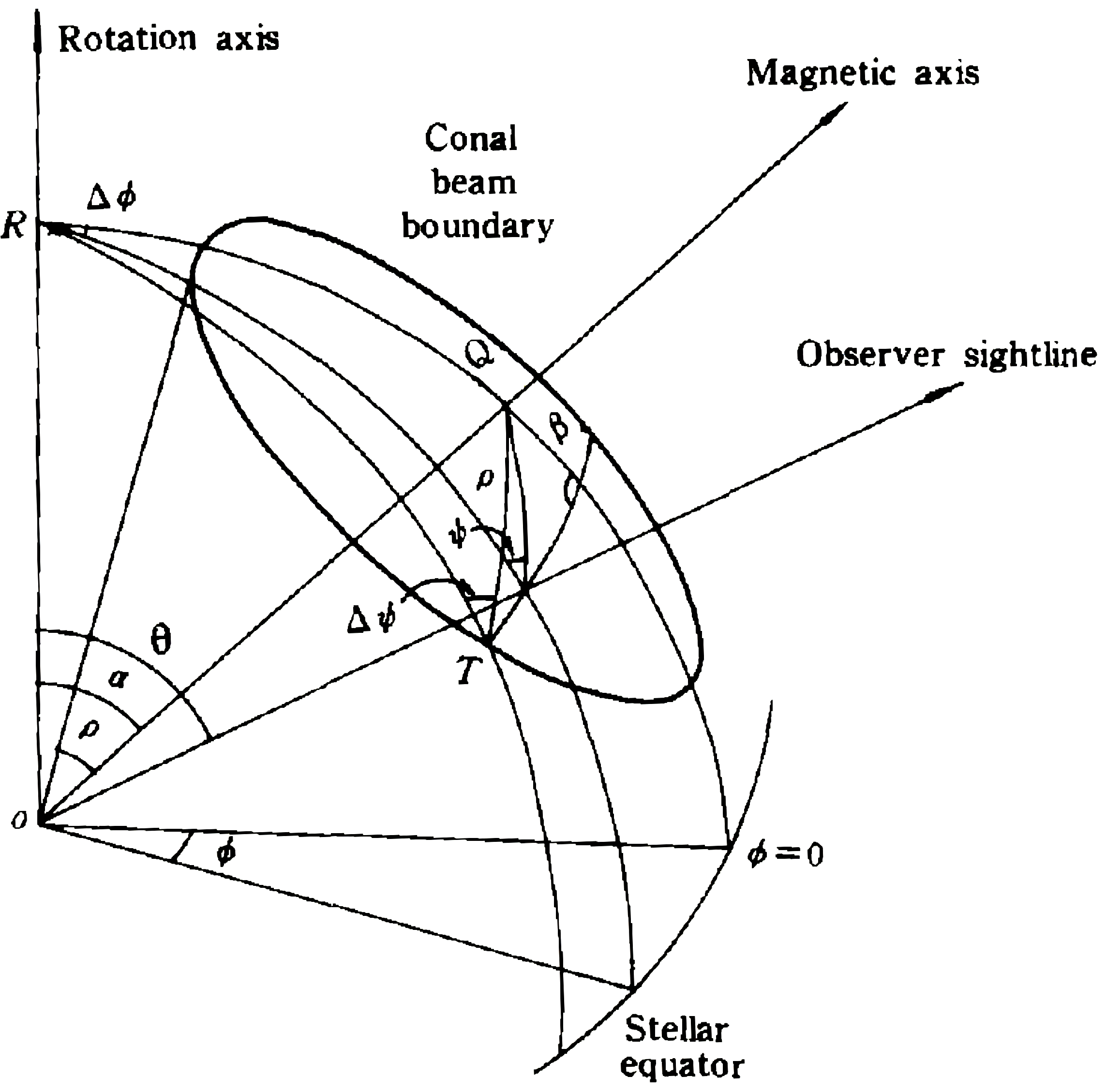
2.2. The Calculation of Geometric Parameters $\alpha$, $\beta$, and $\rho$

The geometric relationships of the polar cap model differ in the number of unknown parameters. Gould [22], Wu [9], and Lyne and Manchester [5] employed a method involving the introduction of new relationships to solve for the magnetic inclination angle. A rotation vector model is utilized to fit the position angle curve of the pulsar. In this model (see Figure 1), the observed position angle is defined by the following equation.

By considering the relationships between arcs and angles within the spherical triangle RQP, the following relationships can be obtained:

$$tg\left(\psi -{\psi }_0\right)=\frac{sin\alpha sin\varphi }{sin\zeta cos\alpha -cos\xi sin\alpha cos\varphi },$$

(2)

$$si{n}^2\left(\frac{\varrho }{2}\right)=si{n}^2\left(\frac{\Delta \varphi }{2}\right)sin\alpha sin(\alpha +\beta )+si{n}^2\left(\frac{\beta }{2}\right),$$

(3)

$$tan\Delta \psi ={(d\psi /d\varphi )}_{m}sin\Delta \varphi .$$

(4)

The spherical triangle RQT exhibits angle–arc relationships:

$$cos\Delta \varphi =\frac{cos\rho -cos\alpha cos\zeta }{sin\alpha sin\zeta },$$

(5)

$$\Phi ={\left(\frac{d\psi }{d\varphi }\right)}_{max}=\frac{sin\alpha }{sin\beta },$$

(6)

$$tg\Delta \psi =\frac{sin\Delta \varphi sin\alpha }{cos\alpha sin\zeta -cos\zeta sin\alpha cos\Delta \varphi }.$$

(7)

where $\Delta \varphi =\varphi -{\varphi }_0$, with ${\varphi }_0$ representing the pulse phase at the maximum gradient of the position angle variation, and $\Delta \psi =\psi -{\psi }_0$, with ${\psi }_0$ denoting the linearly polarized position angle at the pulse phase ${\varphi }_0$; $\alpha$ is the magnetic inclination angle, $\rho$ is radiation cone angle, and $\beta$ is minimum angle between the line of sight and the magnetic axis. The inclination of the observer direction to the rotation axis is $\zeta =\alpha +\beta$. Wu et al. [19] and Lyne and Manchester [5] independently derived a relationship among the observational parameters of three coronal geometry models:

$$tg\Delta \psi \approx \Phi sin\Delta \varphi .$$

(8)

There are three parameters in the magnetic-pole model: $\alpha$, $\rho$, and $\beta$, while only two independent equations and two observable quantities ($\Delta \varphi$ and $\Delta \psi$, see Equation (3)), were obtained from the arc–angular relationship in the model. This means the determination of a parameter or a new relationship is necessary. Using Equation (1) and the statistical relationship $\rho \text{-}P$, Kuz’min et al. [21], Kuz’min [23] gave the numerical values of $\alpha$, $\beta$, and $\rho$ for 56 and 105 pulsars, respectively. Similarly, LM88 developed a new statistical method to acquire an updated $\rho \text{-}P$ relationship and obtained the values of the three parameters.

In our study, we listed all the $\alpha$s from $0°$ to $90°$ with a step of $0.1°$ and then calculated the corresponding two parameters $\beta$ and $\rho$ using Equations (5) and (7). The three parameters($\alpha$, $\beta$, and $\rho$) need to be determined in a least-squares-fit analysis of polarization position angle. The goodness of fit is given by the the chi-squared test:

$${\chi }^2=\sum \frac{{(f_o-f_e)}^2}{f_e}.$$

(9)

The parameter calculated from Equation (8) is closely tied to the observed data, underscoring the need for careful consideration in selecting pulsar data parameters $\Delta \psi$ and $\Delta \varphi$ to ensure a robust statistical sample. As $\Delta \psi$ and $\Delta \varphi$ are functions dependent on frequency, it is imperative to choose observational data with closely matching frequencies. Additionally, the pronounced depolarization effect on the two sides of the average pulse profile and the limitations posed by the signal-to-noise ratio make obtaining accurate values for $W_{10}$ particularly challenging. Given the incomplete or distorted nature of the linear polarization position angle on both edges of the profile for most pulsars, it is prudent to include $W_{50}$ (the angular width at the $50\%$ peak intensity of the average pulse profile) and $\Delta \psi$ (the range of polarization position angle variation). Adhering to these principles, the chosen observational data for this study are available through the EPN at 1400 MHz. A total of 125 pulsars exhibiting an “S”-shaped polarization position angle with the longitude were selected from a dataset comprising 600 pulsar observations from Johnston and Kerr [14]. These pulsars exhibit strong linear polarization, present a continuous “S”-shaped variation in linear polarization position angle, and demonstrate favorable signal-to-noise ratios. Figure 2 and

Table 1. The data of four pulsars. The first column represents the name of the pulsar, the second column represents the period, the third column represents “$\Delta \varphi$”, the fourth column represents the magnetic inclination angle, and the fifth column represents the minimum distance “$\beta$” from the line of sight to the magnetic axis.

PSRJ	P (ms)	$\mathbf{\Delta }\mathit{\varphi }\mathbf{(}\mathbf{°}\mathbf{)}$	$\mathit{\alpha }\mathbf{(}\mathbf{°}\mathbf{)}$	$\mathit{\beta }\mathbf{(}\mathbf{°}\mathbf{)}$
J0614+2229	335.0	6.7	40.4	3.22
J1701-3726	2454.6	6.0	87.2	2.58
J1822-2256	1874.3	8.4	0.3	0.07
J1835-1106	165.9	8.4	0.3	3.06

give the example fitting results of four pulsars (PSRs J0614+2229, J1701−3726, J1822−2256, J1835−1106). Notably, the fitting curves obtained using the least squares method showcase a remarkable agreement with the observed curves at different magnetic inclination angle values.

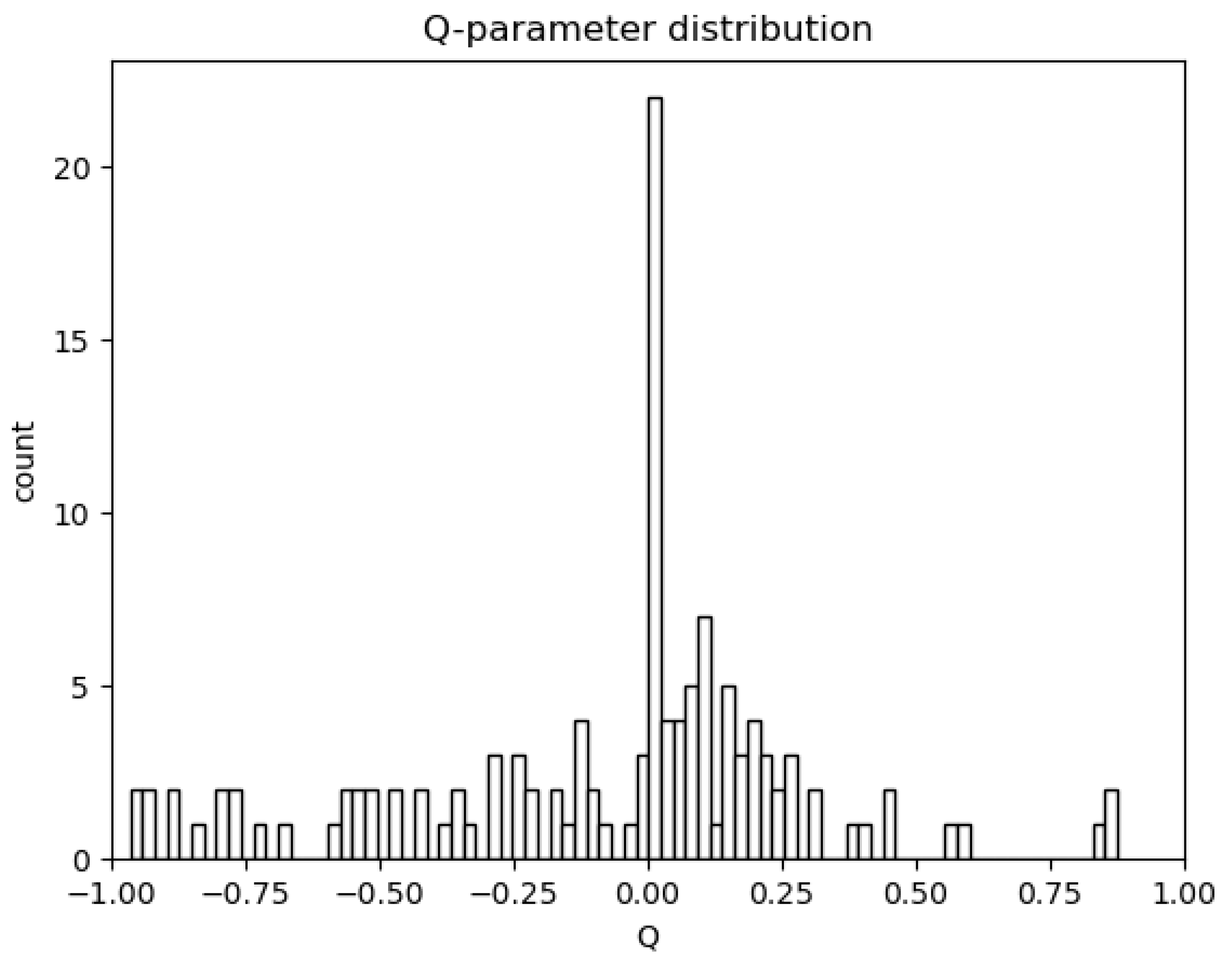
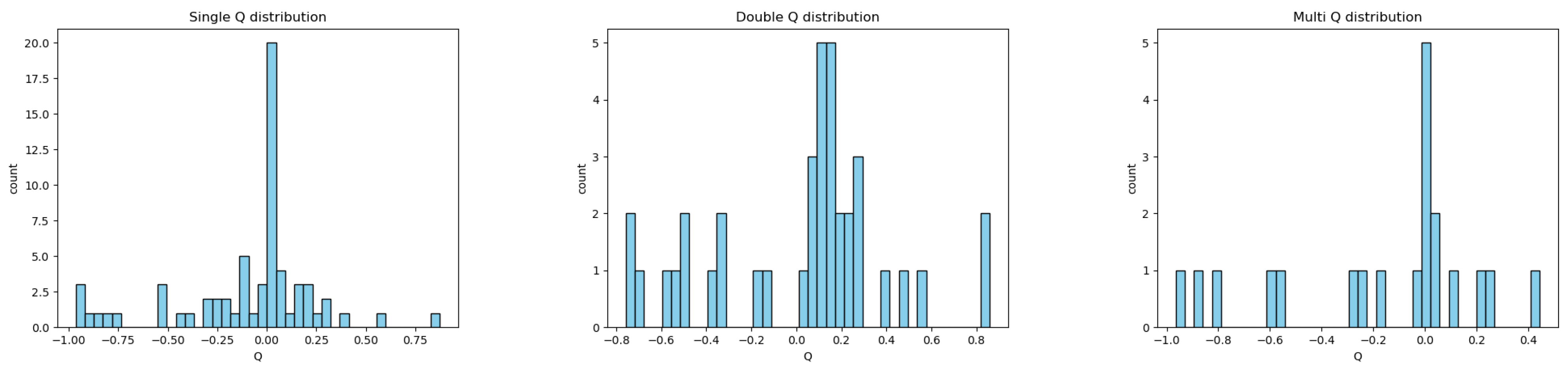
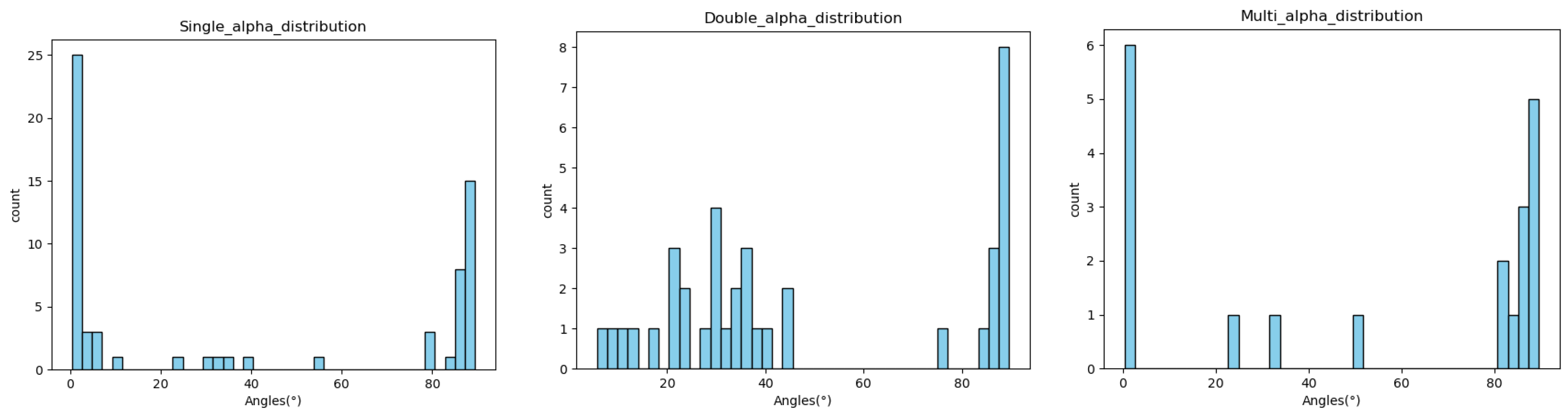
3. Distribution of Q Parameter

Through a fitting analysis of the selected pulsar dataset, we successfully derived the geometric parameters for a total of 125 pulsars. Simultaneously, employing Equation (1) enabled us to compute the Q parameters for this set of stars. The corresponding parameter values can be found in

Table 2. Pulsar parameter table of 125 pulsars. The first column represents the name of the pulsar; the second column represents the period; the third column represents “$\Delta \varphi$”; the fourth column represents the magnetic inclination angle; the fifth column represents the minimum distance “$\beta$” from the line of sight to the magnetic axis; the sixth column represents “$\rho$”; the seventh column represents the “Q” parameter; and the eighth column represents the Number of peaks in the average pulse profile. The table uses “S” to signify a pulsar displaying a single-peaked pulse profile, “D” to denote a pulsar exhibiting a double-peaked pulse profile, and “M” to represent a pulsar with a triple-peaked or multi-peaked pulse profile.

PSRJ	P (ms)	$\mathbf{\Delta }\mathit{\varphi }\mathbf{(}\mathbf{°}\mathbf{)}$	$\mathit{\alpha }\mathbf{(}\mathbf{°}\mathbf{)}$	$\mathit{\beta }\mathbf{(}\mathbf{°}\mathbf{)}$	$\mathit{\rho }\mathbf{(}\mathbf{°}\mathbf{)}$	Q	Class
J0108-1431	807.6	11.6	1.1	1.43	8.568	0.166	S
J0134-2937	137.0	4.9	1.3	0.15	20.803	0.007	S
J0304+1932	1387.6	10.9	87.0	−3.15	6.536	−0.481	D
J0525+1115	354.4	14.1	88.6	−3.05	12.934	−0.235	M
J0528+2200	3745.5	14.6	30.0	0.88	3.979	0.221	D
J0536-7543	1245.9	16.5	89.5	−3.30	6.898	−0.478	D
J0601-0527	396.0	14.4	23.5	6.90	12.236	0.563	D
J0614+2229	335.0	6.7	40.4	3.22	13.304	0.242	S
J0624-0424	1039.1	1.8	98.6	−0.92	7.554	−0.121	D
J0631+1036	287.8	8.1	84.9	3.19	14.353	0.222	M
J0729-1448	251.7	12.0	12.6	1.46	15.348	0.095	D
J0729-1836	510.2	3.9	7.8	0.85	10.780	0.078	D
J0742-2822	166.8	9.1	89.3	−10.75	18.854	−0.570	M
J0745-5353	214.8	17.9	85.5	−9.01	16.614	−0.542	S
J0904-7459	549.6	10.9	33.1	3.32	10.384	0.319	S
J0905-5127	346.3	7.7	36.6	1.26	13.085	0.096	D
J0907-5157	253.6	17.2	0.4	0.29	15.290	0.018	M
J0922+0638	430.6	4.9	5.1	2.17	11.734	0.184	S
J0940-5428	87.5	10.5	20.8	5.99	26.031	0.230	D
J0942-5552	664.4	4.9	0.9	0.17	9.447	0.017	M
J0942-5657	808.1	1.8	0.7	0.04	8.566	0.004	S
J0954-5430	472.8	7.4	26.9	1.71	11.198	0.152	D
J0959-4809	670.1	50.6	10.3	1.94	9.406	0.206	D
J1048-5832	123.7	14.1	33.8	5.66	21.893	0.258	D
J1105-6107	63.2	3.1	88.1	−3.10	30.628	0.121	D
J1057-5226	197.1	162.1	0.5	0.23	17.344	0.013	M
J1110-5637	558.3	13.0	34.6	0.68	10.305	0.065	D
J1115-6052	259.8	5.6	87.1	−14.58	15.106	−0.965	S
J1119-6127	408.0	19.0	89.5	−5.1	12.055	−0.423	S
J1141-3322	291.5	13.4	0.7	0.03	14.262	0.002	M
J1202-5820	452.8	7.0	30.0	0.98	11.443	0.0856	D
J1216-6223	374.0	10.2	1.4	0.40	12.591	0.031	S
J1224-6407	216.5	9.1	35.3	2.99	16.549	0.180	D
J1253-5820	255.5	4.9	1.0	0.10	15.233	0.006	S
J1301-6305	184.5	43.6	1.5	1.38	17.926	0.076	S
J1320-3512	58.5	7.7	2.1	0.09	11.372	0.007	S
J1326-6408	792.7	3.5	82.9	−8.35	8.648	−0.965	M
J1326-6700	543.0	27.8	23.6	2.79	10.449	0.267	D
J1338-6204	1239.0	26.0	81.7	−5.56	6.918	−0.803	M
J1356-5521	507.4	10.9	1.0	0.12	10.810	0.011	S
J1357-6429	166.1	27.4	0.8	0.60	18.893	0.032	S
J1359-6038	127.5	7.0	4.2	1.58	21.564	0.073	S
J1420-6048	68.2	45.0	45.2	8.00	29.485	0.271	D
J1452-5851	386.6	7.0	78.8	−9.49	12.384	−0.766	S
J1507-4352	355.7	2.8	88.0	−2.86	12.911	−0.221	S
J1512-5759	128.7	13.7	1.8	0.01	21.464	0.001	S
J1513-5908	151.3	34.5	1.2	1.32	19.796	0.066	S
J1522-5829	395.4	12.0	88.8	−1.65	12.245	−0.134	S
J1524-5625	78.2	36.6	5.7	2.61	27.535	0.094	D
J1524-5706	1116.0	4.6	1.0	0.09	7.289	0.012	S
J1530-5327	279.0	10.2	30.9	1.99	14.578	0.1365	D
J1535-4114	432.9	12.3	16.3	1.80	11.703	0.153	D
J1549-4848	288.3	7.4	54.3	−3.44	14.341	−0.239	S
J1551-5310	453.4	26.4	5.3	6.73	11.435	0.588	S
J1557-4258	329.2	4.2	32.2	1.35	13.420	0.100	M
J1600-5044	192.6	8.1	1.0	0.10	17.545	0.005	S
J1601-5335	288.5	7.4	3.2	0.09	14.336	0.006	S
J1614-5048	231.7	13.0	80.3	14.00	15.997	0.875	S
J1632-4757	228.6	26.7	0.5	0.25	16.105	0.015	S
J1633-4453	436.5	6.3	4.6	2.29	11.655	0.196	S
J1633-5015	352.1	6.3	1.6	0.92	12.977	0.070	S
J1636-4440	206.6	17.6	89.4	−1.44	16.940	−0.085	S
J1637-4553	118.8	9.5	1.9	0.26	22.340	0.011	S
J1643-4505	237.4	9.8	87.4	−8.20	15.803	−0.518	S
J1644-4559	455.1	6.3	0.3	0.09	11.414	0.007	S
J1646-4346	231.6	16.9	83.2	−14.89	16.000	−0.930	S
J1651-4246	844.1	43.6	89.3	−6.36	8.381	−0.758	D
J1651-5222	635.1	9.1	88.7	−1.15	9.662	−0.119	S
J1651-5255	890.5	8.4	86.3	−2.79	8.160	−0.341	D
J1651-7642	1755.3	15.5	21.5	2.65	5.812	0.455	D
J1700-3312	1358.3	8.4	30.0	0.70	6.607	0.105	D
J1701-3726	2454.6	6.0	87.2	−2.58	4.914	−0.524	D
J1701-4533	322.9	20.4	88.0	−9.25	13.551	−0.682	D
J1702-4128	182.1	19.7	88.3	−6.64	18.044	−0.367	S
J1705-1906	299.0	185.6	88.7	−4.87	14.082	−0.345	D
J1705-3423	255.4	6.5	85.9	−12.7	15.236	−0.833	S
J1709-1640	653.1	4.2	85.9	−1.01	9.528	−0.106	S
J1709-4429	102.5	20.0	6.0	2.25	24.051	0.093	S
J1715-3903	278.5	7.0	88.8	−4.27	14.591	−0.292	S
J1718-3825	74.7	7.7	23.2	6.60	28.173	0.234	M
J1722-3207	477.2	3.9	76.7	−1.94	11.147	−0.174	D
J1723-3659	202.7	12.3	88.6	−15.15	17.103	−0.885	S
J1730-3350	139.5	18.3	87.5	−3.06	20.616	−0.148	S
J1731-4744	829.8	7.4	89.4	−6.10	8.453	−0.721	D
J1739-3023	114.4	9.1	2.1	−0.94	22.766	−0.041	S
J1739-3131	529.4	14.1	89.3	−1.23	10.583	−0.116	S
J1740-3015	606.9	1.4	87.5	−2.33	9.884	−0.235	S
J1740+1000	154.1	19.7	45.0	8.13	19.615	0.414	D
J1740+1311	803.1	11.6	87.6	−2.50	8.592	−0.290	M
J1741-0840	2043.1	10.2	50.2	2.40	5.387	0.445	M
J1741-3927	512.2	7.4	88.5	0.06	10.759	0.005	S
J1749-3002	609.9	24.6	86.9	−1.68	9.860	−0.170	M
J1752-2806	562.6	3.9	85.7	−2.34	10.266	−0.227	S
J1757-2421	234.1	14.8	30.0	2.26	15.914	0.142	D
J1801-2154	375.3	8.1	86.9	−10.11	12.569	−0.804	S
J1801-2451	124.9	13.4	87.0	−11.75	21.788	−0.539	S
J1803-2137	133.7	35.2	85.5	1.06	21.058	0.050	M
J1803-2712	334.4	18.3	0.9	0.19	13.316	0.014	M
J1812-1733	538.3	43.6	86.0	−1.01	10.495	−0.096	S
J1812-2102	1223.4	12.0	88.3	−3.93	6.961	−0.564	D
J1815-1738	198.4	11.6	0.7	0.34	17.287	0.019	S
J1817-3618	387.0	8.4	0.6	0.05	12.378	0.004	S
J1820-0427	598.1	6.3	2.4	2.06	9.956	0.206	S
J1822-2256	1874.3	8.4	0.3	0.07	5.624	0.012	S
J1825-0935	769.0	4.6	84.3	0.42	8.781	0.0478	D
J1828-1101	72.1	45.4	79.8	−0.17	28.676	−0.005	S
J1835-0944	145.3	14.8	86.4	−0.27	20.200	−0.0133	M
J1835-1020	302.4	6.0	88.7	−3.98	14.002	−0.284	S
J1835-1106	165.9	8.4	0.3	3.06	18.905	0.161	S
J1841-0345	204.1	19.7	23.5	6.50	17.044	0.381	S
J1841-0425	186.1	8.4	88.7	−16.45	17.850	−0.921	S
J1842-0359	471.6	54.8	20.9	1.81	11.213	0.161	D
J1844-0538	273.0	10.2	35.9	4.53	14.737	0.307	S
J1852-0635	524.2	54.8	88.5	−9.33	10.635	−0.877	M
J1901-0906	1781.9	8.4	31.4	1.11	5.768	0.192	S
J1901+0413	2663.1	12.3	39.6	4.06	4.718	0.860	D
J1904+0004	139.5	18.3	1.0	0.43	20.616	0.021	S
J1905+0709	643.2	17.9	0.6	0.10	9.601	0.010	S
J1914+0219	457.5	10.5	89.6	−6.62	11.384	−0.581	M
J1917+1353	194.6	7.0	89.5	−6.31	17.455	−0.361	D
J1919+0134	1604.0	9.1	36.6	5.06	6.080	0.832	D
J1935+2025	80.1	8.8	10.2	1.07	27.207	0.039	S
J2006-0807	580.9	48.5	0.8	0.25	10.103	0.024	M
J2048-1616	1961.6	11.5	40.9	1.00	5.490	0.390	M
J2053-7200	341.3	25.7	37.9	1.41	13.180	0.106	D

, facilitating a comprehensive exploration of the distribution characteristics of the Q parameter.

Figure 3 shows the distribution of the normalized parameter Q, indicating the position of line of sight cutting through the radiating cone for each pulsar. The Q parameters of 1/5 of the samples are near 0, and the distribution of the rest is closer to the uniform distribution, indicating the rounded radiation cone, which is consistent with the results in Radhakrishnan and Cooke [12], Wu and Shen [24], and Lyne and Manchester [5]. Q parameters close to 0 indicate that the line of sight passed through the center of the cone of radiation more often in our sample. The luminosity, the selection effect of the observations, and the inadequate number of statistical sampling may account for this distribution. The observed flux density varies significantly as the sight-line traverses different regions of the radiating cone. Given that the energy distribution of pulsars within the radiating cone is highest at the center, there are more pulsars observed when the sight-shape passes through the center of the cone compared to other parts of the cone.

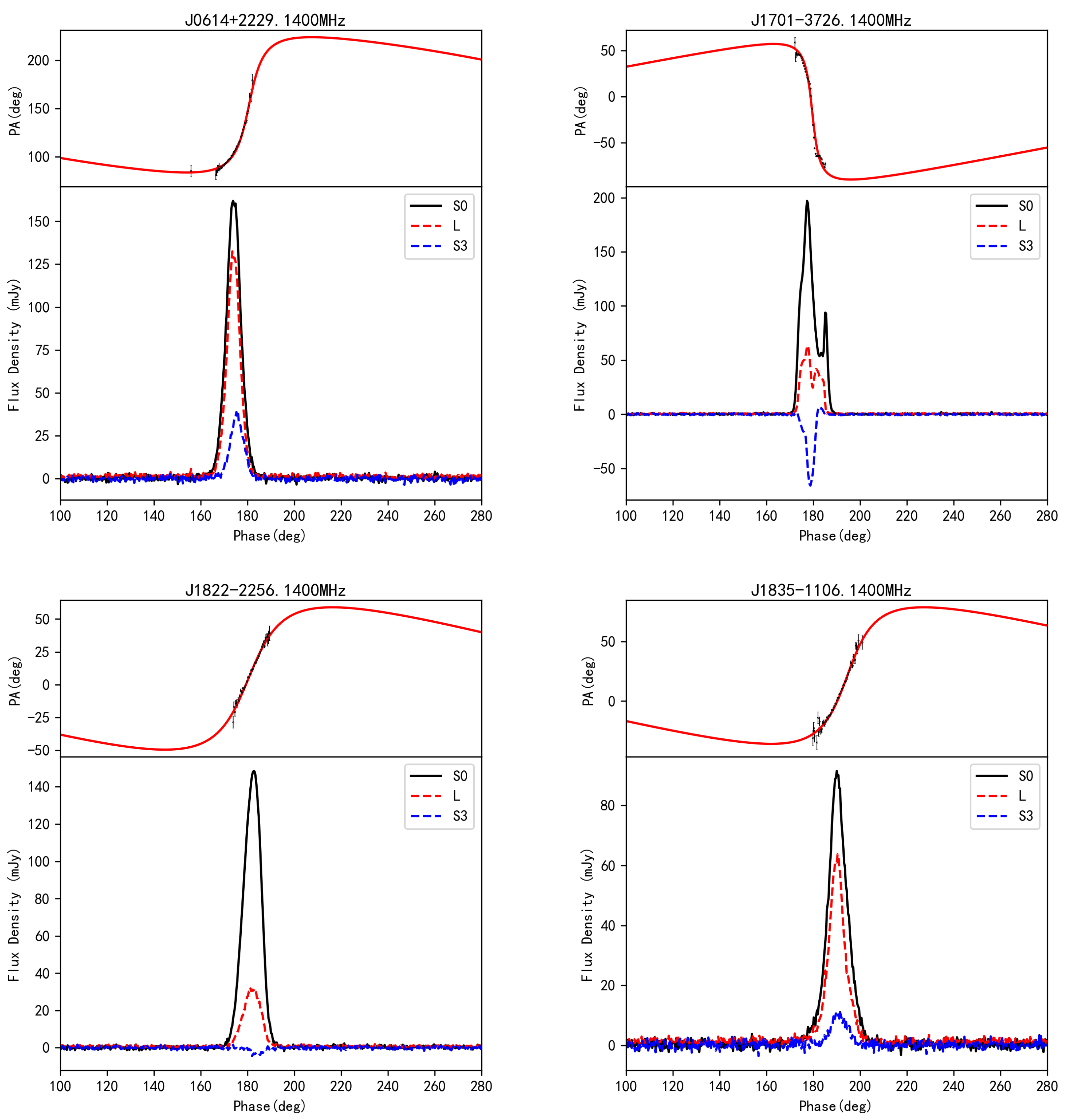
4. The Q Parameter and the Average PULSE Profile

Based on an analysis of multi-frequency polarization observation data from 100 pulsars, Rankin [2] developed a radiation zone geometric structure model known as “core + cone”. This model provides a comprehensive understanding of the existence and radiation characteristics of core components in the radiation beam. Furthermore, by using this model, the study successfully explains the occurrence of various types of average pulse profiles, such as single-peaked, double-peaked, and multi-peaked profiles. The research also investigates the distribution of magnetic $\alpha$ in single-peaked and multi-peaked profiles across 110 pulsars. The findings reveal that for single-peaked profiles, $\alpha$ is distributed between $15°$ and $90°$, with a peak at approximately $35°$. In contrast, multi-peaked profiles exhibit a wider distribution of $\alpha$ values, reaching a minimum of $3°$. Interestingly, similar to single-peaked profiles, multi-peaked profiles also show a peak at around $35°$ and a second peak near $90°$.

In the present study, we employed the “core + cone” model (Rankin [25,26]) to classify the average pulse profile types of 125 chosen pulsars. These profile types primarily fall into three categories: single-peaked, double-peaked, and multi-peaked. Table 2 provides the relevant data information and classifications for this sample of pulsars. A statistical analysis was performed to examine the distribution of the Q parameter across different profile types. The distribution of Q parameters for different average pulse profile classifications is presented in Figure 4. We found that the Q parameter distribution for single-peaked profiles is centered around $0°$. Similarly, double-peaked profiles exhibit a peak around $0°$ but with a more scattered distribution, while the Q parameter distribution for multi-peaked profiles is broader, ranging from −1 to 1. Figure 5 showcases the distribution of pulsar $\alpha$ across these classifications. In the case of single-peaked pulsars, the distribution of $\alpha$ values reveals the presence of two peaks, approximately centered at $4°$ and $88°$, within the range of $0°$ to $90°$. Similarly, multi-peaked profiles display peaks in the $\alpha$ distribution near $5°$ and $85°$, although the distribution range is wider compared to single-peaked profiles. For double-peaked pulsars, a peak can be observed around $30°$ in the $\alpha$ distribution.

5. Discussion and Conclusions

As a kind of extremely compact objects, pulsars are closely related to many interesting phenomena [27]. Employing the magnetic polar cap geometry model as the foundation, this study utilized the rotating vector model to conduct a least-squares fitting of the position angles of linear polarization observed at 1400 MHz for 125 pulsars. The fitting process incorporated a constraint on the magnetic inclination angle $\alpha$, resulting in the determination of possible geometric parameters in the emission regions of this pulsar sample. An examination of the fitted magnetic inclination angle $\alpha$ and the resulting fits indicates a close agreement between the fitted curve and the observational data points. This consistency demonstrates the reliability of our fitting approach.

The distribution of the Q parameter in this study is illustrated in Figure 3. Possible factors contributing to this distribution include observational effects, uncorrected radio brightness, and limited sample size. The impact of observational effects is primarily twofold. First, significant variations in flux density occur as the line of sight traverses different regions of the radiation cone, with the flux density at the edge of the cone being much lower than at the center [28]. Second, due to limitations in telescope precision and other factors, only pulsars with flux densities above a specific threshold can be detected. For pulsars with sightlines crossing the outer boundary of the radiation cone, the flux density could potentially drop below the detectable threshold of the telescope, thereby causing an absence of discernible pulse signals.

The radio luminosity-corrected formula proposed in this study was used to consider whether the radio luminosity will affect the Q parameter distribution, and the extent of its possible influence was determined according to the available data. The formula selected below (Equations (10)–(13)) was further modified by Wu et al. [18], Wu and Xu [29] on the basis of Taylor et al. [7].

$$L_R={\pi }^3\frac{W_E}{P}{d}^2{S}_{400}\Delta f.$$

(10)

$$L_{new}=L_R{K}_1{K}_2.$$

(11)

$$K_1={\left(\rho {/}_{\Delta {\varphi }_E}\right)}^2.$$

(12)

$$K_2=exp\left(\frac{\pi Q^2}{4(1-Q^2)}\right).$$

(13)

The correction factors $K_1$ and $K_2$ can be calculated using polarimetric data. $K_1$ is determined by the ratio of the radiation cone angle to the viewing beam width and can be greater than or less than 1. On the other hand, $K_2$, determined by the Q parameter, is designed to correct for errors arising from the sightline not passing through the center of the radiation cone, and it always exceeds 1.

The parameter Q is distributed within the range of 0 to 1. In cases of high extremity, when Q takes the value of 0.9, the corresponding $K_2$ value reaches 28.45, indicating that the sightline sweeps near the edge of the radiation cone. In such instances, the observer only detects a small fraction of the cone’s total energy. As Q decreases to 0.8, the $K_2$ value increases to 4.04, resulting in substantial errors. Furthermore, when Q drops to 0.5, the $K_2$ value decreases to 1.299, indicating the need for adjustments in the radio luminosity. Out of the provided sample of 125 pulsars, 25 pulsars exhibit Q values above 0.5, while 2 pulsars have Q values that surpass 0.9. As a result, we intend to conduct a statistical analysis on data from a larger sample of pulsars showing an S-shaped polarization position angle, which we anticipate will yield more robust statistical outcomes.

References

1. Backer, D. Pulsar Average Waveforms and Hollow Cone Beam Models; Technical Report; NASA: Washington, DC, USA, 1975. [Google Scholar]
2. Rankin, J.M. Toward an empirical theory of pulsar emission. I Morphological taxonomy. Astrophys. J. 1983, 274, 333–368. [Google Scholar] [CrossRef]
3. Olszanski, T.E.; Mitra, D.; Rankin, J.M. Arecibo 4.5/1.4/0.33-GHz polarimetric single-pulse emission survey. Mon. Not. R. Astron. Soc. 2019, 489, 1543–1555. [Google Scholar] [CrossRef]
4. Rankin, J.; Venkataraman, A.; Weisberg, J.M.; Curtin, A.P. Polarization measurements of Arecibo-sky pulsars: Faraday rotations and emission-beam analyses. Mon. Not. R. Astron. Soc. 2023, 524, 5042–5049. [Google Scholar] [CrossRef]
5. Lyne, A.; Manchester, R. The shape of pulsar radio beams. Mon. Not. R. Astron. Soc. 1988, 234, 477–508. [Google Scholar] [CrossRef]
6. Taylor, J.; Manchester, R. Galactic distribution and evolution of pulsars. Astrophys. J. 1977, 215, 885–896. [Google Scholar] [CrossRef]
7. Taylor, J.; Manchester, R.; Huguenin, G. Observations of pulsar radio emission. I-Total-intensity measurements of individual pulses. Astrophys. J. 1975, 195, 513–528. [Google Scholar] [CrossRef]
8. Brinkman, C.; Freire, P.C.; Rankin, J.; Stovall, K. No pulsar left behind–I. Timing, pulse-sequence polarimetry and emission morphology for 12 pulsars. Mon. Not. R. Astron. Soc. 2018, 474, 2012–2027. [Google Scholar] [CrossRef]
9. Wu, X. Polarization Observation and the Progress of Study of Physics of Emission Region of Pulsars. In Progress in Natural Science Materials International; Oxford Academic: Oxford, UK, 1994; pp. 22–31. [Google Scholar]
10. Han, J.; Manchester, R. The shape of pulsar radio beams. Mon. Not. R. Astron. Soc. 2001, 320, L35–L39. [Google Scholar] [CrossRef]
11. Rankin, J.M. Toward an Empirical Theory of Pulsar Emission. XI. Understanding the Orientations of Pulsar Radiation and Supernova “Kicks”. Astrophys. J. 2015, 804, 112. [Google Scholar] [CrossRef]
12. Radhakrishnan, V.; Cooke, D. Magnetic poles and the polarization structure of pulsar radiation. Astrophys. Lett. 1969, 3, 225–229. [Google Scholar]
13. Force, M.M.; Demorest, P.; Rankin, J.M. Absolute polarization determinations of 33 pulsars using the Green Bank Telescope. Mon. Not. R. Astron. Soc. 2015, 453, 4485–4499. [Google Scholar] [CrossRef]
14. Johnston, S.; Kerr, M. Polarimetry of 600 pulsars from observations at 1.4 GHz with the Parkes radio telescope. Mon. Not. R. Astron. Soc. 2018, 474, 4629–4636. [Google Scholar] [CrossRef]
15. Narayan, R.; Vivekanand, M. Evidence for evolving elongated Pulsar Beams. Astron. Astrophys. 1983, 122, 45–53. [Google Scholar]
16. Malov, I. The Distribution of Emission Regions in Pulsar Magnetospheres. Sov. Astron. Lett. 1991, 17, 254. [Google Scholar]
17. Malov, I. Angle between the magnetic field and the rotation axis in pulsars. Sov. Astron. 1990, 34, 189. [Google Scholar]
18. Wu, X.; Qiao, G.; Xia, X.; Li, F. Estimation of some parameters of pulsars and their applications. Astrophys. Space Sci. 1986, 119, 101–104. [Google Scholar]
19. Wu, X.; Qiao, G.; Xia, X. The Estimation of Some Important Parameters of Pulsars and the Comparison Between RS Model and Observation. Acta Astron. Sin. 1985, 26, 75. [Google Scholar]
20. Wu, X.; Gil, J. The KP relation and estimation of emission beam widths for radio pulsars. Acta Astrophys. Sin. 1995, 15, 40–46. [Google Scholar]
21. Kuz’min, A.; Dagkesamanskaya, I.; Pugachev, V. Orientation of magnetic axis of pulsars and its evolution. Pisma Astron. Zhurnal 1984, 10, 854–859. [Google Scholar]
22. Gould, D.M. Structure and Polarization of Pulsar Radio Emission Beams; The University of Manchester: Manchester, UK, 1994. [Google Scholar]
23. Kuz’min, M. Shape of temperature dependence of spontaneous magnetization of ferromagnets: Quantitative analysis. Phys. Rev. Lett. 2005, 94, 107204. [Google Scholar] [CrossRef]
24. Wu, X.; Shen, Z. Does the pulsar beam have an elliptical cross section? Chin. Sci. Bull. 1989, 13, 1116–1120. [Google Scholar]
25. Rankin, J.M. Toward an empirical theory of pulsar emission. VI-The geometry of the conal emission region. Astrophys. J. 1993, 405, 285–297. [Google Scholar] [CrossRef]
26. Rankin, J.M. Toward an empirical theory of pulsar emission. VI-The geometry of the conal emission region: Appendix and tables. Astrophys. J. Suppl. Ser. 1993, 85, 145–161. [Google Scholar] [CrossRef]
27. Geng, J.; Li, B.; Huang, Y. Repeating fast radio bursts from collapses of the crust of a strange star. Innovation 2021, 2, 100152. [Google Scholar] [CrossRef] [PubMed]
28. Xin-Ji Wu, N.R. Estimation of Radio Luminosity of Pulsars and Study of Their Evolution. Sci. China Ser. A-Math. Physics, Astron. Technol. Sci. 1993, 36, 468–476. [Google Scholar]
29. Wu, X.; Xu, W. The Evolution of the Magnetic Inclination and Beam Radius of Pulsars. Int. Astron. Union Colloq. 1992, 128, 18–21. [Google Scholar] [CrossRef]
Figure 1. Geometry of the polar-cap model for pulsars; the graph based on Lyne and Manchester [5] has added arcs RT and Δ ψ labels (Wu [9]).
Universe 10 00175 g001
Figure 2. Results obtained from the least-squares fitting of four pulsars. In the lower section of each subfigure, the total intensity S0 (solid line), the linear polarization component L = ( S 2 + S 1 ) 2 2 , where Q and U represent the linear Stokes parameters (thick dashed line), and the circular polarization parameter S3 = L − S0 (dotted line) are illustrated. The upper section showcases the position angle ψ = arctan(S2/S1) for the linear component, with error bars displayed in most instances.
Universe 10 00175 g002
Figure 3. Q parameter distribution of 125 pulsars.
Universe 10 00175 g003
Figure 4. Distribution of Q across different classifications.
Universe 10 00175 g004
Figure 5. Distribution of magnetic inclination angles across different classifications.
Universe 10 00175 g005