1. Introduction
In the context of global navigation satellite systems (GNSSs), a modern approach is that of relativistic positioning. The foundations of the theory of relativistic positioning systems (RPS) were laid down some time ago: for a genesis and perspectives, please refer to [
1,
2,
3,
4] and the references therein.
In any space–time, an RPS can be thought of as a set of four emitters
A of world-lines
that broadcast their respective proper times
by means of electromagnetic signals. In an RPS, the basic observable is the set of four proper times
received at an event
x by the user. These are the user’s emission coordinates (refer to [
5] for a detailed analysis, and also [
6,
7]). The four space
is called the grid of the positioning system. For generalities on this concept and RPS constructions in two and three dimensions see [
8,
9]. Similar constructions apply to locate an emitter from a given set of coplanar receivers [
10,
11].
The set of four emission events
at the emission times
received at the event
x is known as the configuration of the emitters for the event
x. Suppose the four world-lines
are known in an inertial coordinate system
. In Minkowski space–time, the location problem consists of finding the transformation between the user’s emission coordinates and its coordinates in that inertial coordinate system by solving the following algebraic system of four non-linear equations (called the null propagation equations):
where
x and
are, respectively, the user and the emitters position four-vectors with respect to the origin
O of
. The solution to (
1), which maps the user’s emission coordinates to its inertial coordinates, is what we may call the RPS coordinate transformation or the RPS solution [
12,
13].
In the traditional approach to GNSSs, one of the basic observables is the pseudorange, which is the apparent range (distance) between the emitter and the user as inferred from the travelling time of the signal. Neglecting gravitational, atmospheric and instrumental effects, this apparent distance differs from the Euclidean geometric distance at the time of signal emission due to synchronisation errors between emitter and user clocks (clock biases or offsets). With at least four pseudorange measurements, the receiver can estimate its position and clock bias by solving the corresponding navigation equations. In practice, this estimation is the result of a multilateration problem that is solved by iterative methods (least squares algorithms) [
14,
15]. Analytical or closed-form solutions are usually brought in as an initial (approximate) estimation [
16]. This work is concerned only with analytical solutions, leaving aside the treatment of any source of errors due to measurement uncertainties, for which further estimation and statistical analysis are necessary (see [
11,
17] for an analysis in the context of source localization).
The main purpose of this paper is to bring the (non-relativistic) theoretical foundations of current GNSSs closer to the RPS approach by recovering from the RPS coordinate transformation equation [
12,
13] one of the classical solutions to the problem that is still in use today: Bancroft’s closed-form solution (with four emitters) [
18]. Abel and Chaffee [
19,
20] used Lorentzian geometry in their interpretation of the Bancroft algorithm, providing conditions for the existence and unicity of solutions. Bancroft’s solution has been recently considered in [
21,
22]. However, Bancroft’s characteristic elements in terms of the RPS geometric ones have not been sufficiently interpreted up to now.
We begin by explaining the notation (
Section 2). We then briefly review the RPS solution (
Section 3) and express Bancroft’s solution using a relativistic notation (
Section 4). Next, by choosing a specific value for the subsidiary vector
, we recover Bancroft’s solution from the RPS solution (
Section 5), and we provide proofs of the results in
Section 6.
Section 7 contains a positioning example to illustrate the correspondence between both solutions for four static emitters, and
Section 8 contains constructions of the characteristic regions for this static situation.
Section 9 extends these constructions by considering some of the satellites as receivers. Finally, we set out our conclusions in
Section 10.
Some preliminary results of this work have been communicated at the congress Mathematical Modelling in Engineering and Human Behaviour 2023 [
23].
3. The RPS Solution in Minkowski Space–Time
In this section, we present a brief compendium of relativistic positioning in flat space–time. For more explanations and details, please refer to [
12,
13].
As detailed in [
12], the set of Equation (
1) can be conveniently solved by referring to both the user’s position
x and three of the emitters, say
, to the fourth one,
:
and separating (
1) into a quadratic equation
and a system of three linear equations
where
are the world-function scalars associated with the three pairs of events (
) at emission times.
Here, we consider only regular emitter configurations: that is, when the four emission events
determine a three-plane
. According to [
12], a regular emitter configuration is an emission/reception configuration iff all the relative emitter positions are space-like: that is,
These conditions express that the vectors defined by
are null (
1) and are all future (past) oriented:
. The bounds imposed by conditions (
9) are called the shadows that the emitters produce to each other. The null vectors
and
become collinear (
) at the mutual shadows produced by
and
, respectively. The precise definition of the shadow that a world-line produces to another world-line was given in [
24] (see also [
25]).
Furthermore,
is an emission (reception) configuration iff, in addition to (
9), the null vector
y is future (past) oriented. These conditions allow interpretation of the solutions of the null propagations Equation (
1) as emission solutions.
The general solution to the underdetermined system (
8) is of the form:
where
is a particular solution to the system,
is a real parameter, and
is the configuration vector of the RPS, which is orthogonal to the configuration three-plane
. A regular emitter configuration (at
x) is said to be space-like, light-like or time-like if
,
or
, respectively, at
x. The regions defined by these conditions are respectively denoted as
,
and
. In
Section 8.1 and
Section 8.2, we analyse these regions for the case of four static emitters.
The particular solution
is found by bringing in a subsidiary vector
such that
(that is, transversal to the emitter configuration) and is otherwise arbitrary:
where
H is the configuration bivector
with
Then is orthogonal to , . Quantities , H and are intrinsically related to the configuration of the emitters at x and are independent of the origin of the inertial chart .
The general solution
x to the null propagation Equation (
1) is obtained by introducing (
10) in the main quadratic Equation (
7):
and solving for
. This procedure gives:
with
where
and
is the orientation of the positioning system at the event
x. The orientation
is defined as the sign of the Jacobian determinant of the coordinate transformation
from inertial to emission coordinates: that is,
with
. In [
12], the orientation is expressed as
and is determined by the configuration of the emitters as seen by the user, which is analysed in [
13] in connection with the bifurcation problem as follows.
Depending on the causal character of the configuration vector
and assuming the coordinate condition
, we distinguish three situations (see Figures 3–5 in [
13]):
- (i)
If is time-like, there is only one emission solution P, the other () is a reception solution (the events P and are on opposite sides of the configuration hyperplane ). In this case, the sign of can be determined from the sole standard emission data .
- (ii)
If is light-like, there is only one valid emission solution (the other solution is degenerate). The sign of can be determined from .
- (iii)
If is space-like, there are two valid emission solutions: in order to determine the sign of , additional observational information is necessary (relative positions of emitters on the user’s celestial sphere).
In practical GPS applications, there is generally no bifurcation problem because the valid solution is always the one that is closest to the Earth’s radius. Nevertheless, bifurcation is inherent to any time-like emitter configuration and therefore acquires importance in positioning situations beyond the proximity of the Earth.
On the other hand, the sign of
determines the causal character of the two-plane generated by {
}. It is negative when the plane is space-like, zero when the plane is light-like, and positive when the plane is time-like. From (
5) and (
16), this plane is the same as that generated by {
}. Since
y is light-like, this two-plane is non-space-like, and therefore,
. Moreover,
. Consequently, the events for which
are those where the Jacobian determinant of
vanishes (
); these events form the border that separates two (the front and back) coordinate domains, where
takes opposite values [
13].
4. Bancroft’s Solution
As mentioned earlier, we aim to bring the traditional GNSS approach closer to the RPS formalism. In this section, we express Bancroft’s solution [
18] using the RPS notation. In fact, Bancroft’s solution, despite being based on non-relativistic concepts, incorporates four-vectors and a Minkowski-like scalar product. Nevertheless, it calls for a reinterpretation of those concepts on relativistic terms.
Bancroft first defines the user’s spatial coordinates,
, and those of the
n satellites,
(for our purposes,
). Then he introduces the pseudorange measurements
made by the user with respect to each of the satellites:
where
is the Euclidean distance between the
ith satellite and the user, and
b is what he calls the user clock’s offset.
Reinterpreting (
20) as a past light-cone equation (with the user at its vertex), we identify
with the coordinate time component, with respect to some inertial coordinate system
, of the world-line of the
ith emitter:
and the clock’s offset
b with the inertial time coordinate of the user’s position four-vector
x is:
Bancroft now defines the four-vectors
, which we identify as the (position vectors of the) emitters’ world-lines:
He introduces a scalar product between four-vectors , which is equivalent to the scalar product in Minkowski space–time with metric signature .
Bancroft’s solution vector can be readily identified with the user’s position four-vector x of the RPS.
These correspondences are summarized in
Table 1. Now, we are ready to write down the navigation equations solved by Bancroft using the RPS notation. These are none other than Equation (
1):
with
.
This system of four equations can be rewritten with the help of the following scalar:
row vectors:
where
and the following matrix:
where
are considered column vectors. The system (
21) reads:
or equivalently, provided that
is invertible:
where
Squaring (
26) and substituting
gives:
where
Equation (
26) is Bancroft’s solution to the location problem, where
u and
v are known from the emitters’ trajectories
, and
is obtained by solving Equation (
28). Here, we can distinguish the case for which
(which, as we will see, corresponds to a light-like configuration of the emitters):
and the cases for which
(which correspond to time-like and space-like emitter configurations):
Bancroft does not make this distinction and implicitly assumes
, his solution being Equation (
26) with
given by (
31). The following expression can be used for any value of
E:
5. Recovering Bancroft’s Solution from the RPS Solution
In this section, the quantities
E,
F and
G, used to express Bancroft’s solution, are related to the geometric elements of the RPS statement of the location problem. The subjacent correspondence is achieved using exterior calculus in Lorentzian geometry (Minkowski space–time). For clarity, the steps of this calculation are grouped into propositions, proof of which are given in
Section 6.
Proposition 1. Let be a matrix for which the columns are the emitters’ world-lines . The inverse of is given by: the matrix entries now being row vectors is the determinant of .
On the other hand, for and H, we have:
Proposition 2. The configuration vector χ and the bivector H of an RPS can be written as: respectively.
Notice that
, with
is the dual basis of
: that is,
. Now we can write
u and
v according to (
27):
and the configuration vector
can now be written as
With
and
G defined as in (
29), we can state the next proposition.
Proposition 3. Setting , (i) the particular solution and the discriminant Δ can be written as and (ii) the RPS solution is expressed as where u and v are given by (39) and (40), and which is Equation (32): that is, Bancroft’s solution extended to any emitter configurations, with and being the orientation of the RPS at x. On the other hand, from (
41) and (
42), we can write Bancroft’s scalars
E,
F and
G, given by (
29), explicitly in terms of the RPS variables.
In Equation (
47), we have used
,
, and
.
Equation (
46) says that the sign of
E provides the causal character of the emitter configuration for
x. Therefore,
corresponds to light-like emitter configurations, which are not covered by Bancroft’s solution. In contrast, Equations (
16)–(
18) and their transcription using Bancroft’s notation (Equations (
44) and (
45)) are valid for any emitter configuration.
7. Four Static Emitters: Solutions
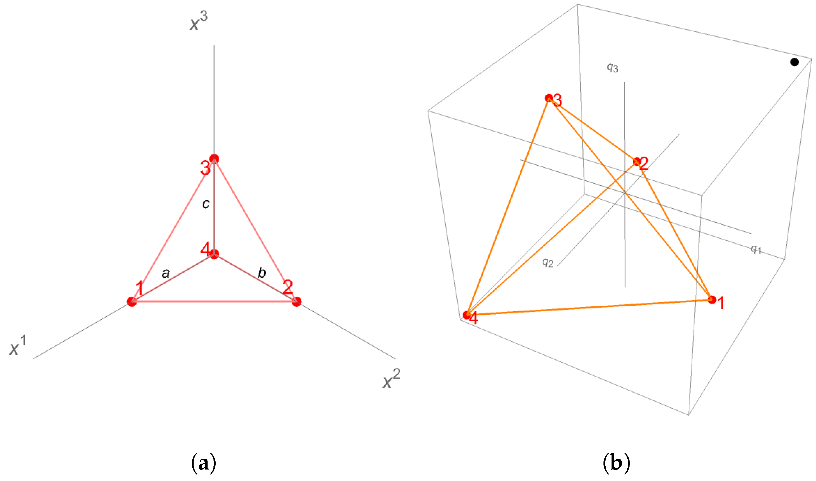
To illustrate the correspondence between the RPS and Bancroft’s solution, in this section, we use both approaches to solve the location problem for the case of four static emitters. This is a simple but clarifying example to gain insight into the RPS terminology. For any given time
t measured by an inertial observer of unit velocity
(
), we choose the simple spatial arrangement of an orthogonal tetrahedron as shown in
Figure 1a, where the reference emitter
is at the origin of the observer’s (spatial) coordinate system
.
The essential simplification that the static situation provides is the possibility to synchronise the emitters’ clocks at a given common (initial) instant. The respective proper times then become synchronised forever, which allows the representation of the static case in three-dimensional diagrams. We will come back to this point in
Section 8.
7.1. Emitters’ World-Lines and Emission/Reception Conditions
As the emitters’ clocks are synchronised at
taking
, the emitters’ world-lines, expressed with respect to an inertial reference frame
, can be easily written down in the case of static emitters:
where
are the position vectors of the other three emitters with respect to the fourth emitter:
where
are real constants, and where we have switched to component notation, with the first component being the coordinate time
. We can now write the position vector of the referred emitters with respect to the reference emitter:
where
. Then, substituting (
53) into (
11), we obtain the covariant components of the configuration vector
:
where
The Cartesian product
is included in the grid
of the positioning system and will be called the
-grid (quotient grid) according to the meaning of the triads
given below.
Figure 1b shows the emitters’ arrangement in the
-grid (see Equations (
76) and (
77)).
According to (
9), the emission/reception conditions are written as
and the emission condition is written as
with
given by (
17) in terms of
and
.
7.2. Computing the RPS Quantities
To compute the particular solution
(
12), we begin by setting
:
To obtain
, we calculate the world-function scalars
from (
53):
and the bivectors
from (
14), substituting (
53):
Computing the contractions
using (
3):
yields the covariant components of the particular solution
from (
12)–(
14) using (
57) and (
58):
To obtain the user’s inertial coordinates from (
16), we need the following to calculate
from (
17):
as follows from (
54) and (
60). Then, by substitution in (
18),
Notice that
is an even symmetric function,
, which is symmetric about the origin. With these quantities, we can express the coordinate transformation
using (
16)–(
18).
7.3. Interpretation of the RPS Solution
In order to remark on the essential properties of the RPS solution, let us consider the inertial coordinate locations of those users whose emission coordinates satisfy the restrictions
and
. Then, expressions (
60)–(
64) simplify, and their substitution into (
16) gives:
with
: that is,
, and
where
Then (
65) will be an emission solution iff, in addition to (
55) and
, Equation (
56) holds, with
given by (
66): that is,
Table 2 shows the result assuming
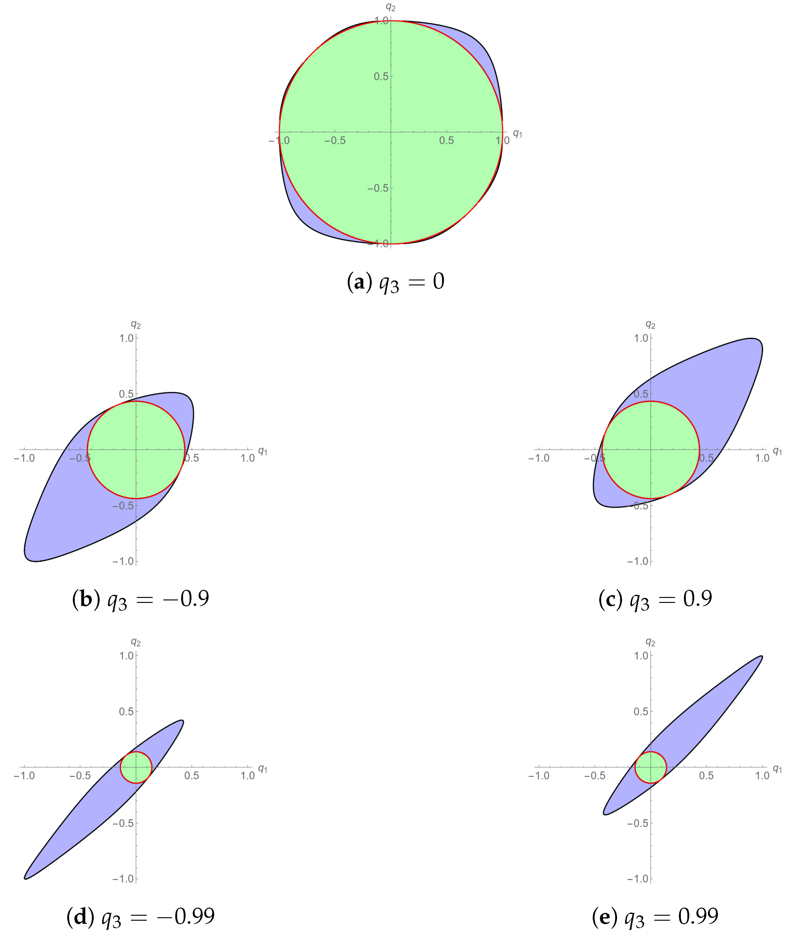
for different values of
q, where for the sake of clarity, we have taken
, and thus,
.
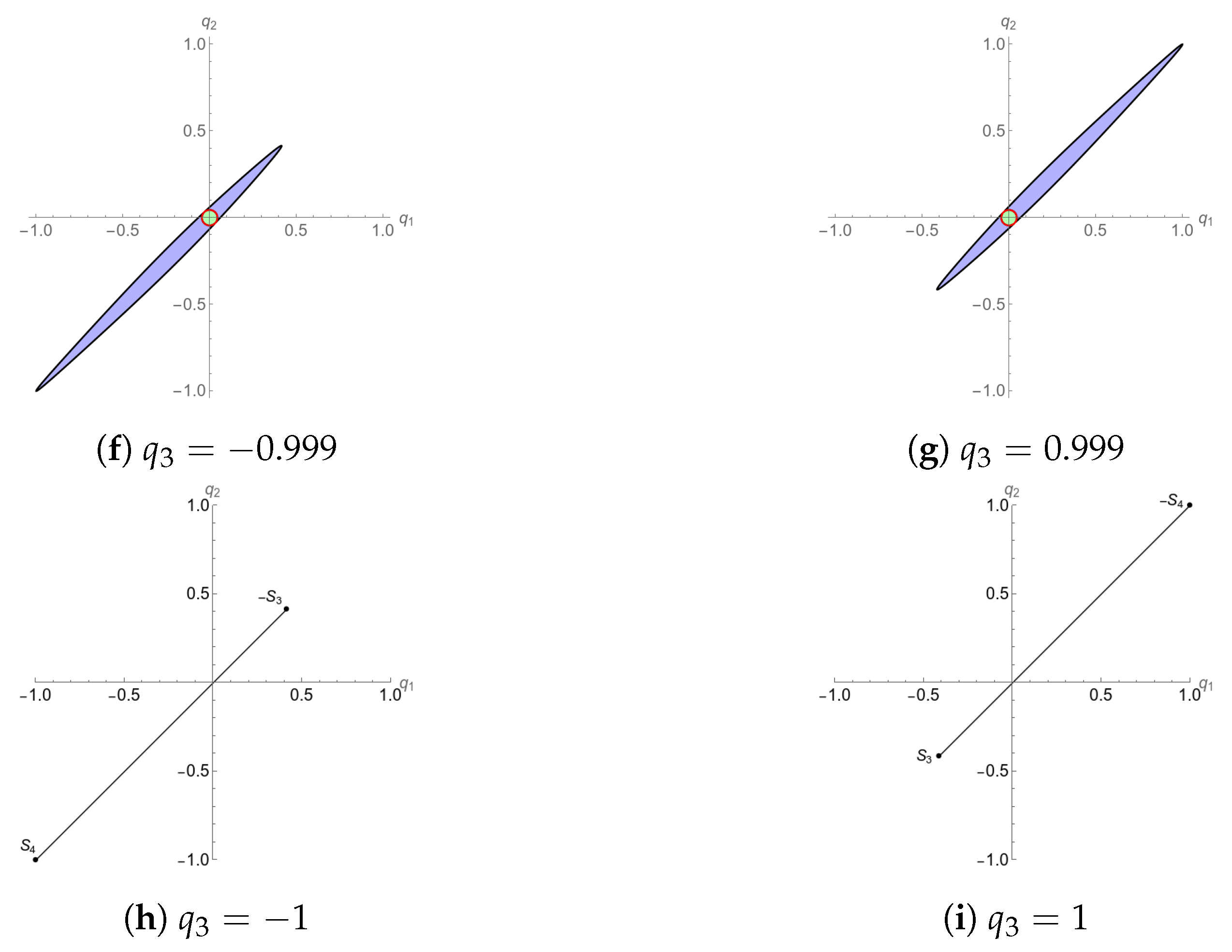
- (i)
For , the emitter configuration is space-like at , which is the sole emission solution (with ). The solution with is a reception solution.
- (ii)
For , the emitter configuration is light-like at , which is the sole emission solution (with ). The solution with is degenerate.
- (iii)
For
, the emitter configuration is time-like at
both being emission solutions (with
);
is in the front (back) emission coordinate domain.
Similarly,
Table 3 shows the result assuming
and
for different values of
q, where we have taken
, and thus
.
7.4. Computing Bancroft’s Quantities
In order to relate the RPS and Bancroft’s expression of the solution to the location problem, we begin by writing the matrix
given by (
25), for which the columns are the emitters’ world-lines (
51):
In component notation, we have:
To calculate
, we verify that:
and that the row vectors (1-forms)
appearing in (
33) and given by (
34) are expressed as:
where
is the dual basis of the inertial Cartesian basis.
Now we can write
as:
and then we compute the vector
u and verify (
41):
The vector
v is obtained from (
40) by substitution of (
70), (
71) and (
24) with
After simplification, the result is:
We can substitute (
73)–(
75) and
in Equation (
42) and check that it is satisfied.
To compute the user’s coordinates from Bancroft’s solution (
26) with
as in (
31) or (
32), we need the following expressions for
E,
F and
G, which follow from (
73) and (
75) by the scalar product:
Notice that Bancroft’s quantities E, F and G involve the emission coordinates in addition to . In contrast, the RPS quantities and are polynomial functions only of the variables. This property simplifies the representation of the RPS regions in the -grid, which is carried out in the next section.
9. Emission–Reception Conditions and Grid Regions
Figure 1b,
Figure 4 and
Figure 5 provide representations in the
-grid of the standard positioning data and the elements derived from these data. In this section, we use the
-grid representations to obtain further information about other regions where solutions to the null propagation Equation (
1) exist without imposing all of the emission/reception conditions (
55). We analyse a mixture of emission and reception conditions that apply to other location systems [
1,
2] based on null coordinates, such as reception or radar coordinates. For an analysis of the notion of a location system (physical realization of a coordinate system), see [
9] and previous references quoted herein.
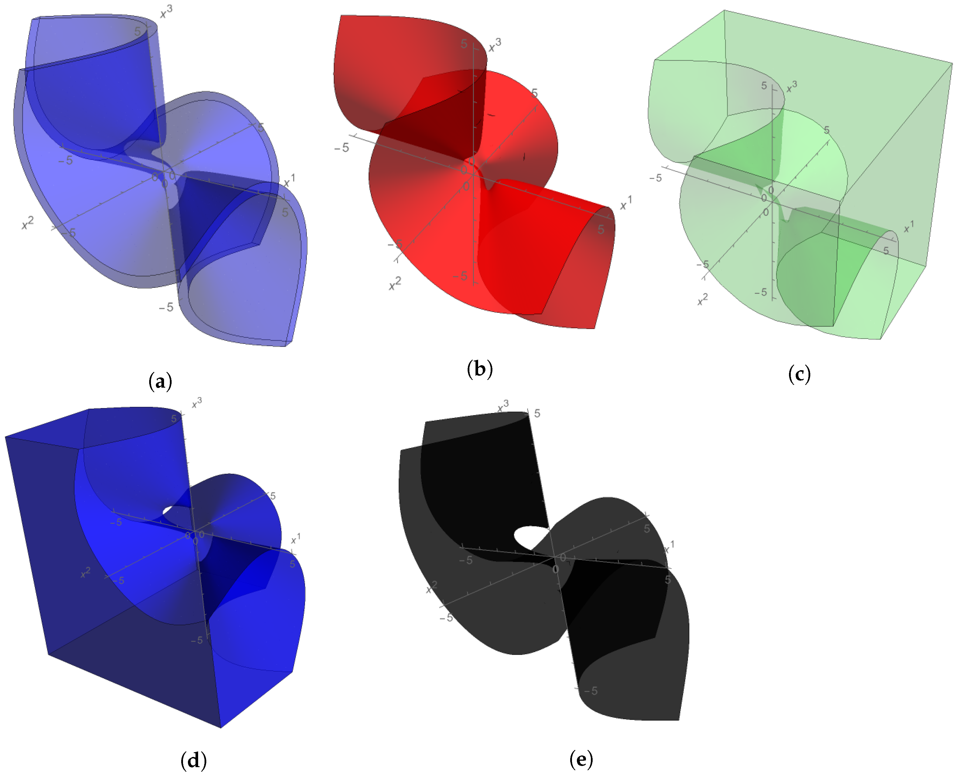
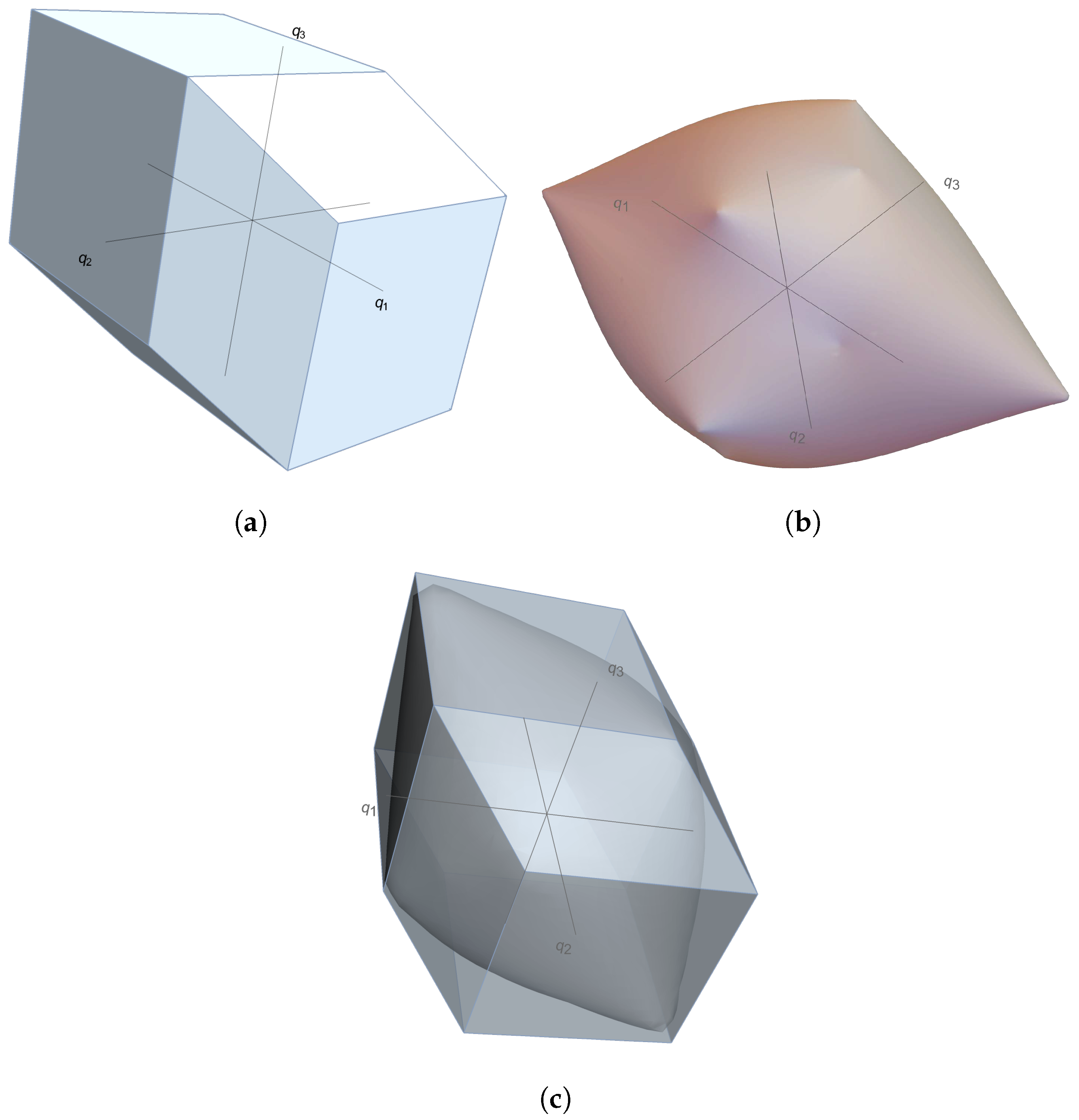
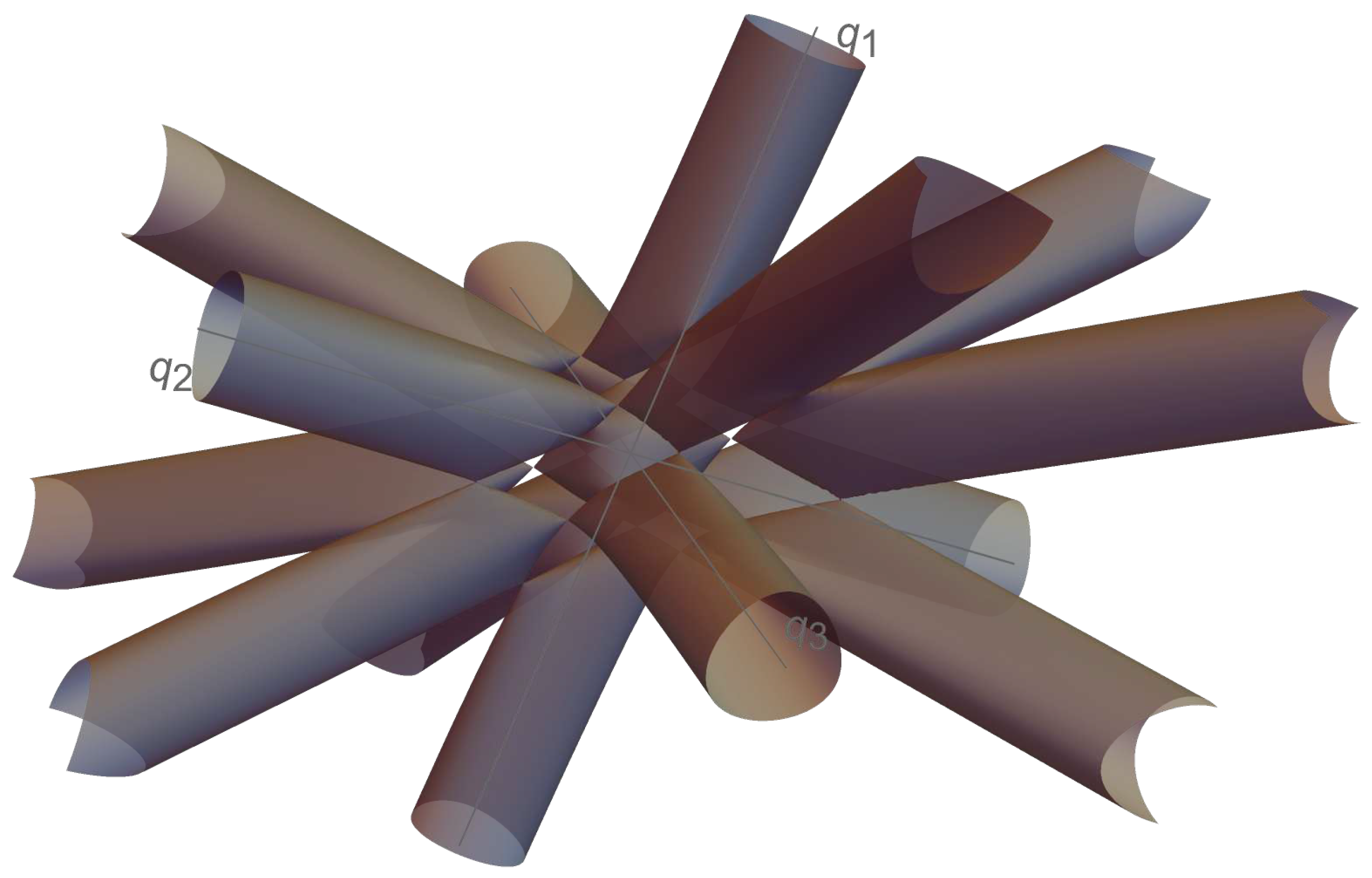
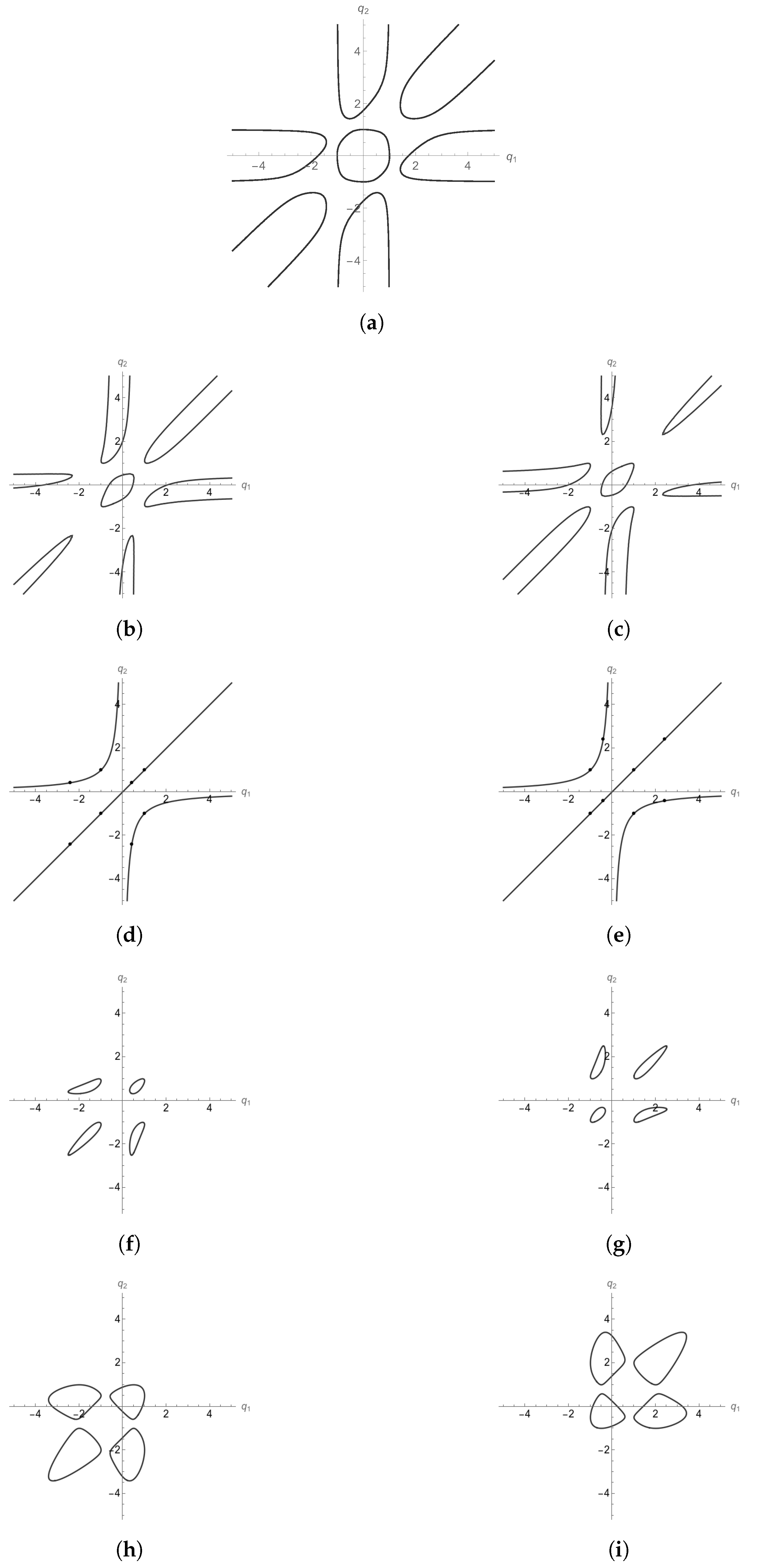
Figure 6 shows the surfaces in the
-grid defined by
, in whose interior there is a solution to the null propagation equations. There exist fifteen disjoint regions satisfying
. The exterior of this surface (
) has no physical meaning. The interior (
) is the
-grid representation of the solutions to the null propagation equations and is disjointly divided into fifteen regions. Only one region contains the origin, and it is divided in two subregions where all the emission/reception conditions are satisfied (see
Figure 4). Among the fourteen remaining regions, eight satisfy only three emission/reception conditions (each one is confined by three pairs of parallel planes). The other six satisfy only two emission/reception conditions (each one is confined by two pairs of parallel planes).
Table 4 shows the signs of the products
(
) and the related regions. The emission or reception character of a
-coordinate is denoted by
e or
r, respectively.
The results of this section may be compared with those presented in [
10,
11] regarding the 2D localization of a source with three receivers. In particular, there is an interesting similarity between the surface of the vanishing Jacobian (
Figure 6) and the Kummer surface represented in Figure 4 of [
11]. The surface shown in
Figure 6 has a total of thirty-two singular points—eight of them on the central piece and twenty-four on the tube-like pieces—with each of these points connecting the different pieces that make up the surface. In addition to
and
, the surface has the following singular points:
and their opposites. Of these singular points, only
and
are also vertices of
.
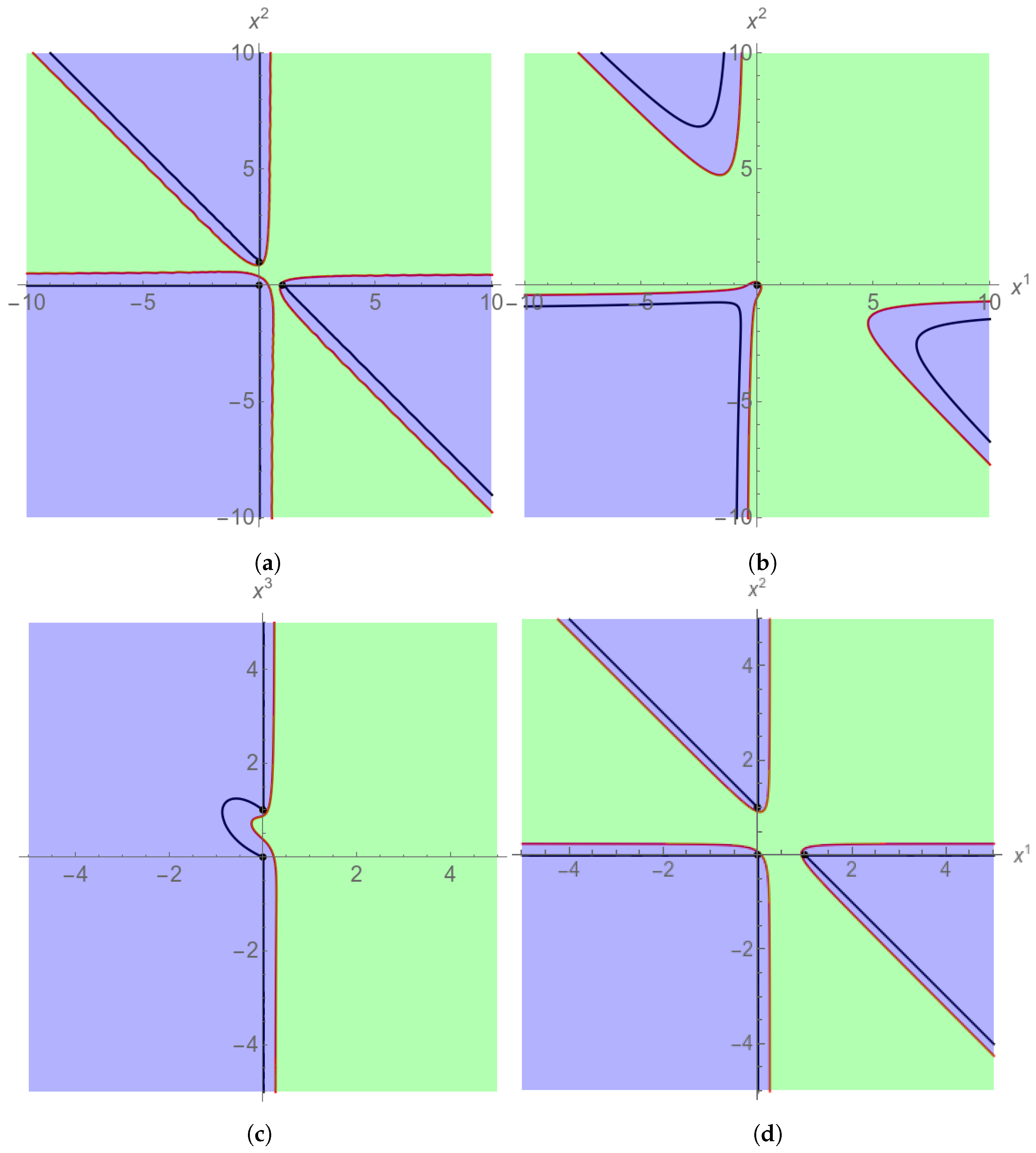
Figure 7 shows the cuts of the surface
with the different planes
. Similar cuts are obtained for constant values of
or
.
10. Conclusions
The RPS approach to GNSSs is grounded in the fundamental principles of relativity, on which, one might think, navigation systems should be based. Current GNSSs rely on a posteriori corrections for (special) relativistic effects (and for gravitational, atmospheric and instrumental effects). In this paper, we have deduced a classical solution to the navigation equations—Bancroft’s solution, which is still in use today—within a relativistic framework. In fact, Bancroft’s closed-form solution is suitable for this purpose since it already incorporates four-vectors and a Minkowski scalar product, although it still presumes a universal time and a deviation from it (the clock offset). We have recovered Bancroft’s solution from the RPS solution using the language of relativity: contravariant (column) and covariant (row) vectors, their inner (scalar) product and their exterior algebra.
The characteristic elements of an RPS (emission and configuration regions, front and back coordinate domains, shadows produced by the satellites to each other, etc.) have been exemplified for the static situation. These regions are represented both in the physical and in the grid space of the RPS by introducing an appropriate quotienting procedure. This kind of representation has been tentatively studied for other location systems for which not all the emission/reception conditions are assumed. However, to deal with general location systems, the RPS terminology should be appropriately adapted.
All of this is with the hope of bringing the traditional GNSS approach closer to the framework of Relativity Theory: a worthwhile task, if only from a scientific perspective.


