Small-Scale Cosmology Independent of the Standard Model

Abstract

‘Small-scale cosmology’ is a theory designed to incorporate the linear redshift versus distance relation, which is inferred from observations, into the theoretical framework independent of the global Robertson–Walker–Friedman (RWF)-type models. The motivation behind this is that the RWF cosmological models, based on the assumptions of homogeneity and a constant matter density, as well as the concept of expanding space inherent to them are not applicable on the scales of observations from which the linear Hubble law is inferred. Therefore, explaining the Hubble law as the small redshift limit of the RWF model or as an effect of expanding space is inconsistent. Thus, the Hubble linear relation between the redshift of an extragalactic object and its distance should be considered an independent law of nature valid in the range of the distances where the RWF cosmology is not valid. In general, the theory, based on that concept, can be developed in different ways. In the present paper, ‘small-scale cosmology’ is formulated as a theory operating in the (redshift–object coordinates) space, which allows developing a conceptual and computational basis of the theory along the lines of that of special relativity. In such a theory, the condition of invariance of the Hubble law with respect to a change in the observer acceleration plays a central role. In pursuing this approach, the effectiveness of group theoretical methods is exploited. Applying the Lie group method yields transformations of the variables (the redshift and space coordinates of a cosmological object) between the reference frames of the accelerated observers. In this paper, the transformations are applied to studying the effects of the solar system observer acceleration on the observed shape, distribution and rotation curves of galaxy clusters.

1. Introduction

Modern cosmology started with Hubble’s discovery of the linear redshift–apparent magnitude relation for nearby galaxies. Soon after the discovery, it was interpreted as direct observational evidence for an expanding universe, meaning that it agrees with the expanding solution of Einstein’s equations (more specifically the Friedman equation). Although, at that stage, the general relativity (GR) was engaged to interpret the discovery. In fact, the symmetry, expressed by the Robertson–Walker (RW) metric (see, for example, [1,2]) and based on the assumptions of homogeneity and isotropy of the universe, is sufficient. It provides the interpretation of Hubble’s Law as a consequence of the RW symmetry for small redshifts illustrated by the linear region in the luminosity distance versus the redshift curve. The dynamics based on the GR equations, which are reduced to the Friedman equations under the assumption of a constant density, are needed for defining the expansion parameters, particularly cosmological acceleration.

The issue of acceleration emerged much more recently, being announced by Perlmutter, Riess and their colleagues [3,4] as the result of work using supernovae of Type Ia as standard candles. The Hubble law played a significant role in that work. The point is that SNe Ia are not really standard candles. If they all were of the same maximum luminosity, then they would be ideal for standard candles owing to their high luminosity, which allows them to be detected even at large distances. However, the SNe Ia maximum luminosity varies from object to object, as was revealed by the Hubble diagram for relatively nearby SNe Ia. Belief in validity of the Hubble law for nearby objects was a crucial point for the analysis, as it was presumed that, in the case of all SNe Ia having the same maximum luminosity, the data points in the diagram should be aligned along a straight line, as follows from the Hubble law. However, a scatter around the Hubble relation was significantly larger than the photometric measurement errors.

Two advancements allowed overcoming this challenge. First, Phillips [5] found convincing evidence for a correlation between the light curve shape and the luminosity at maximum brightness. Namely, the slower the decline, the higher the absolute luminosity. Next, it was understood that the observed flux is possibly affected by extinction in the host galaxy, in addition to extinction in the Milky Way. The colors of SNe Ia provide a way to correct for extinction with dust in both our galaxy and the host. The combined analysis of these effects gives a possibility for deducing an empirical correction to the maximum luminosity, accounting for both the relation of the decline and width of the light curve to the observed luminosity and for the extinction. The Hubble diagram for nearby SNe Ia, plotted with the corrected data, was commonly used as a consistency test for a method of parametrization of the effects (e.g., [6,7,8,9,10]). It was found that with a proper ‘standardization’ of the luminosity, the deviations from the Hubble law became dramatically smaller. As a result, SNe Ia indeed became standard candles, providing quite accurate relative distances.

All of the above shows that in the cosmic acceleration discovery, the validity of the Hubble law for cosmologically nearby objects played a significant role, providing both a crucial test and strong support for using the corrected SNe Ia observational data as relative distance indicators. The belief in the validity of the Hubble law for the objects at small redshifts z is usually justified by the luminosity distance $d_L$ versus the redshift z’s curve, obtained either as a kinematical consequence of the RW metric or as a solution to the Friedman equation of GR, being approximately linear in the small z part. However, it is important to remember that the assumptions of homogeneity and a uniform density underlying the Robertson–Walker–Friedman (RWF) cosmological model are supported by the observational evidence only after averaging the observed universe over scales that are many orders of magnitude larger than those on which the calibration of the SNe Ia data were implemented. The objects of our local universe are filtered out as a result of such averaging, and only then does the distant universe look approximately uniform or homogeneous. Observations of the distribution of galaxies in our local universe clearly show that the assumptions of homogeneity and a constant density become meaningless at those scales. Therefore, claiming the Hubble law to be the small z limit of the luminosity distance versus the redshift curve, obtained within the framework of the Robertson–Walker–Friedman (RWF) cosmology, is an inconsistent application of the model on scales where the assumptions, and thus the results, of the model are invalid. In a sense, this is similar to applying the continuum equations (Euler or Navier-–Stokes) to rarefied gas, where the molecular mean free path is not negligible.

Another widespread interpretation of the Hubble law, as an effect of expanding space, is somewhat related to the above discussion. This interpretation emerged soon after the Hubble 1929 discovery, when the Hubble observations were set within the framework of general relativity or, more precisely, the GR-based Robertson–Walker–Friedman cosmology. It is clear from the FRW form of the spacetime metric that for a fixed coordinate of time t, the physical separation of objects depends on the size of the scale factor $a\left(t\right)$, and the increase in $a\left(t\right)$ with t results in the increasing separation of objects. This is typically taken to be the expansion of space. Usually, in textbooks, when the expanded space concept is introduced, space is represented as being defined by a network of comoving coordinates and analogies of stretching rubber sheets or a river, carrying matter along with it in its motion. As was formulated in [11], ‘According to the expanding space paradigm … the galaxies do not move through space, but instead float stationary in space. Their separating distances increase because the space between the galaxies expands’.

The concept of expanding space has been the subject of considerable debate, and explaining the increasing separation of galaxies with the expansion of space has recently been criticized from different points of view (e.g., [11,12,13,14,15,16]) as an idea which leads to confusion and misconceptions. J.A. Peacock [13] stated that ‘… the very idea that the motion of distant galaxies could affect local dynamics is profoundly anti-relativistic …’ A.B. Whiting [12] claimed the following: ‘The fact that space in GR has an active role in dynamics, however, does not mean it has the attributes of a physical object. It does not act like a viscous fluid, drawing all bodies into the Hubble flow, even asymptotically; it does not affect things by ‘expanding’, nor by accelerating this expansion’. S. Weinberg, in the course of discussing the Big Bang issue in [17], answered the question:

Popular accounts, and even astronomers, talk about expanding space. But how is it possible for space, which is utterly empty, to expand? How can ‘nothing’ expand?

’Good question’, says Weinberg. ‘The answer is: space does not expand. Cosmologists sometimes talk about expanding space—but they should know better’.

It was found in [18] that the concept of the expansion of space could acquire meaning only in the context of mathematics of general relativity from which it arose. In the FRW cosmological model, the dynamics of the expansion is defined by solving the GR field equations under the assumptions that a homogeneous universe is filled with a fluid of uniform density and that the test observers can measure their velocity with respect to that fluid. The privileged observers, whose watches are synchronized with cosmic time, are at rest with regard to the cosmic fluid, and the change in the metric with time via the scale factor implies that (in an expanding universe) the physical distance between any two privileged observers increases with time. Thus, only under the assumption of a homogeneous universe filled with a fluid of a uniform density does ‘the expansion of space’ acquire the meaning of an increase in the distances between privileged observers that are at rest with respect to that fluid. The same is stated in [12]: ‘In fact, if one looks at space itself apart from the associated fluid of cosmological matter, it is not at all certain what ‘the expansion of space’ means’. The concept of cosmic homogeneous fluid filling all the space, which is inherent in the RWF cosmological model, is evidently not valid on the scales of galaxies. This was concluded in [18]: ‘The expansion of space is global but not universal, since we know the FRW metric is only a large scale approximation’, and ‘… we should not expect the global behaviour of a perfectly homogeneous and isotropic model to be applicable when these conditions are not even approximately met. The expansion of space fails to have a ‘meaningful local counterpart’.

Thus, validity of the linear Hubble law at cosmologically small scales cannot be proven within the framework of the standard model based on the global RWF spacetime. Nevertheless, the low-redshift SNe Ia data, corrected according their pick luminosity (e.g., [7,8,9,10]), provide the best evidence that the relation between the distance modulus and redshift of an object is linear. Thus, validity of the Hubble Law at cosmologically small scales should be admitted despite the fact that, at those scales, it cannot be explained with reference to the RWF-type models or by the expansion of space. This suggests that we have to accept the Hubble linear relation between the redshift of an extragalactic object and its distance as a physical reality which may be considered a law of nature and, as such, used as the basis for the theory.

The theory, based on the above statement, could be questioned on the grounds that gravity, which is a ubiquitous phenomenon, is not involved in the framework. We note in this respect that, in fact, the modern cosmology is built of two parts such that the primary part, cosmography, does not involve any issues related to gravity but serves as a basis for the second part, which applies GR to the analysis of the observational data. Cosmography analyzes the observations based on the cosmological principle (Copernican principle), which implies validity of the assumptions of spatial homogeneity and isotropy and leads to the Robertson–Walker metric in that way. Then, astronomical observations can be interpreted as measurements of the scale factor $a\left(t\right)$ and the curvature constant k. In particular, the RW metric can be used to derive the luminosity distance $d_L$ versus the redshift z relation as a power series:

$$d_L=H_0^{-1}\left(z+\frac{1}{2}\left(1-q_0\right)z^2+\cdots \right)$$

(1)

where $H_0$ is endowed with the meaning of the Hubble constant, and with the interpretation of the redshift as a recession velocity, $q_0$ acquires the meaning of the ‘deceleration parameter’ of the cosmological expansion. The dynamics of the cosmological expansion is treated by applying the gravitational field equations of Einstein which, upon making some tentative assumptions about the constituents of the universe and their properties, allows one to relate the parameters of the expansion contained in Equation (1) to the values of the cosmic energy density and pressure.

The above outlined framework of the large-scale cosmology was seriously challenged by the SNe Ia data which correspond to the deceleration parameter $q_0<0$. (The expansion of the universe is accelerating.) This result contradicts the results of applying the matter-dominated cosmological model of the universe which yields the luminosity distance–redshift relation with the deceleration parameter $q_0$, which is positive for all three possible values of the curvature parameter k. This stimulated an avalanche of explanations, with many involving speculative new physics. In the modern cosmology, represented by the standard $\mathsf{\Lambda }$CDM model, that challenge is resolved by introducing dark energy, a new component of the energy density with strongly negative pressure that makes the universe accelerate. The challenge caused by the SNe Ia data did not touch the cosmography part of the description of the large-scale universe since that part is not influenced by changes in the view on the constituents of the universe, modifications to the field equations or the introduction of alternative theories of gravity.

The approach adopted in the present study may be identified as the small-scale cosmography since, like the large-scale cosmography, it does not refer to any physics in justifying the basic assumptions of the theory but nevertheless provides a theoretical framework for interpretation of observations. The meanings for the terms ‘large-scale’ and ‘small-scale’ are provided by the scales of validness of the basic assumptions of the theories. In the large-scale cosmology, it is the homogeneity scale, and in the small-scale cosmology, it is the scale in which the linear Hubble law is valid. Both scales cannot be precisely determined. In particular, the homogeneity scale ‘depends on the averaging procedure (see, for example, the discussons in [19,20,21,22]). A.A. Coley and G.F.R. Ellis in their review of theoretical cosmology [23] remarked that ‘… it would thus be better if the cosmological principle could be deduced rather than assumed a priori (i.e., could late time spatial homogeneity and isotropy be derived as a dynamical consequence of the Einstein field equations (EFE) under suitable physical conditions and for appropriate initial data)’. This statement of Colley and Ellis regarding the potential role of gravity in the large-scale cosmography is completely applicable to the discussion of the (potential) role of gravity in the present framework. If the Hubble law could be deduced from the GR equations as the solution of the many-body problem of interacting galaxies, then this would provide a physical background for the theory, but this is an intractable task.

When presenting a cosmological model, it is unavoidable to discuss the (potential) role in the theory of the two issues inherent to the modern cosmology: dark matter and dark energy. Starting with dark matter, we remark that, in fact, dark matter arises in two conceptually different contexts. The first one is related to cosmologicaly small scales, where dark matter is introduced to explain some gravitational effects that cannot be explained within the framework of general relativity unless more matter is present than can be seen. Such effects occur in the galaxy rotation curves, the motion of galaxies within galaxy clusters, gravitational lensing, mass position in galactic collisions and some other instances (see, for example, [24,25,26]). Dark matter, as a substance whose presence is discerned from its gravitational attraction rather than its luminosity, is not known to interact with ordinary baryonic matter and radiation except through gravity, making it difficult to detect in a laboratory. The most prevalent explanations of its nature range from some (not-yet-discovered) particles, like weakly interacting massive particles (WIMPs) or axions, to primordial black holes (see, for example, [27,28,29]).

While the hypothesis of dark matter in the above discussed context has an elaborate history, rising to ‘missing mass’ in galaxy clusters, as inferred by Fritz Zwicky in 1933, the concept of dark matter in the second context, related to large-scale cosmological models, arose only in the early 1990s after discovering the accelerated expansion of the universe. In that context, dark matter is one of the energy components in the stress tensor of the general relativity equation. In the standard model of cosmology, the dynamics of the expansion is governed by the general relativity equations that reduce to the fundamental Friedman equation, defining the time dependence of the scale factor $a\left(t\right)$ as follows (see, for example, [2]):

$$a^{\prime 2}\left(t\right)=-K+\frac{8\pi G}{3}{a}^2\left(t\right)\rho \left(t\right)$$

(2)

where G is Newton’s gravitational constant and K is the curvature parameter. Applying this equation requires making assumptions about the constituents of the cosmic energy density $\rho$. It is assumed to be a mixture of non-relativistic matter, which means any constituent of the universe whose energy density scales with the inverse cube of the scale factor (i.e., ${\rho }_M\sim a^{-3}$), the relativistic matter (radiation), which scales as the inverse fourth power of the scale factor ${\rho }_R\sim a^{-4}$, and dark energy (usually named the vacuum energy), which does not change with a (i.e., ${\rho }_V\sim a_0$), which is equivalent to introducing into Einstein’s equation a cosmological constant $\mathsf{\Lambda }$. Thus, $\rho \left(t\right)$ is expressed as

$$\rho \left(t\right)=\frac{3H_0^2}{8\pi G}\left({\mathsf{\Omega }}_{\mathsf{\Lambda }}+{\mathsf{\Omega }}_{M}x{\left(t\right)}^{-3}+{\mathsf{\Omega }}_{R}x{\left(t\right)}^{-4}\right)$$

(3)

where

$$x\left(t\right)=\frac{a\left(t\right)}{a_0},a_0=a\left(t_0\right)$$

(4)

The parameters ${\mathsf{\Omega }}_{\mathsf{\Lambda }}$, ${\mathsf{\Omega }}_M$ and ${\mathsf{\Omega }}_R$ are defined by

$${\mathsf{\Omega }}_{\mathsf{\Lambda }}=\frac{{\rho }_{V0}}{{\rho }_c},{\mathsf{\Omega }}_M=\frac{{\rho }_{M0}}{{\rho }_c};{\mathsf{\Omega }}_R=\frac{{\rho }_{R0}}{{\rho }_c};{\rho }_c=\frac{3H_0^2}{8\pi G}$$

(5)

where ${\rho }_{V0}$, ${\rho }_{M0}$ and ${\rho }_{R0}$ are the present values of the densities and ${\rho }_c$ is the critical energy density. The components of the energy density satisfy the following equation (a consequence of Equation (2) evaluated at $t=t_0$):

$${\mathsf{\Omega }}_{\mathsf{\Lambda }}+{\mathsf{\Omega }}_M+{\mathsf{\Omega }}_R+{\mathsf{\Omega }}_K=1;{\mathsf{\Omega }}_K=-\frac{K}{a_0^2{H}_0^2}$$

(6)

It is found that the radiation density parameter ${\mathsf{\Omega }}_R$ is negligible compared with other $\mathsf{\Omega }$ values. The values of the parameters ${\mathsf{\Omega }}_{\mathsf{\Lambda }}$, ${\mathsf{\Omega }}_M$ and ${\mathsf{\Omega }}_K$ are defined by fitting the $d_L\left(z\right)$ (luminocity distance – redshift) dependence retrieved from the SNIa observational data into that derived from the solutions to the Friedman equation. First of all, it is found that for ${\mathsf{\Omega }}_{\mathsf{\Lambda }}=0$ (i.e., without introducing dark energy), fitting is impossible. In this case, the solutions of the Friedman equation correspond to decelerating expansion for any value of the curvature parameter. In the case of ${\mathsf{\Omega }}_{\mathsf{\Lambda }}\ne 0$, the best fitting is achieved with ${\mathsf{\Omega }}_K=0$, (The universe is flat, which is supported by other observations.) ${\mathsf{\Omega }}_M\approx 0.3$ and ${\mathsf{\Omega }}_{\mathsf{\Lambda }}\approx 0.7$. In this fitting, ${\mathsf{\Omega }}_M$ corresponds to any substance evolving with time as $a^{-3}$, particularly the ordinary, visible matter. The amount of visible matter in the universe can be estimated, and the estimation is that it constitutes only five percent of the mass–energy content, and the rest is ‘dark matter’. Thus, in this context, dark matter makes an appearance as a component of a cosmic fluid which, together with dark energy, uniformly fills the space in the large-scale averaged RWF model. It is evident that this component of the cosmic fluid of the large-scale $\mathsf{\Lambda }$CDM model should not be identified with the invisible gravitating substance introduced to make the small-scale astrophysical models consistent with general relativity. The density of dark matter as a component of cosmic fluid is tied to the density of dark energy by the requirement of fitting the SNIa data, and therefore it is not clear at all that the artificially introduced substance is of the same nature as the invisible matter in galaxies and clusters.

When discussing the relevance of dark matter to the ‘small-scale cosmology’ developed in the present paper, one should distinguish between the two contexts in which the concept is involved. Regarding the potential role of dark matter, as an invisible matter in galaxies and galaxy clusters, we can state again the following: if the Hubble law could be deduced from the GR equations as the solution of the many-body problem of interacting galaxies, then of course the input of invisible but gravitating matter should be accounted for. However, since this is impossible, dark matter in this context plays no role in the framework of the present cosmographycal model of a small-scale cosmology. Regarding the second large-scale context of dark matter’s emergence, we can repeat what was said above in the discussions of applicability of the results of the RWF model to small scales: the FR metric is only a large-scale approximation, and the basic assumptions of the RWF model, homogeneous and isotropic space and the uniform-density cosmic fluid filling it are not expected to be applicable when these conditions are not even approximately met.

Dark energy, distinct from dark matter, came to light only at the beginning of the 1990s as the dominant contribution to the energy content needed to provide fitting of the distance–redshift relation obtained from the RWF model to one retrieved from the SNIa observations. Later dark energy, as a (main) part of the conceptual framework of the standard $\mathsf{\Lambda }$CDM model of cosmology, had been used for interpretation of some other observational facts, particularly the flatness of the universe and large-scale wave patterns of mass density in the universe. The nature of dark energy remains a mystery, and explanations abound. The most popular explanation, vacuum energy, (The term ‘vacuum energy’ is commonly used as an equivalent of ‘dark energy’.) should be considered inappropriate because of the substantial disagreement between the observed values of the vacuum energy density and the much larger theoretical value of the zero-point energy suggested by quantum field theory. The ‘cosmological constant’, as a source term that can be added to Einstein field equations of general relativity, is commonly viewed as equivalent to ‘vacuum energy’. The cosmological constant interpretation does not resolve a huge disagreement between the values observed and deduced from quantum field theory for the vacuum energy density, and the problem appears in the literature under two names: the ‘cosmological constant problem’ or ’vacuum catastrophe’. It should also be mentioned that sometimes, dark energy is identified with a negative pressure field which could drive cosmic inflation in the extremely early universe. However, inflation must have occurred at a much higher (negative) energy density than in the dark energy we observe today, and thus it is doubtful that there exists any relation between dark energy and inflation.

It is evident from the above that dark energy is a concept inherent only to the large-scale RWF cosmological model in which, upon large-scale averaging, a homogeneous universe is filled with a fluid of a uniform density, with dark energy being one of the components. Nevertheless, there is a tendency to extend the concept to small scales, treating dark energy as a smooth, persistent component of invisible energy filling (otherwise empty) space and not accumulating preferentially in galaxies and clusters, and applying the $\mathsf{\Lambda }$CDM model to explaining the processes on the scales of galaxies and clusters. Note that many observations on galaxy scales now seem to be in conflict with the $\mathsf{\Lambda }$CDM paradigm, such as the overabundance of the predicted number of halo substructures, compared with the observed number of satellite galaxies and the discrepancy between the measured densities at the halflight radii of the brightest local dwarf galaxies and the (higher) densities of the most massive subhalos in $\mathsf{\Lambda }$CDM simulations (see, for example, [30,31,32,33]). Curious discrepancies also appear to exist between the predicted clustering properties of CDM on small scales and observations (see, for example, [34] and the references therein). However, independent of those issues, it should be stated that extending the notion of dark energy, related to the global large-scale dynamics of the universe, to small scales is conceptually inconsistent. Thus, dark energy is irrelevant to the small-scale cosmological model developed in the present paper.

In general, the $\mathsf{\Lambda }$CDM model has been proven to be explanatory and even predictive, providing us with substantial understanding of observations on large scales. Nevertheless, it is a heuristic theory, which explains the observational data without being able to provide a theoretical foundation for its basic assumptions. The nature of dark energy (treated either as vacuum energy or the cosmological constant) as well as the particle nature of dark matter are entirely mysterious. This and other unresolved serious theoretical issues motivate developing alternative theories, such as the modified gravity theories and the varying fundamental constant theories. Thus far, none of the proposed theories can successfully describe every piece of observational data, which are usually considered as supporting the $\mathsf{\Lambda }$CDM model, at the same time.

In this context, it is worthwhile to draw attention to ‘relativity with a preferred frame’ [35], which provides the possibility of explaining the main body of the observational data, commonly mentioned in support of the $\mathsf{\Lambda }$CDM model, within the framework of the RWF cosmology but without introducing dark energy and dark matter. Distinct from other theories extending cosmology beyond the standard model, in ‘relativity with a preferred frame’, no ad hoc assumptions are made, the fundamental laws of physics do not change, and relativistic invariance is not violated. It is also important that the theory is designed without any relations to possible applications. Modifications, ingrained into the theory at the fundamental level of special relativity, are introduced to reconcile the existence of the cosmological preferred frame (usually identified with the CMB frame) with the relativity principle. The postulates of special relativity, namely the relativity principle and universality of the speed of light, are retained. Only the freedom in the value of the one-way speed of light is used such that there is an anisotropy of the one-way speed of light in all the frames except for the preferred frame, while the two-way speed of light is equal to c in all of the frames. This does not spoil relativistic invariance and does not change the form of physical laws. The preferred fame effects reveal themselves only in that the time and space intervals figuring into equations expressing physical laws should be transformed into ’physical’ (measurable) intervals using some relations in which only one parameter, the anisotropy parameter b, figures in. This results in particular in the expression for the redshift containing some coefficient dependent on b such that applying the arguments which led to the $d_L\left(z\right)$ relation in Equation (1) in the standard RW model yields a modified relation of the form

$$d_L=H_0^{-1}\left(z+\frac{1}{2}\left(1-q_0-b\right)z^2+\cdots \right)$$

(7)

The luminosity distance–redshift relation in Equation (7), in principle, makes it possible to fit the SNIa observations to the matter-dominated RWF model. According to Equation (7), the observed deceleration parameter is $q_0^{\left(obs\right)}=q_0+b$, with $q_0$ being the deceleration parameter of the RWF matter-dominated model. Since the parameter b is expected to be negative, the observed negative values of $q_0^{\left(obs\right)}$ do not exclude the Friedman dynamics with $q_0>0$, which implies that the universe can be both accelerating and decelerating. Although it is an indication of the SNIa data being explainable within the framework of the RWF model without introducing dark energy, in order to prove this, the Friedman equation (Equation (2)) is to be solved, and the $d_L\left(z\right)$ dependence derived from the solution is to be compared with that retrieved from the SNIa observations. Assuming, in contrast to the standard model, that in Equations (4) and (6), ${\mathsf{\Omega }}_{\mathsf{\Lambda }}=0$, one can find the solution to the Friedman equation containing only ${\mathsf{\Omega }}_M$ and b. (${\mathsf{\Omega }}_K$ can be eliminated using Equation (6).) By applying this solution, there is no need to specify the nature of the matter density characterized by ${\mathsf{\Omega }}_M$. It could either be only the ordinary matter or the mixture of ordinary and dark matter. In the latter case, however, there is a conceptual difference from the $\mathsf{\Lambda }$CDM standard model. While, in the standard model, dark matter is a component of the cosmic fluid whose density is tied to the dark energy and thus has no connection to the small-scale dark matter density, in the model, based on ‘relativity with a preferred frame’, it could be an average of the estimated density of dark matter (presumably) accumulated in galaxies and clusters. It was shown in [35] that for any value of ${\mathsf{\Omega }}_M$, the value of the model parameter b can be found such that the $d_L\left(z\right)$ dependence, derived using the solution, fits the SNIa data with high accuracy. (In fact, $d_L\left(z\right)$ of the $\mathsf{\Lambda }$CDM ‘concordance’ model was used as a fitting formula for the SNIa data.) The result is represented by a curve in the plane (${\mathsf{\Omega }}_M$, b) on which fitting is achieved.

The framework of ’relativity with a preferred frame’, designed from the level of the special relativity foundations, is not specified for any applications and thus can be applied for interpreting other observations within the same framework. The baryon acoustic oscillation (BAO) data are commonly considered as confirming the accelerated expansion and imposing constraints on the dark energy parameters. The BAO observations provide two different sets of data: BAO scales in the transverse and line-of-sight directions. Measurements of the angular distribution of galaxies yield the quantity $D_M\left(z\right)$, which is the comoving angular diameter distance. Measurements of the redshift distribution of galaxies yield the value of the Hubble parameter $H\left(z\right)$. In the results, obtained within the framework of ’relativity with a preferred frame’ and represented by the regions in the plane (${\mathsf{\Omega }}_M$, b), within which the predictions of the present theory fit the $D_M\left(z\right)$ and $H\left(z\right)$ data, the two regions are overlapped. This both provides a support for the theory and places quite tight constraints on the values of the parameters ${\mathsf{\Omega }}_M$ and b, which are confined within a quite narrow overlapping region. An additional (and quite strong) argument in favor of both consistency of the theory and the estimates for the parameter b is that the line in the plane (${\mathsf{\Omega }}_M$, b), on which the results of the model fit the SNIa data, lies within that narrow region. It deserves attention that the value of ${\mathsf{\Omega }}_M=1$, which in light of Equation (6) corresponds to the value ${\mathsf{\Omega }}_K=0$ (flat universe), is within the overlapping interval. Thus, the results fit three different sets of observational data well, with the values of the theory parameter b confined within a quite narrow interval.

Next, the observations of temperature anisotropies in the CMB are commonly considered as providing another independent test for the existence of dark energy. In the standard model, the presence of dark energy affects the CMB anisotropies, leading to a shift in the positions of the acoustic peaks. In the model, based on ’relativity with a preferred frame’, that change can be attributed to the presence of the correction factor in the relation for the redshift. What is more, ‘relativity with a preferred frame’ allows explaining the pussling Auger data on the mass composition of cosmic rays without introducing new physics [36], and it also explains some abnormal features in the gamma ray spectrum [37]. It is remarkable that only one universal parameter b figures into the theory and that the values of the parameter are within the same range in all cases. All of the above are the hallmarks of a good and valuable physical theory. Thus, ‘relativity with a preferred frame’, designed to reconcile the relativity principle with the existence of the cosmological preferred frame, may provide an alternative to the standard model of cosmology (at least in some aspects).

Returning to the theory developed in the present paper, it is worth emphasizing that although a cosmological model relying on the universality of the Hubble law may be challenged (as with any model), the conclusion that the local Hubble law cannot be explained in the framework of the currently accepted standard model of the large-scale cosmology and thus should be considered as an independent law of nature (within its area of validness) cannot be challenged. In this respect, it is appropriate to comment on the so-named ’Hubble tension’ which is currently a widely discussed issue. Hubble tension refers to a growing discrepancy between the Hubble constant value, inferred from early universe probes (observations of CMB anisotropies by Planck) assuming the standard flat $\mathsf{\Lambda }$CDM cosmological model [38], and the measurement of that value from late-universe probes by the SHOES project [39,40]. It is frequently suggested that the difference might be an indicator of new physics. However, in light of the above discussion, the Hubble tension does not exist. There are no grounds to identify the value of the Hubble constant in the Hubble law, inferred from the measurements in the local universe, with the constant $H_0$ in the $d_L\left(z\right)$ relation in Equation (1) obtained from the highly smoothed and symmetrized RW cosmological model. Although in the discussions of the Hubble tension in the literature, both values are referred to as the ‘current expansion rate of the universe’, they are related to different conceptual frameworks. The term ‘expansion’ implies the RWF model which, like as the term itself, is not applicable to the interpretation of local observations. Therefore, no coincidence should be expected.

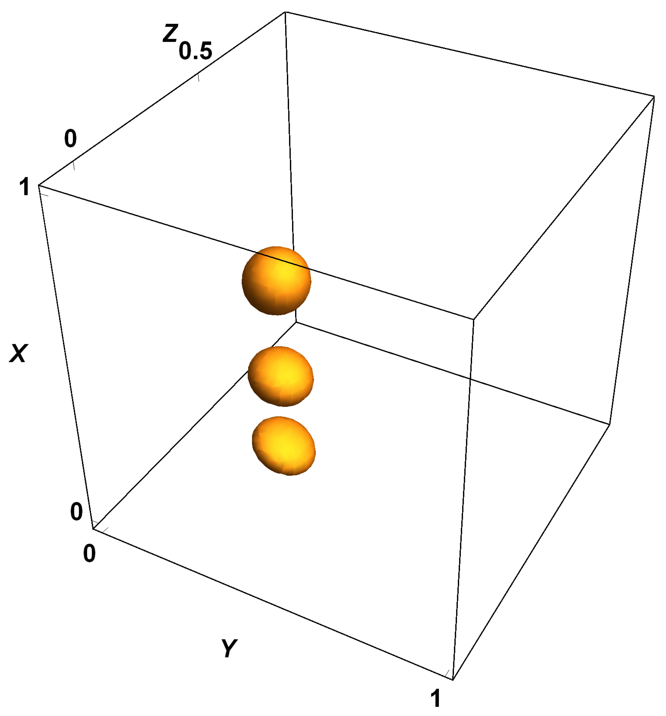
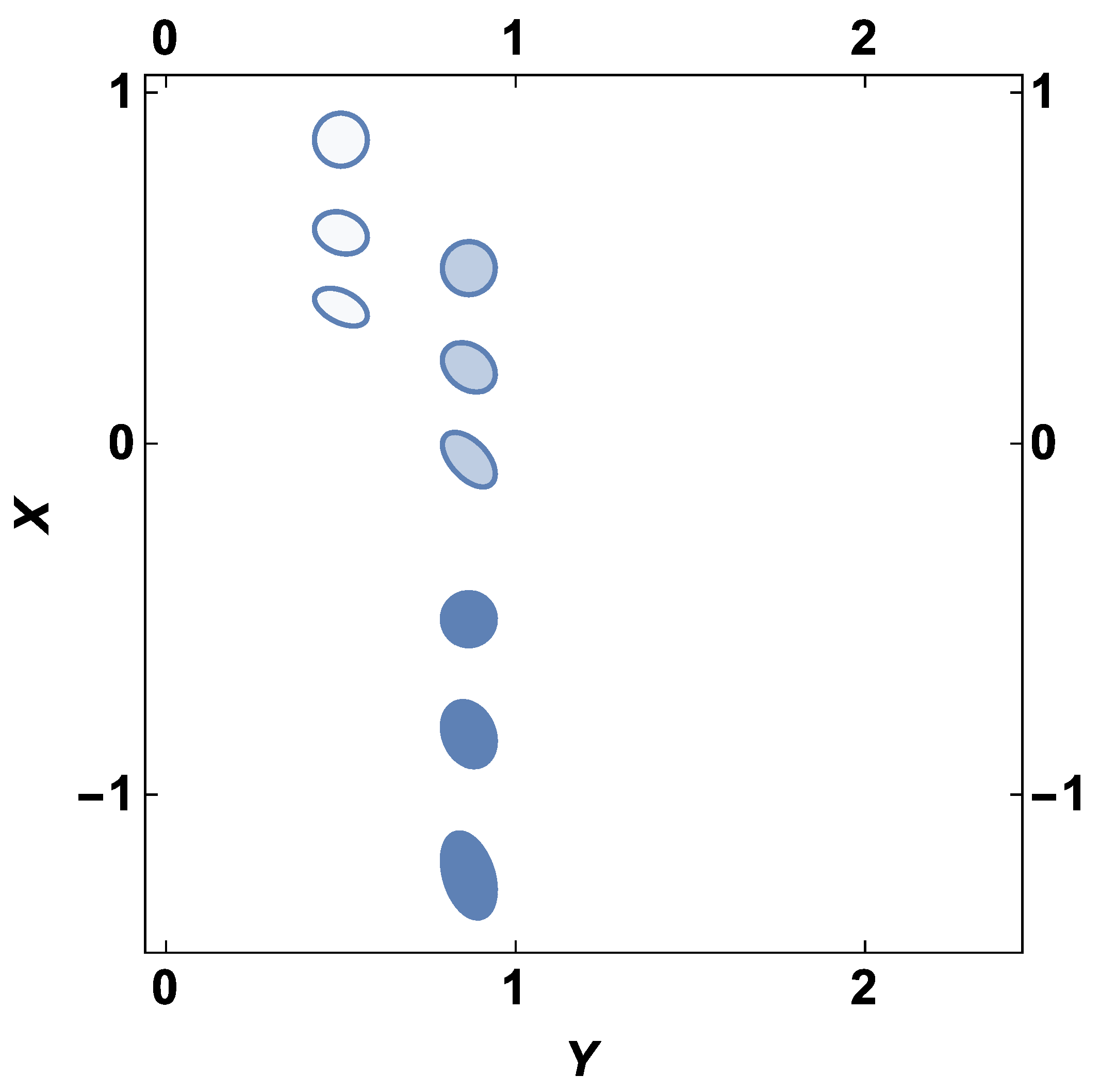
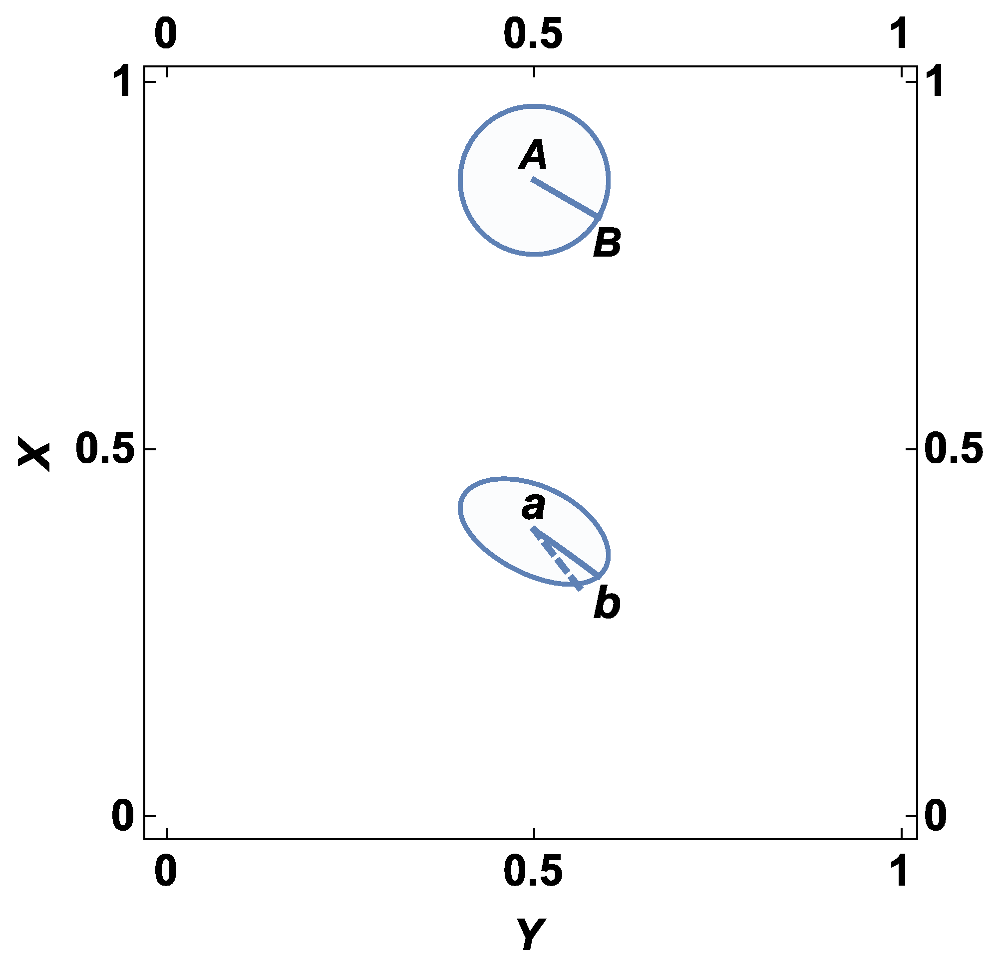
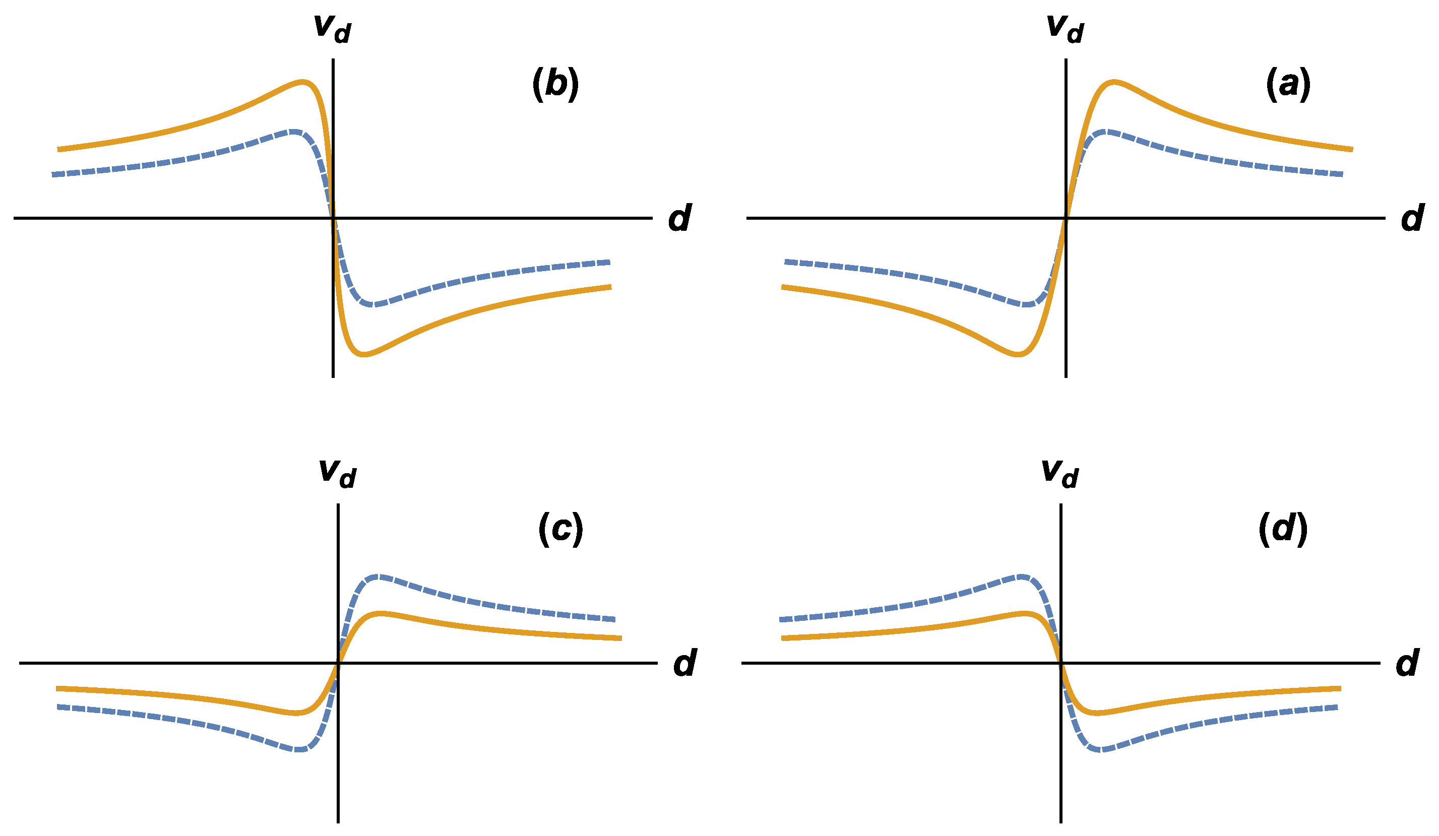
The theory, based on the concept in which the linear Hubble relation has the status of a fundamental law of small-scale cosmology, can be developed in different ways. In the present paper, the ‘small-scale cosmology’ is formulated as the theory operating in the $(z,\mathbf{r})$ (redshift–object coordinates) space. This allows developing a conceptual and computational basis of the theory along the lines of that of special relativity such that a complete one-to-one correspondence between the variables and relations of the two theories can be achieved. In pursuing the approach, the effectiveness of group theoretical methods is exploited. Applying the Lie group method yields transformations of the variables (the redshift and space coordinates of a cosmological object) between the reference frames of the accelerated observers. In this paper, the transformations are applied to studying the effects of the solar system observer acceleration on the observed shape, distribution and rotation curves of galaxy clusters.

This paper is organized as follows. In Section 2, following the introductory section, the framework of the small-scale cosmological model, patterned after special relativity, is developed, and the transformations relating the redshifts and space coordinates of an object measured by two accelerated observers are derived. (Some details of the derivation are placed in Appendix A). The particular case of the transformations, which relates the measurements made by inertial and accelerated observers, is specified. In Section 3, the transformations for that particular case are used to make conclusions about the influence of the observer acceleration on the observed shape, distribution and rotation curves of galaxy clusters. In Section 4, some comments on the conceptual framework of the theory and results are furnished.

2. Small-Scale Cosmology in the $(\mathit{z},\mathbf{r})$ Space

2.1. Framework

The underlying concept of the ‘small-scale cosmology’, as explained in the Introduction, is that the Hubble linear relation between the redshift of an extragalactic object and its distance is considered a universal law of nature which is used as the basis for the theory. For explaining the further development of the theory, let us make an excursus into the special relativity framework. The breakthrough in the development of special relativity was realizing that no absolute meaning, independent of the measurement procedure, can be assigned to such a quantity as the time of a remote event. In physics, before the relativity theory, different procedures were used to determine the time moment of a remote event, but it was considered a matter of course that all the procedures measure the same quantity which exists in itself. It was not realized that the assumptions related to different procedures correspond to different definitions of what the time of a remote event is. The relativity theory put forward the idea that the time moment of a remote event is what should be defined if one wishes to operate with that variable. This finding is of general value and, as a matter of fact, cannot be challenged. However, for developing a theory which could handle the experimental facts, the next step, choosing a specific definition for the time of a remote event, is needed, and in special relativity, the principle of universality of light propagation in inertial frames served as a basis for the definition. Combined with the relativity principle, it can be formulated as a statement that the times and coordinates of events vary from frame to frame in such a way that the light front, which is spherical in one inertial frame, remains spherical in any other inertial frame or, more generally, as the requirement of invariance of the equation of light propagation

$$c^{2}d{t}^2-d{r}^2=0$$

(8)

under the spacetime transformations between the frames of the inertial observers moving relative to each other.

Returning to cosmology, we find that the situation with the concept of the distance to a remote object is, in a sense, similar to that with the concept of time of a remote event in pre-relativistic physics; it is not completely realized that no pre-notion can be attributed to the distance to a remote object. Some clarifications regarding this statement are needed. It is usually admitted that it is impossible to give a natural notion of the distance in the universe on scales where space is curved. Different definitions of distance in a curved space, associated with the operational procedures used to measure the distance, lead to distances which are not equal to one another and are model-dependent. However, it is commonly stated that all of those definitions reduce to the usual notion of distance at low redshifts since the space becomes Euclidean. It is also taken for granted that at low redshifts, all internally self-consistent methods of measuring the distance must give the same result. The belief that on cosmologically small scales (low redshifts), a unique meaning can be assigned to the distance to a remote object, is what makes the situation similar to that with the notion of time of a remote event in physics before special relativity.

An unbiased analysis reveals that arguments supporting that belief are not valid. First, although it is usually not realized, the statement that the space at low redshifts is Euclidean is the model result. This result is obtained through an analytical continuation of the RWF cosmological model to small distances. In this respect, all of the above about the legitimacy of such a continuation in the context of validity of the Hubble law at small scales is relevant. The relations of the RWF cosmology rely on the assumptions of homogeneity and isotropy that evidently are not valid in the low-redshift universe.

Next, even in the Euclidean space, no absolute meaning, independent of the measurement procedure, can be assigned to the remote object distance. The ‘evidence’ that different methods of measuring the distance give the same result is an illusion. Each method involves some assumptions, particularly regarding the physical processes in the source and in the intergalactic matter. An agreement between the results, obtained by different methods, is achieved by introducing corrections into the assumptions, as is seen, for example, from the history of the SNe Ia calibration. In the process of adjusting the results, one method is taken as the basic one. In the calibration of the SNe Ia candles, it was the method based on the Hubble law.

Thus, one can conclude that even on cosmologically small scales, a definition of what the distance to a remote object is is needed. Each definition should be associated with an operational procedure, and thus for developing a consistent theory, one of the procedures should be chosen as a definition. The definition based on the Hubble law, adopted in the present theory, is a natural choice. With that definition, the ‘small-scale cosmology’, as the theory operating in the $(z,\mathbf{r})$ (redshift, object coordinates) space, can be developed along the lines of special relativity. The similarity of the theories begins at the level of concepts: a starting point of both theories is admiring the fact that one of the variables involved in the theory requires definition. What is more, there exists one-to-one correspondence between the variables taking part in the basic relations of the two theories. The Hubble law $z=Hr$ becomes identical to the equation of the light front $R=cT$ upon the replacement of the redshift z by the radial distance to the front R, the distance to the object r by the corresponding time moment T and the Hubble constant H by the speed of light c. The analogy is profound in that z and R are measurable quantities, while r and T are the variables that require definition. This correspondence may be considered a hint, suggesting that the framework of the present theory should be designed along the lines of special relativity.

The basic principle of special relativity is invariance of the equation of the light front, which can be written in a more general form (Equation (8)), covering the cases of the light waves propagating from and to the origin of the coordinates. The Hubble law, if not to make reservations regarding the sign of the wavelength shift, can be written in the form similar to Equation (8) as follows:

$$H^{2}d{\widehat{r}}^2-d{z}^2=0$$

(9)

where the coordinate $\widehat{r}$ (hats are used to mark dimensional variables) and the wavelength shift z play the same roles as t and r in Equation (8), respectively. This analogy serves as a guide for further development of the theory. The principle of invariance of the law of propagation of light (Equation (8)) with respect to the change in the state of motion of an observer suggests using a similar principle in the present theory, namely the invariance of the Hubble law (Equation (9)) with respect to the change in the observer’s state of motion. The kind of motions with which the theory should deal can also be defined using the analogy with special relativity. Special relativity deals with the inertial observers moving relative to each other with a constant velocity. If the frames of two inertial observers, say $S(X,Y,Z)$ and $S^{\prime }(x,y,z)$, in the standard configuration (with the y and z axes parallel to the Y and Z axes and the $S^{\prime }$ frame moving relative to S with a velocity v along the positive direction of the common x axis) are considered, then in the limit of small velocities $v\ll c$, the space and time variables of the observer frames are related to each other by the Galilean transformation

$$x-X=-vT$$

(10)

where T is an absolute time that is not transformed. Then, in light of the above stated correspondence between the variables in the two theories, in the ‘small-scale cosmology’, one has to consider a situation where a change of state of the motion of an observer results in a change in the redshift proportional to the distance to the source of radiation. As is shown below, based on the GR relations, this leads to the conclusion that accelerated observers should figure into the theory instead of uniformly moving observers of special relativity.

According to general relativity, the acceleration of an observer is equivalent to the appearance of the uniform gravitational field in the frame of the observer, and thus this results in a wavelength shift proportional to the distance to the source of the radiation. The frequency shift $\Delta \omega$ in the uniform gravitational field is given by [41]

$$\Delta \omega =\frac{{\varphi }_1-{\varphi }_2}{c^2}\omega$$

(11)

where $\omega$ is the frequency of light if it were emitted in an Earth laboratory and ${\varphi }_1$ and ${\varphi }_2$ are the potentials of the gravitational field at the points of emission and observation, respectively. With the x axis pointed in the direction of the observer acceleration, the gravitational field is pointed in the negative x direction, and thus, for the source with a coordinate $\widehat{x}$, (In order not to complicate matters, we, for a while, restrict ourselves to the sources on the x axis such that $\widehat{r}=\widehat{x}$) we have

$${\varphi }_1-{\varphi }_2=\left|g_{*}\right|\widehat{x}=\widehat{g}\widehat{x}$$

(12)

where $g_{*}$ is the strength of the gravitational field and $\widehat{g}$ is the observer acceleration. Then, for the wavelength shift, we obtain

$$z=\frac{\Delta \lambda }{\lambda }=-\frac{\Delta \omega }{\omega }=-\frac{\widehat{g}}{c^2}\widehat{x}$$

(13)

In this relation, $\widehat{g}$ is always positive, (The x axis is pointed in the direction of the acceleration), while $\widehat{x}$ may take on both positive and negative values, with the former corresponding to the objects seen by the observer in the direction of acceleration and the latter being for the objects seen in the opposite direction.

If there are two observers moving with accelerations $\widehat{G}$ and $\widehat{g}$ along a common $\widehat{x}$ axis, then the wavelength shifts in the observer frames are

$$Z=-\frac{\widehat{G}}{c^2}\widehat{X},z=-\frac{\widehat{g}}{c^2}\widehat{X}$$

(14)

Note that within the GR framework, the coordinate $\widehat{X}=\widehat{x}$ is not transformed. It follows from Equation (14) that

$$z-Z=-\frac{\widehat{g}-\widehat{G}}{c^2}\widehat{X}$$

(15)

Upon introducing nondimensional quantities defined by

$$r=\widehat{r}H,x=\widehat{x}H,X=\widehat{X}H,g=\frac{\widehat{g}}{c^{2}H},G=\frac{\widehat{G}}{c^{2}H}$$

(16)

Equation (15) takes the form

$$z-Z=-(g-G)X$$

(17)

It can immediately be seen that with the above noted correspondence of the variables figuring into the two theories, the relation in Equation (17) is similar to the relation in Equation (10) on special relativity, with the relative velocity v replaced by the relative acceleration $g-G$. Thus, as in special relativity, the relation in Equation (17) may be considered the small relative acceleration limit $|g-G|\ll 1$ of general transformations. It is important to note that there is a conceptual shift here like that in special relativity, where the absolute time is a notion having meaning only in the limiting case of the Galilean transformations (Equation (10)), while in the general transformations (Lorentz transformations), the time period elapsing in a remote event is different for the observers moving relative to each other. Similarly, in the ‘small-scale cosmology’, an ‘absolute’ distance is a notion applicable only to the limiting case in Equation (17), while in the general transformations, the distance to an object varies from observer to observer.

In the framework of special relativity, as was analyzed in [42], the relation in Equation (10) plays an important role. In the derivation of the transformations, which leave the equation of propagation of light (Equation (8)) invariant, a number of other physical requirements, such as associativity and reciprocity, should be satisfied by the transformations. All those requirements are covered by the condition that the spacetime transformations between inertial frames form a group. It was shown in [42] that invariance of the equation of light propagation and the group property of the transformations are not sufficient for obtaining the transformations in a complete form, and the most consistent way to complete the derivation is to complement the invariance of the light propagation and group property with the correspondence principle. In the context of special relativity, it is implied that in the limit of small velocities $v\ll c$, the formula for the coordinate transformation turns into that of the Galilean transformation (Equation (10)).

Note that commonly, in textbooks (see, for example, [43]), the condition of invariance of the interval between two events, complemented by the assumption of linearity of the transformations, is used. However, the invariance of the interval does not straightforwardly follow from the basic principles of the relativity theory. Therefore, using invariance of the interval is usually preceded by some arguments (see, for example, [41,43]) intended to justify the switch from invariance of the equation of light propagation to invariance of the interval. Nevertheless, those arguments cannot be considered a rigorous proof, and moreover, they are not always valid [42].

In the present analysis, the relation in Equation (17) plays the same role as Equation (10) in the special relativity analysis, with both of them defining the limiting cases according to the correspondence principle. Therefore, in the derivation of the transformations relating the redshifts and coordinates of an object, as measured by two accelerated observers, in addition to the requirements of invariance of Equation (9) and the group property, it is required that the transformation formula for z is turned into Equation (17) in the limit of small relative accelerations. (As a matter of fact, the limit of a small $g-G$ in Equation (17), like the limit of a small v in Equation (10), corresponds to small values of the group parameter).

2.2. Groups of Transformations

2.2.1. Line of Sight of an Object Is along the Acceleration Axis

We will start with the one-dimensional case where all the radiation sources are on the x axis. Then, the derivation of the transformations between the accelerated frames of two observers in the $(z,x)$ variables becomes completely similar to the derivation of the transformations (Lorentz transformations) between two inertial frames in special relativity in the $(x,t)$ variables. Let us consider two observers S and $S^{\prime }$ moving with accelerations G and g, respectively, with both directed along the x axis. The equations expressing the Hubble law in frames S and $S^{\prime }$ are

$$d{Z}^2-d{X}^2=0$$

(18)

$$d{z}^2-d{x}^2=0$$

(19)

A one-parameter (a) group of transformations converting Equation (18) into Equation (19) is sought in the form of

$$z=f(Z,X,G;a),x=q(Z,X,G;a);g=p(G;a)$$

(20)

It is important that in the subsequent analysis, the frame acceleration relative to an inertial frame is a variable that takes part in the group transformations. This in particular places the inertial frame with $G=0$ on equal footing with all accelerated frames, since the transformations to and from that frame become regular members of the group of transformations between accelerated frames. According to the infinitesimal Lie group method (see, for example, [44,45]), the infinitesimal transformations corresponding to Equation (20) are introduced as follows:

$$z\approx Z+\zeta (Z,X,G)a,x\approx X+\rho (Z,X,G)a,g\approx G+\gamma \left(G\right)a$$

(21)

Applying the correspondence principle, which requires that the transformation for the variable z turned into Equation (17) in the limit of small values of $(g-G)$ (a limit of a small a, as can be seen in the last relation of Equation (21)), allows one to define the form of the group generator $\zeta$ for the z variable. It is important that in the GR limit, the distance to a source and thus the coordinate x in the direction of acceleration are not transformed. (Like in special relativity, the variable T, a counterpart of R, is not transformed in the small a limit in Equation (10)) Then, the generator $\zeta$ is determined as follows:

$$z=Z+(G-g))X\Rightarrow Z+\zeta a=Z-\gamma (G)Xa\Rightarrow \zeta =-\gamma (G)X$$

(22)

Substituting the infinitesimal transformations defined by Equation (21), with $\zeta$ defined by Equation (22), into Equation (19) and linearizing the resulting relation with respect to a upon using Equation (18) to eliminate $d{Z}^2$ yields a polynomial in the differentials of the variables Z and X. Then, the requirement of vanishing coefficients of the monomials results in an overdetermined system of differential equations for the infinitesimals $\rho$ and $\gamma$, which is easily solved to give

$$\rho =-\gamma \left(G\right)Z$$

(23)

Finite transformations are determined by solving the Lie equations

$$\frac{dx\left(a\right)}{da}=-\gamma \left(g\left(a\right)\right)z\left(a\right),\frac{dz\left(a\right)}{da}=-\gamma \left(g\left(a\right)\right)x\left(a\right),\frac{dg\left(a\right)}{da}=\gamma \left(g\left(a\right)\right)$$

(24)

with the initial conditions

$$x\left(0\right)=X,z\left(0\right)=Z,g\left(0\right)=G$$

(25)

In light of the structure of the right-hand sides of the first two equations of Equation (24), it is convenient, using the last equation of Equation (24), to transform Equation (24) for the functions $x\left(a\right)$ and $z\left(a\right)$ to equations for the functions $x\left(g\right)$ and $z\left(g\right)$ of the variable $g\left(a\right)=g$ (the same notation for x and z is retained) as follows:

$$\frac{dx\left(g\right)}{dg}=-z\left(g\right),\frac{dz\left(g\right)}{dg}=-x\left(g\right),x\left(G\right)=X,z\left(G\right)=Z$$

(26)

The solution to the problem in Equation (26) is easily found in the form

$$\begin{array}{c}\hfill x=Xcosh(g-G)-Zsinh(g-G),\hfill \\ \hfill z=Zcosh(g-G)-Xsinh(g-G)\hfill \end{array}$$

(27)

It can be seen that the small $g-G$ limit of the second relation of Equation (27) is the first equation of Equation (22), which shows the consistency of the derivation.

Like in special relativity, where the interval is an invariant of the group of Lorentz transformations [42], in the present derivation, the combination $Inv=d{z}^2-d{r}^2$ is an invariant of the transformations in Equation (27) which may take any value. Therefore, the transformations are applicable not only to the objects with $z=r$, which corresponds to the zero value of $Inv$, but also to the objects with $z\ne r$ when redshifts due to peculiar velocities are imposed on the cosmological redshift $z=r$.

The transformations in Equation (27) include transformations from and to an inertial frame as regular members of the group of transformations between accelerated frames. In order to demonstrate this, let us obtain the transformation in Equation (27) by combining two transformations. Here, we should be accurate with the notation. The transformation from an inertial frame to an accelerated one is obtained by setting $G=0$ in Equation (27), but we have to replace g with $\tilde{g}$ and $(Z,X,z,x)$ with $(Z_i,X_i,z_r,x_r)$ as follows:

$$x_r=X_{i}cosh\tilde{g}-Z_{i}sinh\tilde{g},z_r=Z_{i}cosh\tilde{g}-X_{i}sinh\tilde{g}$$

(28)

where $Z_i$ and $X_i$ are the coordinates of the object in an inertial frame. Then, for the transformations from an inertial frame to two accelerated frames, with accelerations G and g, the parameter $\tilde{g}$ takes on the values G and g, while the coordinates $(z_r,x_r)$ take on the values $(Z,X)$ and $(z,x)$, respectively:

$$X=X_{i}coshG-Z_{i}sinhG,Z=Z_{i}coshG-X_{i}sinhG$$

(29)

$$x=X_{i}coshg-Z_{i}sinhg,z=Z_{i}coshg-X_{i}sinhg$$

(30)

It is readily verified that solving the two equations in Equation (29) for $X_i$ and $Z_i$ and substituting the solutions into Equation (30) yields the transformations in Equation (27). Thus, transformations from an inertial frame to an accelerated frame can be considered on equal footing with transformations between two accelerated frames.

2.2.2. Line of Sight of an Object Is Inclined to the Acceleration Axis

As in the previous section, two accelerated frames with accelerations G and g directed along the common x axis are considered, but the transformations are derived for a general case where the object is not on the line of accelerations. It is evident that there is an axial symmetry in such a configuration such that the position of the object is characterized by a radial distance r and a polar angle $\theta$, with $x=rcos\theta$ and $y=rsin\theta$ being the Cartesian coordinates in the $(r,\theta )$ plane. The transformed variables are $(z,r,\theta ,g)$, but in what follows, the variable $m=cos\theta$ is used instead of $\theta$. Thus, the transformations from $(Z,R,M,G)$ to $(z,r,m,g)$, with $M=cos\mathsf{\Theta }$ and $m=cos\theta$, which leave the Hubble law invariant, are considered. Derivation of the transformations proceeds along the lines of that in Section 2.2.1. In order not to overload the presentation, the details of the derivation have been placed into Appendix A below, and only the resulting transformations are given as follows:

$$r={\left({\left(MRcosh\left(g-G\right)-Zsinh\left(g-G\right)\right)}^2+\left(1-M^2\right)R^2\right)}^{1/2},$$

(31)

$$z=Zcosh(g-G)-MRsinh(g-G),$$

(32)

$$\begin{array}{c}m=\frac{MRcosh\left(g-G\right)-Zsinh\left(g-G\right)}{{\left({\left(MRcosh\left(g-G\right)-Zsinh\left(g-G\right)\right)}^2+\left(1-M^2\right)R^2\right)}^{1/2}}\end{array}$$

(33)

Note that the small $g-G$ limit of Equation (32) is in Equation (A6).

Also note that, similar to the one-dimansional case considered in the previous subsection, the combination $d{z}^2-d{r}^2$ is an invariant of the transformations in Equations (31)–(33), which may take any value and not only the zero value corresponding to the cosmological Hubble redshift. Therefore, the transformations are applicable not only to the objects with $z=r$ but also to the objects with $z\ne r$ when redshifts due to peculiar velocities are imposed on the Hubble redshift. The transformations in Equations (31)–(33) include transformations from or to an inertial frame as regular members of the group of transformations between accelerated frames. It can be shown in the same way as in the previous section that the transformations in Equations (31)–(33) can be derived by combining two transformations from an inertial frame to the accelerated G and g frames. Thus, we can use the particular case $G=0$ of the transformations in Equations (31)–(33) for defining transformations from an inertial frame to the frame moving with the acceleration g.

Finally, note that we do not consider the most general case where the accelerations of the two frames are not directed along the same line. The reason for not including derivation for this case is that in the applications considered in the next section, only the transformations from an inertial frame to an accelerated frame are used so that one acceleration direction figures into the analysis.

3. Applications

3.1. Relevant Accelerations

First, it is necessary to identify what could be accelerations, which are relevant to applications within the framework of the ‘small-scale cosmology’. Note again that the framework of cosmology in general implies averaging over a proper spacetime domain. In other terms, in cosmology, one is filtering the observed structure, retaining only the information on structures that are larger than that allowed by the filter. In cosmological models of the RW type, one smears over structures of the scale of galaxies and galaxy clusters such that the assumption that the distant universe is approximately uniform or homogeneous becomes supported by the observations. Similarly, the development of the universe over time is smoothed in those models such that the processes on the time scales of the processes occurring in galaxies and galaxy clusters are not addressed by the model equations. In the ‘small-scale cosmology’ developed in the present study, one smears over planets and stars such that the minimal-scale structures allowed by the filter are galaxies. This implies that the observed universe is smoothed over corresponding space and time scales. In particular, with such averaging, the accelerations on the small scales, such as the acceleration of the Earth observer due to the motion of the Earth around the Sun, cannot figure into the model. Thus, the relevant acceleration is the acceleration of the solar system’s barycenter with respect to the center of our galaxy.

The issue of measuring the solar system’S acceleration has obtained increased attention in recent years. It is closely related to one of the main endeavors of fundamental astrometry, namely establishing practical realization of an inertial reference frame anchored to celestial objects whose positions are defined by the barycentric coordinates of the solar system. The solar system’s acceleration can be determined through measuring the change in the aberration patterns of a light source (secular aberration), which is possible at the current level of astrometric observational accuracy. There are dozens of papers presenting estimates of the solar system’s acceleration using different methods (for recent results see, for example, [46,47,48,49]). According to the estimates, the solar system’s acceleration magnitude ($\widehat{g}$ in our notation) is within the interval $\widehat{g}=(2-3)\times {10}^{-10}$m/${\mathrm{s}}^2$, which gives for the nondimensional parameter g, defined in Equation (16) (with the Hubble constant value H = 75 km/s/Mpc), the interval g = 0.3–0.4. This indicates that the parameter g is of the order of one and, most likely, less than one.

3.2. Galaxy Clusters

Galaxy clusters are inherently multi-wavelength objects. Thanks to the simultaneous analysis of multi-wavelength data undertaken in the last 15 years or so, galaxy clusters have now become a widely used cosmological probe. Studies on galaxy clusters have proved crucial in helping to establish the standard model of cosmology, with a universe dominated by dark matter and dark energy. Also, they have been used to constrain various extensions of the minimal cosmological model, including the equation of state of dark energy, total mass of the neutrinos and modified gravity scenarios (e.g., [50,51,52,53,54,55]). Galaxy clusters have been used for cosmology in a variety of ways, such as by using information on their spatial distribution (e.g., [56]) or estimating their abundances as a function of the mass and redshift (e.g., [54]). These two methods have gained prominence in recent years. The results of the calculations presented below show that the parameters taking part in those methods should be influenced by the observer acceleration since the cluster’s position, mass concentration distribution and correspondingly three-dimensional shape change due to the acceleration. Thus, corrections for the effects of the observer acceleration should be introduced into calculations of the cosmological parameters determined using the galaxy cluster data.

3.3. Galaxy Cluster’s Shape and Position

Let us consider a galaxy cluster consisting of identical galaxies which do not have peculiar velocities (the cluster is not rotating) such that the redshifts in their spectra obey the Hubble law, which is $z=r$ in the present units. The following calculations are aimed at defining how a distribution of the cluster density (number of galaxies per unit volume) changes from an inertial to an accelerated frame. Then, the corresponding change of the cluster shape and position in space can be determined by defining the cluster boundary as a surface on which the density is smaller than some prescribed value. In this context, a particular case of the transformations in Equations (31)–(33), corresponding to the transformations from an inertial frame ($G=0$) to the accelerated frame, is to be applied, with the quantity g acquiring the meaning of the frame acceleration relative to an inertial frame. Setting $G=0$ in Equations (31)–(33) and specifying to the galaxies with $Z=R$ obeying the Hubble law yields

$$\begin{array}{c}r=R\left(coshg-Msinhg\right),m=\frac{Mcoshg-sinhg}{coshg-Msinhg},\hfill \\ m=cos\theta ,M=cos\mathsf{\Theta }\hfill \end{array}$$

(34)

where $(R,\mathsf{\Theta })$ are the coordinates of a galaxy in an inertial frame ($g=0$) and $(r,\theta )$ are the coordinates of the same galaxy in the accelerated frame ($g\ne 0$). (Note that for a galaxy obeying the Hubble law, Equations (31) and (32) become identical and reduce to the first equation of Equation (34).) For the calculations aimed at defining the three-dimensional cluster shape, the third spherical coordinate $\varphi$ is to be introduced. However, in light of the axial symmetry, that coordinate remains invariant under the transformations from an inertial to an accelerated frame:

$$\mathsf{\Phi }=\varphi$$

(35)

Equation (35) takes part in the calculations defining the density distribution in the accelerated frame, since the calculations involve converting the variables from Cartesian to spherical coordinates and vice versa.

Let $n(g,r_c,{\theta }_c,{\varphi }_c)$ be a distribution of the cluster density (a number of galaxies per unit volume) in the accelerated frame and $n_0(r_c,{\theta }_c,{\varphi }_c)=n(0,r_c,{\theta }_c,{\varphi }_c)$ be the density distribution in the inertial frame. Here and in what follows, $(r_c,{\theta }_c,{\varphi }_c)$ are the space spherical coordinates (defining the coordinate grid), while the notations $(R,\mathsf{\Theta },\mathsf{\Phi })$ and $(r,\theta ,\varphi )$ are reserved for the values of the coordinates of a specific galaxy in the inertial and accelerated frames. The cluster density distribution changes from $n_0(r_c,{\theta }_c,{\varphi }_c)$ in the inertial frame to $n(g,r_c,{\theta }_c,{\varphi }_c)$ in the accelerated frame due to a change in the galaxy coordinates, which results in the galaxy’s ‘movement’ through the coordinate grid $(r_c,{\theta }_c,{\varphi }_c)$. The ‘continuity equation’ for this ‘flow’ has the form

$$\begin{array}{c}\frac{\partial n}{\partial g}+\frac{\partial \left(n{V}_r\right)}{\partial r_c}+\frac{1}{r_c}\frac{\partial \left(n{V}_{\theta }\right)}{\partial {\theta }_c}=0\hfill \\ \to \frac{\partial n}{\partial g}+\frac{\partial \left(n{V}_r\right)}{\partial r_c}-\frac{1}{r_c}\sqrt{1-m_c^2}\frac{\partial \left(n{V}_{\theta }\right)}{\partial m_c}=0\hfill \end{array}$$

(36)

where $m_c=cos{\theta }_c$, and the ‘velocity’ vector is defined by

$$\left(V_r,V_{\theta }\right)={\left(\frac{\partial r}{\partial g},r\frac{\partial \theta }{\partial g}\right)}_{g=0}=\left(-m_c{r}_c,r_c\sqrt{1-m_c^2}\right)$$

(37)

Note that $V_{\varphi }=0$ since the coordinate $\varphi$ does not change in the transformation from an inertial to an accelerated frame.

The solution to the equation defined by Equations (36) and (37) satisfying the condition $n(0,r_c,m_c,{\varphi }_c)=n_0(r_c,m_c,{\varphi }_c)$ has the form

$$\begin{array}{c}n(g,r_c,m_c,{\varphi }_c)=n_0\left(I_1,I_2,{\varphi }_c\right);\hfill \\ I_1=\frac{1}{2}{e}^{-g}\left(1-m_c+e^{2g}\left(1+m_c\right)\right)r_c,\hfill \\ I_2=-1+\frac{2(1+m_c)}{1+m_c+e^{-2g}(1-m_c)}\hfill \end{array}$$

(38)

The shape of the galaxy cluster is defined by assigning the cluster boundary as a surface on which the density is smaller than some prescribed value. It is assumed that the cluster is of a spherical shape in an inertial frame, with the density distribution in Cartesian coordinates $(x,y,z_{car})$ having the form of King’s distribution [57]:

$$n_0^{\left(D\right)}(x,y,z_{car})=N_0{\left(1+\frac{{\left(x-x_0\right)}^2+{\left(y-y_0)\right)}^2+z_{car}^2}{R_c^2}\right)}^{-3/2}$$

(39)

where $(x_0,y_0,0)$ are the coordinates of the cluster center, $N_0$ is a constant and $R_c$ is a scale factor, which may be called the core radius. The distribution in Equation (39) fits the isothermal sphere and the data not too far from the central region quite well, and it adheres to the Newtonian behavior at larger distances. It is frequently used in theoretical modeling of galaxy cluster dynamics since this allows easy analytical computations (e.g., [58]). If the plane $\mathsf{\Phi }=0$ coincides with the plane $z_{car}=0$, and $R_0$ and ${\mathsf{\Theta }}_0$ are the coordinates of the cluster’s center in that plane, then the distribution in Equation (39) is written as follows:

$$n_0^{\left(D\right)}(x,y,z_{car})=N_0{\left(1+\frac{{\left(x-R_{0}cos{\mathsf{\Theta }}_0\right)}^2+{\left(y-R_{0}sin{\mathsf{\Theta }}_0\right)}^2+z_{car}^2}{R_c^2}\right)}^{-3/2}$$

(40)

The value of the constant $N_0$ is of no importance to the calculations intended for identifying changes related to the frame acceleration, and it is set to $N_0=1$ in what follows.

To determine the shape of the cluster in an accelerated frame, it is necessary to calculate the density distribution $n^{\left(D\right)}(g,x,y,z_{car})$ as transformed from the density distribution $n_0^{\left(D\right)}(x,y,z_{car})$ in an inertial frame. Since the transformation in Equation (38) is in spherical coordinates, the distribution $n_0^{\left(D\right)}(x,y,z_{car})$ should first be converted from Cartesian to spherical coordinates as follows:

$$n_0(r_c,m_c,{\varphi }_c)=n_0^{\left(D\right)}(r_c{m}_c,r_c\sqrt{1-m_c^2},r_c\sqrt{1-m_c^2}sin{\varphi }_c)$$

(41)

Next, the transformation in Equation (38) is applied, which yields

$$\begin{array}{c}n\left(g,r_c,m_c,{\varphi }_c\right)=n_0(\frac{1}{2}{e}^{-g}\left(1-m_c+e^{2g}\left(1+m_c\right)\right)r_c\hfill \\ -1+\frac{2(1+m_c)}{1+m_c+e^{-2g}(1-m_c)},{\varphi }_c)\hfill \end{array}$$

(42)

Finally, the distribution $n\left(g,r_c,m_c,{\varphi }_c\right)$ is transformed from spherical coordinates to Cartesian coordinates as follows:

$$n^{\left(D\right)}(g,x,y,z_{car})=n\left(g,\sqrt{x^2+y^2},\frac{x}{\sqrt{x^2+y^2}},arctan\left(\frac{z_{car}}{y}\right)\right)$$

(43)

The results are presented in Figure 1 and Figure 2, which show how the cluster’s shape and position change when the acceleration parameter g increases. In Figure 1, this is shown in three dimensions for one particular case (see the caption), and in Figure 2, this is shown in the cross-section $z_{car}=0$ for three different positions of the cluster in an inertial frame. It is seen, first of all, that a cluster having a spherically symmetric shape in an inertial frame looks prolate to an observer in the accelerated frame. The exact form of galaxy clusters is still debated in the literature. However, it is generally accepted, based on X-ray and gravitational lensing studies, that they are triaxial in their shape [59,60,61,62]. The results of the present study show that any model designed for explaining the cluster ellipticity should take into account that the clusters already look prolate because of the observer acceleration.

Next, it can be seen in Figure 1 and Figure 2 that the change in the cluster shape from spherical to elliptical is accompanied by a change in the cluster size. If defining the ‘Northern Pole’ as the point to which the acceleration vector is directed, then one can say that for the clusters lying in an inertial frame in the ‘Northern’ hemisphere, the cluster size decreases when g increases, and the cluster size increases with g for clusters lying in the ‘Southern’ hemisphere. Thus, under the assumption that all the clusters have the same size in an inertial frame, one should expect that the clusters in the ‘Northern’ hemisphere, observed by an accelerated observer, should, in general, be smaller than those in the ‘Southern’ hemisphere. It can also be seen in Figure 1 and Figure 2 that, with g increasing, the position of the cluster in space changes such that the coordinate x decreases while the coordinate y remains constant, according to the relation in Equation (A4). Therefore, the polar angle $\theta$, under which a cluster can be seen for an observer in the accelerated frame, is larger than that in an inertial frame, while the distance to a cluster decreases with the acceleration for clusters in the ‘Northern’ hemisphere and increases for clusters in the ’Southern’ hemisphere. In general, it is expected that, with the uniform distribution of clusters in an inertial frame, the ‘Southern’ hemisphere should be more populated than the ‘Northern’ one for an observer in the accelerated frame.

3.4. Cluster Rotation Curves

As an application of the transformations in Equations (31)–(33) to the objects with $Z\ne R$, let us consider the rotating galaxy clusters. The cluster rotation should be taken into account in the calculation of the cluster masses, which is of the utmost importance for cosmological studies. The mass function and its evolution have been recognized as a rather important cosmological probe that can constrain the current cosmological model (e.g., [63,64,65]).

For a rotating galaxy cluster, a redshift of a particular galaxy at the distance R is a sum of the cosmological redshift $Z=R$ and the redshift, related to the peculiar galaxy velocity due to rotation of the cluster. It is assumed that the cluster has a spherical shape in an inertial frame. In what follows, a particular case where the rotation axis is normal to the plane defined by the line of acceleration (the x axis) and the line of sight of the cluster center is considered, while the transformations are applied to the galaxies lying in that plane on the diameter normal to the line of sight in an inertial frame. The rotation velocity vector of a galaxy is directed normal to that diameter, but the corresponding redshift is determined by its line of sight component $v_s$. The whole redshift is the sum of the cosmological redshift R and $v_s$ (which can be both positive and negative). In the following calculations, the law defining the dependence of the rotation velocity magnitude on the distance from the center in an inertial frame is taken in the form

$$v_d=S\frac{d}{{\left(1+{\left(d/R_c\right)}^2\right)}^{3/4}}$$

(44)

where d can be both positive and negative. The law in Equation (44) can be obtained (see, for example, [58]) by applying the virial theorem to the dynamically relaxed (virialized) cluster while calculating the mass of the cluster using the King’s profile density distribution (Equation (40)). A value of the constant S is of no importance in our calculations aimed at determining how the rotation velocity distribution (Equation (44)) changes due to the observer acceleration, which is set to $S=1$ in what follows. If the coordinates of the cluster center in an inertial frame are $(R_0,{\mathsf{\Theta }}_0)$, then the coordinates $(R,\mathsf{\Theta })$ of a galaxy lying on the diameter normal to the line of sight of the cluster center at the distance d from the center are related to $R_0$, ${\mathsf{\Theta }}_0$ and d by

$$R=\frac{R_0}{cos(\mathsf{\Theta }-{\mathsf{\Theta }}_0)},d=R_{0}tan(\mathsf{\Theta }-{\mathsf{\Theta }}_0)$$

(45)

and the redshift Z is calculated as follows:

$$Z=R+v_{d}cos(\mathsf{\Theta }-{\mathsf{\Theta }}_0)$$

(46)

where $v_d$ is defined by Equation (44).

To determine the rotation velocity distribution in the frame moving with the acceleration g, we will use the transformations of the galaxy coordinates and the corresponding redshifts from their values $(R,\mathsf{\Theta },Z)$ in an inertial frame to the values $(r,\theta ,z)$ in the g frame (the coordinate $\varphi$ is not transformed). The transformations from an inertial frame to the accelerated one are obtained by setting $G=0$ in the general transformations in Equations (31)–(33), which yields

$$r={\left({\left(MRcoshg-Zsinhg\right)}^2+\left(1-M^2\right)R^2\right)}^{1/2},$$

(47)

$$z=Zcoshg-MRsinhg,$$

(48)

$$m=\frac{MRcoshg-Zsinhg}{{\left({\left(MRcoshg-Zsinhg\right)}^2+\left(1-M^2\right)R^2\right)}^{1/2}}$$

(49)

where $M=cos\mathsf{\Theta }$ and $m=cos\theta$. The coordinates of the central point $(r_0,{\theta }_0)$, at which $z=r$, are calculated using the simplified relations in Equations (47) and (49) as follows:

$$r_0=R_0\left(coshg-M_{0}sinhg\right),$$

$$\begin{array}{c}\hfill m_0=\frac{M_{0}coshg-sinhg}{coshg-M_{0}sinhg},\hfill \end{array}$$

(50)

$$\begin{array}{c}\hfill m_0=cos{\theta }_0,M_0=cos{\mathsf{\Theta }}_0\hfill \end{array}$$

(51)

Calculating the coordinates $(r,\theta )$ and redshift z for the galaxies, which lie on the diameter normal to the line of sight of the cluster center in an inertial frame, shows that despite the substantial change in the coordinates of the central point from the inertial to the accelerated frame, in the accelerated frame, the galaxies lie on the (approximately) straight line inclined at a small angle to the line normal to the line of sight of the central point of the cluster (see Figure 3 and Figure 4). The distances from the central point to the galaxies along that line are calculated as follows:

$$d={\left(r^2+r_0^2-2r{r}_{0}cos\left(\theta -{\theta }_0\right)\right)}^{1/2}$$

(52)

The rotation velocity of a galaxy is determined from its line of sight component, calculated by subtracting the cosmological redshift r from the whole redshift value z, which yields

$$v_d=\frac{\left(z-r\right)d}{r_{0}sin\left(\theta -{\theta }_0\right)}$$

(53)

For given g, $R_0$, ${\mathsf{\Theta }}_0$ and $d_c$ values, the quantities r, $\theta$, $r_0$, ${\theta }_0$ and z, which take part in Equations (52) and (53), are determined by the relations in Equations (44)–(51), with $\mathsf{\Theta }$ being the running parameter for the parametric curve $v_d\left(d\right)$.

The results are presented in Figure 5. It can be seen that the influence of the observer acceleration on the shape of the rotation curves is different for clusters lying in the ‘Northern’ and ‘Southern’ hemispheres in an inertial frame. The rotation velocities of the clusters in the ‘Northern’ hemisphere increase because of the observer acceleration, which may have correlation with the issue of higher-than-expected velocities observed in clusters of galaxies. At the same time, for the clusters lying in the ‘Southern’ hemisphere in the inertial frame, the observer acceleration should result in lower velocities than those observed in the inertial frame.

4. Discussion

In the present paper, the ‘small-scale cosmology’ was developed as an independent theory, having no relation to the standard cosmology based on the RWF-type models. In the theory, the linear Hubble law status changes from the common interpretation of a small z limit of the RWF model or an effect of expanding space to the basis of the theory. The reasoning behind this is that, contrary to what is commonly accepted, validity of the linear Hubble law at cosmologically small scales cannot be proven using the global RWF cosmological models that are based on the assumptions of homogeneity and isotropy. Those assumptions are supported by observations only upon averaging the observational data over the scales, which are much larger than those with which the ‘small-scale cosmology’ deals such that small-scale structures like galaxies and clusters of galaxies are filtered out. For the same reason, extending the notions of dark matter and dark energy, which are introduced as the cosmic fluid density components in global large-scale dynamics of the universe, to small scales is conceptually inconsistent.

Development of the theory is based on the requirement that the Hubble law should be invariant with respect to a change in the observer acceleration. In pursuing this approach, the effectiveness of group theoretical methods, particularly the Lie group method, is exploited. The variables taking part in the transformations are the redshift and the distance (more precisely, the space coordinates) characterizing a cosmological object. This implies that the distance to the cosmological object is not something ‘absolute’ but relative and depending on the observer reference system. This leads to a profound change in the way we perceive space, similar to the conceptual change introduced by the theory of relativity. In both cases, it is in disagreement with the ‘common sense’ that we use regarding space and time measurements. In particular, regarding the distance to an object as something self-evident is apparently a result of transferring the picture of the physical space, obtained from experiments in our closed surroundings, to cosmological scales. Thinking about the distance to an object, we (unconsciously) represent to ourselves either repeated application of the measuring rod along the line of sight or the movements that must take place to reach the object (see the discussion in [66]). However, when comparing the scales of our even cosmic experience (e.g., distances to the closest planets) with those for cosmologically nearby objects, one can see by how many orders of magnitude the quantities differ. It is possible that applying the notions deduced from the accessible physical space experience to cosmology is similar to applying the concepts of the macroworld to the microworld of quantum theory and vice versa, and thus it could be expected that, like in the latter case, quantitative differences may result in qualitative changes.

Claiming the Hubble law to be the basic equation of the theory, which is formulated in the $(z,\mathbf{r})$ space, allows developing the theory along the lines of special relativity, where universality of the law of propagation of light is one of basic principles. The similarity reveals itself first in the possibility to establish the one-to-one correspondence between the variables taking part in the Hubble law and in the law of propagation of light, as well as how in both laws, one of the variables requires definition, and those variables in the two laws are in correspondence with each other. Therefore, there are grounds to develop the ‘small-scale cosmology’ maintaining that analogy. Of course, using the similarity of the basic law of the present theory with that of special relativity for development of the theory is a heuristic argument. Note, however, that it is not a rare situation in science where the approach and methods of one theory appear to be fruitful in another one. Thus, it is natural to expect that applying the concepts and methods which led to the well-established results in special relativity should result in meaningful consequences in its counterpart.

It is worth clarifying that the change in the redshifts in the spectra of galaxies due to the observer acceleration is not an effect similar to the Doppler redshift. The redshift in the spectra of galaxies, both before the observer acceleration and after it, is not attributed to the galaxies’ motion with respect to the observer frame; it is the cosmological redshift. Commonly, the cosmological redshift is attributed to space dilatation, but as discussed in the Introduction, applying the concept of space expansion on small scales is inconsistent and physically meaningful. In the ‘small-scale cosmology’, the change in the redshift induced by a change in the observer acceleration is a consequence of the invariance of the universal Hubble law, like how the dependence of the distances on the relative speed of the observers in special relativity is a consequence of the universality and invariance of the law of propagation of light.

In the present paper, the ‘small-scale cosmology’ was designed as a theory operating in the $(z,\mathbf{r})$ space. It would also be of interest to develop the theory, based on the concept of universality of the Hubble law, in the $(t,\mathbf{r})$ space, which should allow one to define the spacetime metric of the ‘small-scale cosmology’. The requirement of linearity of the relation between the redshift and a distance could be used to (partially) specify the components of the spacetime metric tensor. To further specify the metric, the ‘cosmological principle’ can be applied. The cosmological principle, in its general formulation, states that for any observer in the universe, the observations should yield the same results. In the context of large-scale cosmological models, the cosmological principle evolves to the statement that the universe, on average, should look isotropic and homogeneous for sets of ‘privileged’ observers, but it is irrelevant to the small scales. On the small scales, the cosmological principle implies that observations made by an observer in any galaxy should yield the same Hubble law, with the same Hubble constant as that determined by the observations made from our vantage point. (In some textbooks (e.g., [67]), one can find a ‘proof’ of this assertion, but the proof is invalid in the present context since it relies on the interpretation of the redshift as a recession velocity.) To apply the cosmological principle to development of the theory, the principle should be formulated as the condition of invariance of the spacetime metric with respect to a change in the observer’s location. This condition should impose restrictions on the components of the spacetime metric tensor, in addition to those imposed by the requirement of validity of the linear Hubble law. As a result, the spacetime (and space) metric would be (at least partially) defined, which in particular would allow revealing whether the statement that the space is Euclidean at small scales is compatible with the linearity of the redshift–distance relation.

To conclude, in this paper, the new conceptual view of cosmology at small scales, as a theory independent of the standard model of cosmology, is presented. The ‘small-scale cosmology’, based on that view, does not suggest any kinematical or dynamical interpretation neither for the redshift, considered a characteristic of an object, nor for the Hubble law, considered a physical reality. Nevertheless, it (like the large-scale cosmography) provides a theoretical framework for interpreting the observations and allows making some predictions, particularly regarding the influence of the observer acceleration on the observed shapes, distributions and rotation curves of the galaxy clusters.

References

1. Weinberg, S. Gravitation and Cosmology: Principles and Applications of the General Theory of Relativity; John Wiley & Sons, Inc.: New York, NY, USA, 1972. [Google Scholar]
2. Weinberg, S. Cosmology; Oxford University Press: Oxford, MA, USA, 2008. [Google Scholar]
3. Perlmutter, S.; Aldering, G.; Goldhaber, G.; Knop, R.A.; Nugent, P.; Castro, P.G.; Deustua, S.; Fabbro, S.; Goobar, A.; Groom, D.E.; et al. Measurements of Ω AND Λ from 42 high-redshift supernovae. Astrophys. J. 1999, 517, 565. [Google Scholar] [CrossRef]
4. Riess, A.G.; Filippenko, A.V.; Challis, P.; Clocchiattia, A.; Diercks, A.; Garnavich, P.M.; Gilliland, R.L.; Hogan, C.J.; Jha, S.; Kirshner, R.P.; et al. Observational evidence from supernovae for an accelerating universe and a cosmological constant. Astron. J. 1998, 116, 1009. [Google Scholar] [CrossRef]
5. Phillips, M.M. The Absolute Magnitudes of Type IA Supernovae. Astrophys. J. 1993, 413, L105. [Google Scholar] [CrossRef]
6. Riess, A.G.; Press, W.H.; Kirshner, R.P. Using Type IA Supernova Light Curve Shapes to Measure the Hubble Constant. Astrophys. J. 1995, 438, L17. [Google Scholar] [CrossRef]
7. Riess, A.G.; Press, W.H.; Kirshner, R.P. A Precise Distance Indicator: Type Ia Supernova Multicolor Light Curve Shapes. Astrophys. J. 1996, 473, 88. [Google Scholar] [CrossRef]
8. Riess, A.G.; Filippenko, A.V.; Leonard, D.C.; Schmidt, B.P.; Suntzeff, N.; Phillips, M.M.; Schommer, R.; Clocchiatti, A.; Kirshner, R.P.; Garnavich, P.; et al. Time Dilation from Spectral Feature Age Measurements of Type Ia Supernovae. Astron. J. 1997, 114, 722. [Google Scholar] [CrossRef]
9. Phillips, M.M.; Lira, P.; Suntzeff, N.B.; Schommer, R.A.; Hamuy, M.; Maza, J. The reddening-free decline rate versus luminosity relationship for type Ia supernovae. Astron. J. 1999, 118, 1766. [Google Scholar] [CrossRef]
10. Filippenko, A.V. Type Ia supernovae and cosmology. In White Dwarfs: Cosmological and Galactic Probes; Sion, E.M., Vennes, S., Shipman, H.L., Eds.; Springer: Heidelberg, The Netherlands, 2005; p. 97. [Google Scholar]
11. Harrison, E. Cosmology: The Science of the Universe; Cambridge University Press: Cambridge, UK, 2000. [Google Scholar]
12. Whiting, A.B. The Expansion of Space: Free Particle Motion and the Cosmological Redshift. Observatory 2004, 124, 174. [Google Scholar]
13. Peacock, J.A. A diatribe on expanding space. arXiv 2008, arXiv:0809.4573v1. [Google Scholar] [CrossRef]
14. Barnes, L.A.; Francis, M.J.; James, J.B.; Lewis, G.F. Joining the Hubble flow: Implications for expanding space. Mon. Not. R. Astron. Soc. 2006, 373, 382. [Google Scholar] [CrossRef]
15. Chodorowski, M.J. A direct consequence of the Expansion of Space? Mon. Not. R. Astron. Soc. 2007, 378, 239. [Google Scholar] [CrossRef]
16. Kaiser, N. Astronomical redshifts and the expansion of space. Mon. Not. R. Astron. Soc. 2014, 438, 2456. [Google Scholar] [CrossRef]
17. Rees, M.J.; Weinberg, S. All you ever wanted to know about the big bang. New Sci. 1993, 1869, 32. [Google Scholar]
18. Francis, M.J.; Barnes, L.A.; James, J.B.; Lewis, G.F. Expanding Space: The Root of all Evil? Publ. Astron. Soc. Aust. 2007, 24, 95. [Google Scholar] [CrossRef]
19. Andersson, L.; Coley, A. Inhomogeneous cosmological models and averaging in cosmology: Overview. Class. Quantum Grav. 2011, 28, 160301. [Google Scholar] [CrossRef]
20. Wiltshire, D.L. What is dust?—Physical foundations of the averaging problem in cosmology. Class. Quantum Grav. 2011, 28, 164006. [Google Scholar] [CrossRef]
21. Maartens, R. Is the Universe homogeneous? Phil. Trans. Roy. Soc. Lond. A 2011, 369, 5115. [Google Scholar] [CrossRef]
22. Umeh, O. Consequences of using a smooth cosmic distance in a lumpy universe. I. Phys. Rev. D 2022, 106, 023514. [Google Scholar] [CrossRef]
23. Coley, A.A.; Ellis, G.F.R. Theoretical cosmology. Class. Quantum Grav. 2020, 37, 013001. [Google Scholar] [CrossRef]
24. Trimble, V. Existence and nature of dark matter in the universe. Annu. Rev. Astron. Astrophys. 1987, 25, 425. [Google Scholar] [CrossRef]
25. Corbelli, E.; Salucci, P. The extended rotation curve and the dark matter halo of M33. Mon. Not. R. Astron. Soc. 2000, 311, 441. [Google Scholar] [CrossRef]
26. Faber, S.M.; Jackson, R.E. Velocity dispersions and mass-to-light ratios for elliptical galaxies. Astrophys. J. 1976, 204, 668. [Google Scholar] [CrossRef]
27. Carr, B.J.; Clesse, S.; García-Bellido, J.; Hawkins, M.R.S.; Kühnel, F. Observational evidence for primordial black holes: A positivist perspective. Phys. Rep. 2024, 1054, 1. [Google Scholar] [CrossRef]
28. Bird, S.; Albert, A.; Dawson, W.; Ali-Haïmoud, Y.; Coogan, A.; Drlica-Wagner, A.; Feng, Q.; Inman, D.; Inomata, K.; Kovetz, E.; et al. Primordial black hole dark matter. Phys. Dark Univ. 2023, 41, 101231. [Google Scholar] [CrossRef]
29. Hütsi, G.; Raidal, M.; Urrutia, J.; Vaskonen, V.; Veermäe, H. Did JWST observe imprints of axion miniclusters or primordial black holes? Phys. Rev. D. 2023, 107, 043502. [Google Scholar] [CrossRef]
30. Boylan-Kolchin, M.; James, S.; Bullock, J.S.; Kaplinghat, M. The Milky Way’s bright satellites as an apparent failure of ΛCDM. Mon. Not. R. Astron. Soc. 2012, 422, 1203. [Google Scholar] [CrossRef]
31. Kroupa, P. Galaxies as simple dynamical systems: Observational data disfavor dark matter and stochastic star formation. Can. J. Phys. 2015, 93, 169. [Google Scholar] [CrossRef]
32. Pawlowski, M.S.; Famaey, B.; Jerjen, H.; Merritt, D.; Kroupa, P.; Dabringhausen, J.; Lüghausen, F.; Forbes, D.A.; Hensler, G.; Hammer, F.; et al. Co-orbiting satellite galaxy structures are still in conflict with the distribution of primordial dwarf galaxies. MNRAS 2014, 442, 2362. [Google Scholar] [CrossRef]
33. Zavala, J.; Jing, Y.P.; Faltenbacher, A.; Yepes, G.; Hoffman, Y.; Gottlober, S.; Catinella, B. The velocity function in the local evironment from ΛCDM and ΛWDM constrained simulations. Astrophys. J. 2009, 700, 1779. [Google Scholar] [CrossRef]
34. Bull, P.; Akrami, Y.; Adamek, J.; Baker, T.; Bellini, E.; Jiménez, J.B.; Bentivegna, E.; Camera, S.; Clesse, S.; Davis, J.H.; et al. Beyond ΛCDM: Problems, solutions, and the road ahead. Phys. Dark Univ. 2016, 12, 56. [Google Scholar] [CrossRef]
35. Burde, G.I. Cosmological models based on relativity with a privileged frame. Int. J. Mod. Phys. D 2020, 29, 2050038. [Google Scholar] [CrossRef]
36. Burde, G.I. Particle dynamics and GZK limit in relativity with a preferred frame. Astropart. Phys. 2021, 126, 102526. [Google Scholar] [CrossRef]
37. Burde, G.I. Lorentz Violation by the Preferred Frame Effects and Cosmic and Gamma Ray Propagation. Galaxies 2021, 9, 119. [Google Scholar] [CrossRef]
38. Aghanim, N.; Akrami, Y.; Ashdown, M.; Aumont, J.; Baccigalupi, C.; Ballardini, M.; Banday, A.J.; Barreiro, R.B.; Bartolo, N.; Basak, S.; et al. Planck 2018 results. VI. Cosmological parameters. Astron. Astrophys. 2020, 641, A6. [Google Scholar]
39. Riess, A.G.; Macri, L.M.; Hoffmann, S.L.; Scolnic, D.; Casertano, S.; Filippenko, A.V.; Tucker, B.E.; Reid, M.J.; Jones, D.O.; Silverman, J.M.; et al. A 2.4% determination of the local value of the Hubble constant. Astrophys. J. 2016, 826, 56. [Google Scholar] [CrossRef]
40. Riess, A.G.; Casertano, S.; Yuan, W.; Macri, L.M.; Scolnic, D. Large magellanic cloud Cepheid standards provide a 1% foundation for the determination of the Hubble constant and stronger evidence for physics beyond ΛCDM. Astrophys. J. 2019, 876, 85. [Google Scholar] [CrossRef]
41. Landau, L.D.; Lifshitz, E.M. The Classical Theory of Fields; Pergamon Press: Oxford, UK, 1971. [Google Scholar]
42. Burde, G.I. Special relativity kinematics with anisotropic propagation of light and correspondence principle. Found. Phys. 2016, 46, 1573. [Google Scholar] [CrossRef]
43. Pauli, W. Theory of Relativity, 1958th ed.; Pergamon Press Ltd.: Oxford, UK, 1921. [Google Scholar]
44. Bluman, G.W.; Kumei, S. Symmetries and Differential Equations, Applied Mathematical Sciences; Springer: New York, NY, USA, 1989; Volume 81. [Google Scholar]
45. Olver, P.J. Applications of Lie Groups to Differential Equations (Graduate Texts in Mathematics); Springer: New York, NY, USA, 1993; Volume 107. [Google Scholar]
46. Titov, O.; Krasna, H. Measurement of the solar system acceleration using the Earth scale factor. Astron. Astrophys. 2018, 610, A36. [Google Scholar] [CrossRef]
47. MacMillan, D.S.; Fey, A.; Gipson, J.M.; Gordon, D.; Jacobs, C.S.; Krásná, H.; Lambert, S.B.; Malkin, Z.; Titov, O.; Wang, G.; et al. Galactocentric acceleration in VLBI analysis Findings of IVS WG8. Astron. Astrophys. 2019, 630, A93. [Google Scholar] [CrossRef]
48. Charlot, P.; Jacobs, C.S.; Gordon, D.; Lambert, S.; de Witt, A.; Böhm, J.; Fey, A.L.; Heinkelmann, R.; Skurikhina, E.; Titov, O.; et al. The third realization of the International Celestial Reference Frame by very long baseline interferometry. Astron. Astrophys. 2020, 644, A159. [Google Scholar] [CrossRef]
49. Klioner, S.A.; Mignard, F.; Lindegren, L.; Bastian, U.; McMillan, P.J.; Hernández, J.; Hobbs, D.; Ramos-Lerate, M.; Biermann, M.; Bombrun, A.; et al. Acceleration of the Solar System from Gaia astrometry. Astron. Astrophys. 2021, 649, A9. [Google Scholar]
50. Allen, W.; August, E.E.; Mantz, A.B. Cosmological parameters from observations of galaxy clusters. Annu. Rev. Astron. Astrophys. 2011, 49, 409. [Google Scholar] [CrossRef]
51. Cataneo, M.; Rapetti, D.; Schmidt, F.; Mantz, A.B.; Allen, S.W.; Applegate, D.E.; Kelly, P.L.; von der Linden, A.; Morris, R.G. New constraints on f(R) gravity from clusters of galaxies. Phys. Rev. D 2015, 92, 044009. [Google Scholar] [CrossRef]
52. Mantz, A.B.; von der Linden, A.; Allen, S.W.; Applegate, D.E.; Kelly, P.L.; Morris, R.G.; Rapetti, D.A.; Schmidt, R.W.; Adhikari, S.; Allen, M.T.; et al. Weighing the giants-IV. Cosmology and neutrino mass. Mon. Not. Roy. Astron. Soc. 2015, 446, 2205. [Google Scholar] [CrossRef]
53. Bohringer, H.; Chon, G. Constraints on neutrino masses from the study of the nearby large-scale structure and galaxy cluster counts. Mod. Phys. Lett. 2016, 31, 1640008. [Google Scholar] [CrossRef]
54. Bocquet, S.; Dietrich, J.P.; Schrabback, T.; Bleem, L.E.; Klein, M.; Allen, S.W.; Applegate, D.E.; Ashby, M.L.N.; Bautz, M.; Bayliss, M.; et al. Cluster Cosmology Constraints from the 2500 deg2 SPT-SZ Survey: Inclusion of Weak Gravitational Lensing Data from Magellan and the Hubble Space Telescope. Astrophys. J. 2019, 878, 55. [Google Scholar] [CrossRef]
55. Tanseri, I.; Hagstotz, S.; Vagnozzi, S.; Giusarma, E.; Freese, K. Updated neutrino mass constraints from galaxy clustering and CMB lensing-galaxy cross-correlation measurements. J. High Energy Astrophys. 2022, 36, 1–26. [Google Scholar] [CrossRef]
56. Marulli, F.; Veropalumbo, A.; Sereno, M.; Moscardini, L.; Pacaud, F.; Pierre, M.; Plionis, M.; Cappi, A.; Adami, C.; Alis, S.; et al. The XXL Survey. XVI. The clustering of X-ray selected galaxy clusters at z∼0.3. Astron. Astrophys. 2018, 620, A1. [Google Scholar] [CrossRef]
57. King, I.R. Density data and emission measure for a model of the Coma cluster. Astron. J. 1972, 174, L123. [Google Scholar] [CrossRef]
58. Manolopoulou, M.; Plionis, M. Galaxy cluster’s rotation. Mon. Not. Roy. Astron. Soc. 2017, 465, 26162633. [Google Scholar] [CrossRef]
59. Sereno, M.; De Filippis, E.; Longo, G.; Bautz, M.W. Measuring the three-dimensional structure of galaxy clusters. II. Are clusters of galaxies oblate or prolate? Astrophys. J. 2006, 645, 170178. [Google Scholar] [CrossRef]
60. Oguri, M.; Takada, M.; Okabe, N.; Smith, G.P. Direct measurement of dark matter halo ellipticity from two-dimensional lensing shear maps of 25 massive clusters. Mon. Not. R. Astron. Soc. 2010, 405, 22152230. [Google Scholar] [CrossRef]
61. Sereno, M.; Umetsu, K.; Ettori, S.; Baldi, A. On mass and shape of galaxy clusters by comparison of X-ray, Sunyaev–Zeldovich effect, and gravitational lensing and observations. Astron. Nachr. 2013, 334, 445. [Google Scholar] [CrossRef]
62. Harvey, D.; Robertson, A.; Tam, S.-I.; Jauzac, M.; Massey, R.; Rhodes, J.; McCarthy, I.G. Reconciling galaxy cluster shapes, measured by theorists versus observers. Mon. Not. Roy. Astron. Soc. 2021, 500, 26272644. [Google Scholar] [CrossRef]
63. Borgani, S. Cosmology with clusters of galaxies. In A Pan-Chromatic View of Clusters of Galaxies and the Large-Scale Structure; Plionis, M., Hughes, D., Lopez-Cruz, O., Eds.; Lecture Notes in Physics; Springer: Berlin/Heidelberg, Germany, 2008; Volume 740, p. 287. [Google Scholar]
64. Rachel, M.; Reddick, J.L.; Tinker, R.H.; Yu, L. Cosmological constrains from galaxy clustering and the mass-to-number ratio of galaxy clusters: Marginalizing over the physics of galaxy formation. Astrophys. J. 2014, 783, 118. [Google Scholar]
65. Sartoris, B.; Biviano, A.; Rosati, P.; Borgani, S.; Umetsu, K.; Bartelmann, M.; Girardi, M.; Grillo, C.; Lemze, D.; Zitrin, A.; et al. CLASH-VLT: Constraints on the dark matter equation of state from accurate measurements of galaxy clusters mass profiles. Astrophys. J. Let. 2014, 783, L11. [Google Scholar] [CrossRef]
66. Poincare, H. Science and Hypothesis; The Walter Scott Publishing Co., Ltd.: London, UK; Newcastle-on-Tyne, UK, 1905. [Google Scholar]
67. Rich, J. Fundamentals of Cosmology; Springer: Berlin/Heidelberg, Germany, 2010. [Google Scholar]
Figure 1. Changing the shape and position of a galaxy cluster with the acceleration parameter g increasing (from top to the bottom: g = 0 , g = 0.3 and g = 0.6 ). The cluster is spherical in the inertial frame ( g = 0 ) with the King’s density distribution (Equation (40)) ( R c = 0.03 ) and the coordinates of the center R 0 = 1 and Θ 0 = π / 6 (’Northern’ hemisphere). The boundary corresponds to the values of the coordinates at which n / n 0 = 0.05 .
Universe 10 00180 g001
Figure 2. Shape and position of the galaxy cluster in the plane ϕ = 0 ( z c a r = 0 ) for different positions of the cluster in the inertial frame and for different values of the acceleration parameter (values of other parameters are as shown in Figure 1). Values with increasing opacity: Θ 0 = π / 6 (as shown in Figure 1), Θ 0 = π / 3 and Θ 0 = 2 π / 3 . In each set, from top to the bottom, g = 0 , g = 0.3 and g = 0.6 .
Universe 10 00180 g002
Figure 3. The galaxy cluster shape ( R c = 0.04 ) in the plane ϕ = 0 (z = 0) and the line on which the rotation velocity is evaluated in inertial ( g = 0 , (top)) and accelerated ( g = 0.6 , (bottom)) frames for Θ 0 = π / 6 (‘Northern’ hemisphere). In the inertial frame, the line ( A B ) is normal to the line of sight of the cluster center. Its image ( a b ) in the accelerated frame is not normal to the line of sight of the cluster center. The normal line is shown as a dashed line.
Universe 10 00180 g003
Figure 4. The same as Figure 3, but for the cluster that lies in the ‘Southern’ hemisphere in an inertial frame ( Θ 0 = 5 π / 6 ).
Universe 10 00180 g004
Figure 5. Rotation curves of a galaxy cluster in inertial ( g = 0 , dashed) and accelerated ( g = 0.6 , solid) frames for different positions of the cluster in an inertial frame and different rotation directions: (a,b) the cluster that lies in the ‘Northern’ hemisphere in an inertial frame ( Θ 0 = π / 6 ) and (c,d) the cluster lying in the ‘Southern’ hemisphere ( Θ 0 = 5 π / 6 ).
Universe 10 00180 g005
Disclaimer/Publisher’s Note: The statements, opinions and data contained in all publications are solely those of the individual author(s) and contributor(s) and not of MDPI and/or the editor(s). MDPI and/or the editor(s) disclaim responsibility for any injury to people or property resulting from any ideas, methods, instructions or products referred to in the content.