The High Mass Accretion in the Innermost Regions of a Viscously Evolved Protoplanetary Disk

Abstract

In this paper, we investigate the mass accretion properties in the innermost regions of a viscously evolved protoplanetary disk and try to find some clues to the outburst events. In our newly developed one-dimensional time-dependent disk model based on the diffusion equation for surface density, we take into account the following physical effects: the gravitational collapse of the parent molecular cloud core, the irradiation from the central star to the disk, the effect of the photoevaporation mechanism, the viscosity due to the magnetorotational instability (MRI) and the gravitational instability (GI), and the thermal ionization mechanism in the inner regions. We find that the mass accretion rate ${\stackrel{·}{M}}_{disk}$ in the innermost regions is statistically high enough to generate outbursts, although there are regions where the accretion rate is low. Additionally, we find that there is a weak correlation between the high mass accretion rate ${\stackrel{·}{M}}_{disk}$ and the molecular cloud core’s properties (angular velocity $\omega$ and mass $M_{\mathrm{cd}}$), as well as a strong correlation with the minimum viscosity parameter ${\alpha }_{\min }$. In general, there are two regions of outburst, the inner Region I and outer Region II. The outburst of Region I is caused by the MRI mechanism and thermal instability, while neither the MRI, the GI, nor the thermal instability causes the outburst of Region II. Our analysis suggests that the outer Region II is dominated by, or largely related to, the Rosseland mean opacity ${\kappa }_R$ and the ${\alpha }_{\min }$ parameter.

1. Introduction

Outburst events are very prominent due to the highly episodic disk accretion rate in the innermost region ($~3 R_{\odot }–100 R_{\odot }$); that is, the high state (${\stackrel{·}{M}}_{disk}~(1–30)\times {10}^{-5} M_{\odot }/\mathrm{yr}$) and low state (${\stackrel{·}{M}}_{disk}~(1–30)\times {10}^{-8} M_{\odot }/\mathrm{yr}$) alternate, where $R_{\odot }$ is the radius of the Sun, ${\stackrel{·}{M}}_{disk}$ is the inward accretion rate in the disk, and $M_{\odot }$ is the mass of the Sun. For example, V346 Normae was a well-studied FU Orionis that underwent a strong outburst beginning around 1980. Another example was the star V1057 Cyg, which became six magnitudes brighter and went from a spectral-type dKe to an F supergiant. Conventionally, the physical reason for the outburst was the large-scale, self-regulated, thermal ionization instability in the innermost region of the protoplanetary disk in the early stage of evolution [1].

Bell and Lin [1] developed a one-dimensional time-dependent radial diffusion model to investigate the general picture of the FU Orionis outbursts. They found that the physical reason for the FU Orionis outbursts in the disk was the large-scale, self-regulated thermal ionization instability in the innermost region ($3–100 R_{\odot }$). Their results agreed with the observations on the T Tauri and FU Orionis systems. However, they adopted an artificial prescription of the viscosity $\alpha$ parameter rather than a realistic $\alpha$ prescription of the thermal ionization mechanism.

Vorobyov and Basu [2] investigated the burst mode of accretion by using an evolutionary disk model around a low-mass protostar. Their disk model also included the mass infall term from the molecular cloud core. They found that the disk tends to fragment in the early stage of evolution, and the inward migration of fragments may generate mass accretion bursts that are similar to the FU Orionis outburst or Ex-Lupi-like events in magnitude. However, the viscous $\alpha$ coefficient in their model, $\alpha ~0.05$, seems to be too high, and the normal viscous $\alpha$ coefficient is within the range of ${10}^{-5}–{10}^{-2}$ [3,4].

Bae et al. [5] investigated the long-term evolution of a two-dimensional protoplanetary disk by including the self-gravity. They found that the spiral density waves caused by GI can trigger MRI in the magnetically dead zone, subsequently triggering outburst events. Additionally, they also demonstrated that the existence of a small but finite residual viscosity ${\alpha }_{\mathrm{rd}}$ in the magnetically dead zone can trigger thermally driven outburst events near the inner edge of the disk, rather than the MRI + GI mechanism. When ${\alpha }_{\mathrm{rd}}$ is absent, MRI + GI driven outburst events occur, rather than thermally driven outburst events. The inclusion of ${\alpha }_{\mathrm{rd}}$ decreased the importance of GI soon after the embedded phase.

Kadam et al. [6] characterized the properties of outburst events by performing global numerical hydrodynamic simulation of protoplanetary disk formation and evolution. Their model included two structures: a magnetically layered structure and a fully MRI-active structure. The instability in the layered disk model caused MRI outbursts, while the instability in the fully MRI-active model caused thermally driven outbursts. Thermally driven instability can occur at approximately $~1400–3500 K$. This instability was caused by the steep dependence of the Rosseland opacity on the temperature, and is called “TI-1” and “TI-2” instability. They also found that the magnetic structure of the disk, the composition of the parent molecular cloud core, and the mass of the protostar can all have a significant influence on the outburst properties. Besides these mechanisms, some other mechanisms have also been proposed to trigger outbursts, including star–star encounters [7], tidal effects from a companion star [8], or the interactions between the disk and a massive planet [9].

Here, we used the evolutionary model of the protoplanetary disk [10] and investigated the high mass accretion properties of the innermost regions. The disk model of Liu et al. [10] was developed based on work published by Jin and Li [11]. Our disk model includes the following physical mechanisms: the mass infall term from the parent molecular cloud core [12], the photoevaporation mechanism [13,14], the viscosity due to MRI and GI [15,16,17], the thermal ionization mechanism in the inner regions of the disk [18], and the irradiation from the central star [19].

This paper is organized in the following way. In Section 2, we briefly describe the molecular cloud core’s properties and the disk model. In Section 3, we present the numerical results for the high mass accretion rate, and investigate the physical reason for the outburst events. In Section 4, we present the discussion and conclusions.

2. The Protoplanetary Disk Model

2.1. The Molecular Cloud Core’s Properties

According to the conventional star formation theory, a protoplanetary disk is formed from a parent molecular cloud core [20]. A molecular cloud core has a slight and almost rigid rotation [21,22]. The properties of a molecular cloud core can be parameterized by the angular velocity $\omega$, mass $M_{cd}$, and isothermal temperature $T_{cd}$. By using the rigid rotation model, the molecular cloud core’s total angular momentum J is expressed as

$$J=\frac{G^2{{\mu }_m}^2}{18R_{\mathrm{g}}^2}\frac{M_{\mathrm{cd}}^3\omega }{T_{\mathrm{cd}}^2}$$

(1)

where ${\mu }_{\mathrm{m}}$ is the mean molecular weight, G is the gravitational constant, and $R_g$ is the gas constant. Because the angular momentum is conserved in the gravitational collapse process of the parent molecular cloud core, Equation (1) is also the protoplanetary disk + protostar system’s total angular momentum. The gravitational collapse of a molecular cloud core has a self-similar solution [23], which gives the mass infall rate onto the protostellar disk + protostar system as ${\stackrel{•}{M}}_{\mathrm{core}}=0.975a^3/G=\left(0.975/G\right){\left(R_{\mathrm{g}}/{\mu }_1\right)}^{3/2}{T}_{\mathrm{core}}^{3/2}$ [23]. For a given $T_{\mathrm{core}}$, the timescale during which the collapse of the cloud core continues is

$$t_{\mathrm{infall}}=\frac{M_{core}}{{\stackrel{•}{M}}_{core}}={\left(\frac{0.975}{G}\right)}^{-1}{\left(\frac{R_{\mathrm{g}}}{{\mu }_1}\right)}^{-3/2}{M}_{core}{T}_{core}^{-3/2}$$

(2)

Observationally, the range of angular velocity $\omega$ is $0.1–13\times {10}^{-14}{ \mathrm{s}}^{-1}$ with a median value of $2.8\times {10}^{-14}{ \mathrm{s}}^{-1}$ [21]. The isothermal temperature $T_{\mathrm{cd}}$ lies between $7$ and $40 \mathrm{K}$ with a median value of $15 \mathrm{K}$ [24]. The mass $M_{\mathrm{cd}}$ lies in the range of $0.1–3 M_{\odot }$, with a median value of $1 M_{\odot }$ [25].

2.2. The Disk Model

We used the disk model proposed by Liu et al. [10]. In our disk model, we included the following physical mechanisms: the gravitational collapse of the parent molecular cloud core [23], the irradiation from the central star to the disk [19], the effect of the photoevaporation mechanism [13,14], the viscosity due to magnetorotational instability (MRI) [3] and gravitational instability (GI) [15,16,17], and the thermal ionization mechanism in the inner regions [18].

The mass flux from the collapse of the molecular cloud core can be written as follows [12]:

$$S\left(R,t\right)=\left\{\begin{array}{c}\frac{{\stackrel{•}{M}}_{core}}{4\pi R{R}_d\left(t\right)}{\left[1-\frac{R}{R_d\left(t\right)}\right]}^{-1/2}\hspace{1em}\mathrm{if} \mathrm{R}<R_d\left(t\right);\\ \hspace{1em}\hspace{1em}0\hspace{1em}\hspace{1em}\hspace{1em}\hspace{1em}\mathrm{otherwise},\hfill \end{array}\right.$$

(3)

where $R$ is the cylindrical radius, $R_{\mathrm{d}}\left(t\right)$ is the centrifugal radius, and $t$ is the time. $R_{\mathrm{d}}\left(t\right)$ can be written as follows:

$$R_d\left(t\right)=\frac{1}{16}\alpha {\omega }^2{t}^3=53.6{\left(\frac{\omega }{{10}^{-14}{s}^{-1}}\right)}^2{\left(\frac{T_{core}}{10K}\right)}^{1/2}{\left(\frac{t}{6\times {10}^5\mathrm{yr}}\right)}^3 \mathrm{AU}$$

(4)

The collapse stops when the mass of the cloud core is consumed.

The basic equation that controls the evolution of a protoplanetary disk can be derived from fluid mechanics as

$$\begin{array}{l}\frac{\mathsf{\partial }\Sigma }{\mathsf{\partial }t}=\frac{3}{R}\frac{\mathsf{\partial }}{\mathsf{\partial }R}\left[R^{1/2}\frac{\mathsf{\partial }}{\mathsf{\partial }R}\left(\Sigma \nu R^{1/2}\right)\right]+S\left(R,t\right)+S\left(R,t\right)\left\{2-3{\left[\frac{R}{R_{\mathrm{d}}\left(t\right)}\right]}^{1/2}+\frac{R/R_{\mathrm{d}}\left(t\right)}{1+{\left[R/R_{\mathrm{d}}\left(t\right)\right]}^2}\right\}\\ -{\stackrel{•}{\mathrm{\Sigma }}}_{\mathrm{pe}}\end{array}$$

(5)

where $\Sigma$ is the gas surface density of the disk and $\nu$ is the kinematic viscosity, and ${\stackrel{•}{\mathrm{\Sigma }}}_{\mathrm{pe}}$ is the mass loss term due to the photoevaporation winds. The second term on the right-hand side is the mass influx from the cloud core. The third term on the right-hand side appears as a result of the difference in the specific angular momentum between the infalling material and the material residing in the disk. We adopt Equation (16) from Alexander et al. (2006II) [14] to calculate the mass loss due to the photoevaporative winds. In Alexander et al. (2006I) and Alexander et al. (2006II) [13,14], they obtained the mass loss due to the photoevaporation winds as follows:

$${\stackrel{·}{\mathrm{\Sigma }}}_{pe}=2CD{\mu }_1{m}_H{c}_{s,i}{n}_{in}{(\frac{R}{R_{in}})}^{-2.42}$$

(6)

$$n_{in}={\left(\frac{\mathrm{\Phi }}{4\pi {\alpha }_B\frac{H}{R}{n_{in}}^3}\right)}^{1/2}$$

(7)

where (CD) = 0.235, $m_{\mathrm{H}}$ is the mass of atomic hydrogen, $c_{s,\mathrm{i}}$ is the sound speed of the ionized gas, $n_{\mathrm{in}}$ is the number density of ionized gas at the inner boundary of the disk, $H=c_s/\mathrm{\Omega }$ is the half-thickness of the disk, $c_{\mathrm{s}}$ is the local sound speed, $\mathrm{\Omega }={(G{M}_{\ast }/R^3)}^{1/2}$ is the angular velocity in the disk, $M_{\ast }$ is the mass of the protostar, $R_{\mathrm{in}}$ is the inner boundary of the protoplanetary disk, Φ is the ionizing flux, and ${\alpha }_{\mathrm{B}}$ is the recombination coefficient for atomic hydrogen.

We calculated the viscosity $\nu$ by using the alpha prescription $\nu =\alpha c_{\mathrm{s}}H$ of Shakura and Sunyaev (1973) [26], where $\alpha$ is a dimensionless parameter that is usually smaller than $1.0$. We calculated the temperature by using the balance of energy. We included four heating types, i.e., viscous dissipation, irradiation from the protostar, shock heating of the infalling material, and thermal radiation from the molecular cloud gas. The surface radiation flux balances the heating, and the surface temperature is expressed as follows [27]:

$$\sigma T_{\mathrm{s}}^4=\frac{1}{2}\left(1+\frac{1}{2{\tau }_{\mathrm{p}}}\right)\left({\stackrel{•}{E}}_{\mathrm{v}}+\stackrel{•}{E_{\mathrm{s}}}\right)+\sigma T_{\mathrm{ir}}^4+\sigma T_{\mathrm{core}}^4$$

(8)

where $\sigma$ is the Stefan–Boltzmann constant, $T_{\mathrm{s}}$ is the surface temperature of the disk, ${\tau }_{\mathrm{p}}={\kappa }_{\mathrm{p}}\Sigma /2$ is the Planck mean optical depth and ${\kappa }_{\mathrm{p}}$ is the Planck mean opacity, ${\stackrel{•}{E}}_{\mathrm{v}}=\frac{9}{4}\mathrm{\Sigma }\overline{\nu }{\mathrm{\Omega }}^2$ is the viscous dissipation rate, ${\stackrel{•}{E}}_{\mathrm{s}}=S\left(R,t\right)\left[e_{\mathrm{core}}\left(R,t\right)-e_{\mathrm{disk}}\left(R,t\right)\right]$ is the energy generation rate by shock heating, $\sigma T_{\mathrm{ir}}^4$ is the irradiation from the protostar, and $\sigma T_{\mathrm{core}}^4$ is the thermal radiation from the molecular cloud gas. The irradiation from the protostar is adopted from Zhu et al. (2012) [19]:

$${T_{ir}}^4=\frac{f(R)L_{\ast }}{4\pi R^2\sigma }$$

(9)

where $L_{\ast }=4\pi R_{\ast }^2\sigma T_{\ast }^4$ is the total luminosity of the central star, $f(R)=0.1$ accounts for the normal component of the irradiation from the central star to the disk, $R_{\ast }=2.6R_{\odot }$ [28] is the radius of the central star, and $T_{\ast }=4280 \mathrm{K}$ [28] is the effective temperature on the surface of the central star.

The relationship between the midplane temperature $T_{\mathrm{m}}$ and the surface temperature $T_{\mathrm{s}}$ can be obtained by the radiative diffusion approximation, and the midplane temperature is expressed as follows for both optically thick and optically thin cases [12]:

$$\sigma T_{\mathrm{m}}^4=\frac{1}{2}\left[\left(\frac{3}{8}{\tau }_{\mathrm{R}}+\frac{1}{2{\tau }_{\mathrm{p}}}\right)\stackrel{•}{E_{\mathrm{v}}}+\left(1+\frac{1}{2{\tau }_{\mathrm{p}}}\right)\stackrel{•}{E_{\mathrm{s}}}\right]+\sigma T_{\mathrm{ir}}^4+\sigma T_{\mathrm{core}}^4$$

(10)

where ${\tau }_{\mathrm{R}}={\kappa }_{\mathrm{R}}\mathrm{\Sigma }/2$ is the Rosseland mean optical depth, while ${\kappa }_{\mathrm{R}}$ is the Rosseland mean opacity. The relation of the Planck mean opacity and the Rosseland mean opacity is adopted as ${\kappa }_{\mathrm{p}}=2.39{\kappa }_{\mathrm{R}}$ [12]. The boundary between the protostar and the disk is set to be $0.06 \mathrm{AU}$. At the inner boundary of the disk, we adopted the conventional boundary conditions for the evolution of the protoplanetary disk, i.e., zero viscous torque and zero surface density at $R=0.06 \mathrm{AU}$. This allows for disk material to flow into the protostar freely. These represent conditions and behavior at the inner boundary.

The numerical model is described as follows. The diffusion equation for surface density is numerically solved by using an explicit finite-difference scheme. The disk is radially divided into 196 logarithmically spaced grids. The inner boundary is taken to be 0.06 AU. The outer boundary is chosen to be 5.34 AU, allowing the disk to expand freely.

Because the viscosity coefficient $\alpha$ is very important in our disk model, we now provide a detailed prescription to the viscosity in our model. In this study, we adopted the following formula for $\alpha$:

$$\alpha =\left\{\begin{array}{c}{\alpha }_{\mathrm{GI}}+{\alpha }_{\mathrm{MRI}}\hspace{1em}\mathrm{if}{\alpha }_{\mathrm{GI}}+{\alpha }_{\mathrm{MRI}}>{\alpha }_{\min };\\ \hspace{1em}{\alpha }_{\min }\hspace{1em}\hspace{1em}\hspace{1em}\hspace{1em}\mathrm{otherwise},\hfill \end{array}\right.$$

(11)

where ${\alpha }_{\mathrm{GI}}$ is the viscosity caused by GI [15,16,17], ${\alpha }_{\mathrm{MRI}}$ is the viscosity induced by MRI [29], and ${\alpha }_{\min }$ is the minimum value of α when both MRI and GI do not work. Firstly, we will focus on the MRI mechanism. We adopted the numerical results of Fleming and Stone (2003) [3] to calculate the viscosity due to the MRI (their Table 1), and we adopted the numerical results of Umebayashi (1983) [18] to calculate the viscosity due to the thermal ionization (their Figure 7) by way of interpolation. In the inner region, MRI can operate due to thermal ionization. In the outer region, MRI can also operate due to penetration of the entire disk by the cosmic rays, because the disk material is sufficiently rarefied. In the intermediate region, $T_{\mathrm{m}}$ is not high enough and the disk material is also insufficiently rarefied, and both thermal ionization and penetration of the entire disk by the cosmic rays cannot operate. The accretion is in the “layered accretion” pattern (MRI-active and -dead) [30].

In order to calculate the viscosity ${\alpha }_{\mathrm{MRI}}$, we have to first estimate the viscosity in the MRI-active and -dead layers. We will now give a detailed description of the viscosity ${\alpha }_{\mathrm{MRI}}$ due to the MRI. In Table 1 of Fleming and Stone (2003), columns (2), (5), and (6) presented the magnetic Reynolds number, Maxwell stress, and Reynolds stress in both the active layers and dead zone, respectively. When normalized to the central pressure, the Maxwell stress and Reynolds stress can be regarded as a viscosity. We extracted these values and present them in Table 1; we then calculated the viscosity of the active layer ${\alpha }_{\mathrm{act}}$ and the dead zone ${\alpha }_{\mathrm{dead}}$ by way of interpolation in different intervals of the magnetic Reynolds number. We adopted the proportional function of ${\alpha }_{\mathrm{act}}=a_1\ast \mathrm{R}\mathrm{e}m+b_1,{\alpha }_{dead}=a_2\ast \mathrm{R}\mathrm{e}m+b_2$ in different intervals of the magnetic Reynolds number, where $\mathrm{R}\mathrm{e}m$ is the magnetic Reynolds number, and the coefficients $a_1,b_1,a_2,b_2$ are presented in Table 2. When the magnetic Reynolds number reaches $\mathrm{20,000}$, the dead zone transitions to the active layer. The boundary of the active layer and dead zone is at the location where the magnetic Reynolds number is equal to $\mathrm{20,000}$. The magnetic Reynolds number is calculated as follows:

$$\mathrm{R}\mathrm{e}m=\frac{c_s^2}{\eta \mathrm{\Omega }},$$

(12)

where $\eta$ is the coefficient of resistivity, $\mathrm{\Omega }$ is the rotational frequency, and $c_s$ is the speed of sound. The coefficient of resistivity $\eta$ is calculated as follows:

$$\eta =6.5\times {10}^3{\chi }^{-1}{ \mathrm{cm}}^2{\mathrm{s}}^{-1},$$

(13)

where $\chi$ is the ionization fraction. Finally, we can calculate the density-weighted viscosity ${\alpha }_{\mathrm{MRI}}$ as follows:

$${\alpha }_{\mathrm{MRI}}=\frac{{\Sigma }_{\mathrm{dead}}{\alpha }_{\mathrm{dead}}+{\Sigma }_{\mathrm{act}}{\alpha }_{\mathrm{act}}}{{\Sigma }_{\mathrm{dead}}+{\Sigma }_{\mathrm{act}}},$$

(14)

where ${\Sigma }_{\mathrm{dead}}$ is the volume-averaged surface density of the dead zone, while ${\Sigma }_{act}$ is the volume-averaged surface density of the active layer.

Table 1. The extracted values of viscosity in the active layer and dead zone with different values of the magnetic Reynolds number.

$\mathbf{R}\mathbf{e}\mathit{m}$	${\mathit{\alpha }}_{\mathbf{act}}$	${\mathit{\alpha }}_{\mathbf{dead}}$
10	0.0007	0.00016
100	0.0013	0.00019
1000	0.006	0.0019
≥20,000	0.012	0.012

Table 2. The coefficients $a_1,b_1,a_2,b_2$ by way of interpolation in different intervals of the magnetic Reynolds number. Note that the resulting viscosities in both active and dead layers are continuous at the boundaries.

$\mathbf{R}\mathbf{e}\mathit{m}$	${\mathit{a}}_1$	${\mathit{b}}_1$	${\mathit{a}}_2$	${\mathit{b}}_2$
$10\le \mathrm{R}\mathrm{e}m\le 100$	$6.6667\times {10}^{-6}$	$6.3333\times {10}^{-4}$	$3.3333\times {10}^{-7}$	$1.567\times {10}^{-4}$
$100\le \mathrm{R}\mathrm{e}m\le 1000$	$5.2222\times {10}^{-6}$	$7.7778\times {10}^{-4}$	$1.9\times {10}^{-6}$	$0$
$1000\le \mathrm{R}\mathrm{e}m\le \mathrm{20,000}$	$3.15789\times {10}^{-7}$	$5.68421\times {10}^{-3}$	$5.31579\times {10}^{-7}$	$1.3684\times {10}^{-3}$

In order to calculate the coefficient of resistivity $\eta$, we have to first estimate the ionization fraction $\chi$. We adopted the results of Umebayashi (1983) [18] to estimate the ionization fraction $\chi$. From Figure 7 in Umebayashi (1983) [18], we can find that the ionization fraction $\chi$ is a function of the hydrogen number density $n_H$ and temperature $T_m$. The hydrogen number density $n_H$ is given as follows:

$$n_H=\frac{\epsilon \Sigma \mathrm{\Omega }}{2c_s{m}_H}$$

(15)

where $\epsilon =0.73$ is the hydrogen mass fraction of the Sun, $m_H$ is the mass of a hydrogen atom, and $\Sigma$ is the volume–surface density of the disk. We first adopted the function $T=a\ast \log {(n_H)}^b+c$ to fit the nine temperature lines with different $\chi$ values. The coefficients $a,b,c$ with different $\chi$ values are presented in Table 3. After fitting the nine temperature lines ($T_1~T_9$), we then calculated ionization fraction $\chi$ by using interpolation in different temperature intervals. When temperature lay within the range $T_i<T<T_{i+1},i=0~8,\log ({\chi }_i)<\log (\chi )<\log ({\chi }_{i+1})$, we used the proportional function to fit $\chi$:

$$\log (\chi )=\frac{\log ({\chi }_{i+1})-\log ({\chi }_i)}{T_{i+1}-T_i}\ast \left(T-T_i\right)+\log ({\chi }_i)$$

(16)

Table 3. The coefficients $a,b,c$ of the nine temperature lines with different $\chi$ values.

$\mathit{T}(\mathit{K})$	$\mathbf{log}(\mathit{\chi })$	$\mathit{a}$	$\mathit{b}$	$\mathit{c}$
$T_1$	$-24$	$-9045.03$	$-1.86786$	$672.9602$
$T_2$	$-22$	$28.08274$	$0.742895$	$447.6765$
$T_3$	$-20$	$5.037923$	$1.270262$	$551.815$
$T_4$	$-18$	$4.238908$	$1.375906$	$590.3798$
$T_5$	$-16$	$1.901822$	$1.674477$	$656.3119$
$T_6$	$-14$	$2.494325$	$1.634416$	$704.8488$
$T_7$	$-12$	$0.832694$	$2.081979$	$784.8491$
$T_8$	$-10$	$0.084897$	$3.050629$	$883.2703$
$T_9$	$-8$	$1.676285$	$2.200758$	$880.0045$

Then, we calculated the magnetic Reynolds number $\mathrm{R}\mathrm{e}m$ by using Equations (12) and (13), as well as the viscosity due to the thermal ionization ${\alpha }_{\mathrm{MRI}}$.

Subsequently, we focused on gravitational instability. The gravitational instability prescription has two models: the local prescription [15] and the global prescription [16,17]. Thus, we adopted a combination of the local prescription and the global prescription. When $Q$ is smaller than 2.0, if the disk also simultaneously satisfies $M_{disk}/M_{\ast }<0.5$ and $H/R<0.1$ [31,32], we adopted the local prescription of Kratter et al. (2008) [15] (${\alpha }_{\mathrm{GI}}={\alpha }_{\mathrm{kr}}$), where $Q$ is the Toomre-Q parameter [33], $M_{disk}$ is the mass of the disk, $M_{\ast }$ is the mass of the protostar, $H$ is the half-thickness of the disk, $R$ is the cylindrical radius of the disk, and ${\alpha }_{\mathrm{kr}}$ is the viscosity due to GI; otherwise, we adopted the global prescription of Laughlin and Bodenheimer (1994) and Laughlin and Rozyczka (1996) [16,17] (${\alpha }_{\mathrm{GI}}=0.02$). When Q is larger than 2.0, the gravitational instability does not operate (${\alpha }_{\mathrm{GI}}=0$). The viscosity under local prescription is as follows [15]:

$${\alpha }_{\mathrm{kr}}={\left({\alpha }_{\mathrm{short}}^2+{\alpha }_{\mathrm{long}}^2\right)}^{1/2}$$

(17)

where

$${\alpha }_{\mathrm{short}}=\max \left[0.14\left(\frac{{1.3}^2}{Q^2}-1\right){\left(1-\mu \right)}^{1.15},0\right]$$

(18)

and

$${\alpha }_{\mathrm{long}}=\max \left[\frac{1.4\times {10}^{-3}\left(2-Q\right)}{{\mu }^{5/4}{Q}^{1/2}},0\right]$$

(19)

where $\mu =M_{disk}/(M_{disk}+M_{\ast })$ is the disk-to-total-mass ratio, and we take $Q=\max [Q,1]$ in Equations (18) and (19).

When both the MRI and the GI mechanisms did not work, we adopted the ${\alpha }_{\min }$ parameter to drive the disk evolution. As we can see, the ${\alpha }_{\min }$ parameter is equivalent to the ${\alpha }_{\mathrm{rd}}$ parameter in Bae et al. (2014) [5]. The ${\alpha }_{\min }$ parameter is the viscosity produced by the hydrodynamic processes. According to the numerical simulation results [4,34,35,36,37], the ${\alpha }_{\min }$ parameter is within the range of ${10}^{-5}–{10}^{-2}$. The median value of the ${\alpha }_{\min }$ parameter is $5\times {10}^{-4}$.

3. The High Mass Accretion Properties in the Innermost Regions

3.1. The Typical Model

In this section, we will present our numerical results for the high mass accretion properties in the innermost regions. The inner edge of the protoplanetary disk is set to be $0.06 \mathrm{AU}$($13 R_{\odot }$). In this paper, the criterion that judges whether an outburst can occur in the protoplanetary disk is as follows: the inward mass accretion rate in the disk ${\stackrel{·}{M}}_{disk}$ is higher than the critical value $5\times {10}^{-5} M_{\odot }/\mathrm{yr}$, namely ${\stackrel{·}{M}}_{disk}>5\times {10}^{-5} M_{\odot }/\mathrm{yr}$ [1,38]. The outbursts are conventionally thought to occur in the early stage of disk evolution; thus, the evolution of our disk model is set to be stopped at time $t=1.59\times {10}^5 \mathrm{yr}$ (very early, before the gravitational collapse of the molecular cloud core stops). The starting time $t=0$ of the whole evolution is set to be the point when the gravitational collapse of the molecular cloud core starts.

In the typical case ($\omega =2.8\times {10}^{-14}{ \mathrm{s}}^{-1}$, $T_{\mathrm{cd}}=15 \mathrm{K}$, $M_{\mathrm{cd}}=1 M_{\odot }$, and ${\alpha }_{\min }=5\times {10}^{-4}$), the accretion rate satisfies the judging criterion (high) at certain time points and locations, as is shown in Figure 1. However, the outburst points in Figure 1 are dense enough in time and space; thus, ${\stackrel{·}{M}}_{disk}$ in the inner regions of our disk model can statistically satisfy the judgment criterion and provide a large amount of energy for the overall outburst. In the following, we term the typical case as Case I. The selection of parameters is based on the numerical simulation results [4,34,35,36,37] and observational research studies of molecular cloud cores [20,21,24]. The outburst regions can roughly be divided into two regions: one is at $~0.9 \mathrm{AU}$, while the other is at $~1.2 \mathrm{AU}$. In Figure 1, we present the recorded outburst locations (radius) in the disk during the early stage of disk evolution. Every squared point in Figure 1 represents a location (radius) in the disk that satisfies the outburst criterion. From Figure 1, it is obvious that there are two outburst regions during disk evolution: the inner one is around $0.09 \mathrm{AU}$, while the outer one is around $1.07~1.44 \mathrm{AU}$.

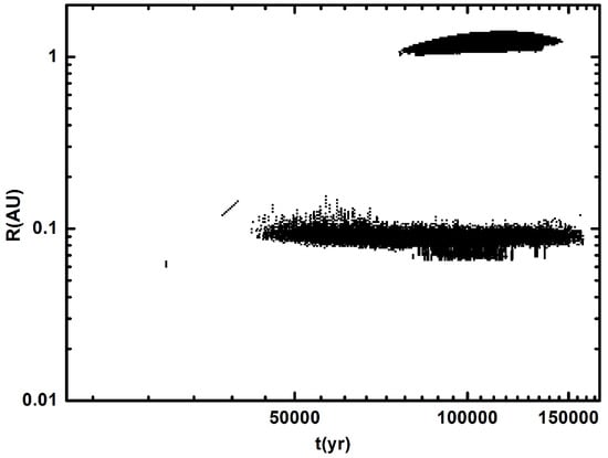
Figure 1. The recorded outburst locations (radius) in the evolution time $t$ during the early stage are displayed. Every squared point in the figure represents an outburst location (radius) in the disk at time $t$. The parameters in this figure are $\omega =2.8\times {10}^{-14}{ \mathrm{s}}^{-1}$, $T_{\mathrm{cd}}=15 \mathrm{K}$, $M_{\mathrm{cd}}=1 M_{\odot }$, and ${\alpha }_{\min }=5\times {10}^{-4}$. The radius spacing between two outburst regions is $0.963 \mathrm{AU}$.

To determine the temporal properties of outbursts at a radius in the inner disk, we need to scan the whole disk $R~0.06–5 \mathrm{AU}$, following the entire evolution time $0–1.59\times {10}^5 \mathrm{yr}$ at every radius $R$ of the disk. Then, we must check whether the judgment criterion of the outburst can be satisfied at every radius $R$ of the disk. If the judging criterion of the outburst can be satisfied at a certain radius $R$ across the whole evolution $0–1.59\times {10}^5 \mathrm{yr}$, we can then regard this radius as the outburst location. Otherwise, we must regard this radius as a non-outburst location. We used this method to determine the outburst region in the disk. In this way, we determined that there are indeed two outburst regions in the disk in Case I ($\omega =2.8\times {10}^{-14}{ \mathrm{s}}^{-1}$, $T_{\mathrm{cd}}=15 \mathrm{K}$, $M_{\mathrm{cd}}=1 M_{\odot }$, and ${\alpha }_{\min }=5\times {10}^{-4}$), and the inner Region I is $R~0.079–0.104 \mathrm{AU}$, while the outer Region II is $R~1.067–1.439 \mathrm{AU}$.

We subsequently provide the numerical results in the following. In Figure 2, we present the mass accretion rates ${\stackrel{·}{M}}_{disk}$ vs. the evolution time $t$ at the typical locations of the two outburst regions. In Figure 2a, the typical location is at $R~0.091 \mathrm{AU}$; in Figure 2b, the typical location is at $R~1.407 \mathrm{AU}$. The typical locations of 0.091 and 1.407 AU were selected as the median values of the two regions ($0.079–0.104 \mathrm{AU}$ and $1.067–1.439 \mathrm{AU}$), respectively. We found that ${\stackrel{·}{M}}_{disk}$ is high enough (${\stackrel{·}{M}}_{disk}>5\times {10}^{-5} M_{\odot }/\mathrm{yr}$) for the overall outburst.

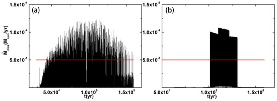
Figure 2. The mass accretion rates vs. the evolution time at the typical locations of Region I and Region II are displayed. The parameters in this figure are $\omega =2.8\times {10}^{-14}{ \mathrm{s}}^{-1}$, $T_{\mathrm{cd}}=15 \mathrm{K}$, $M_{\mathrm{cd}}=1 M_{\odot }$, and ${\alpha }_{\min }=5\times {10}^{-4}$. (a) ${\stackrel{·}{M}}_{disk}$ vs. $t$ at the location $R~0.091 \mathrm{AU}$; (b) ${\stackrel{·}{M}}_{disk}$ vs. $t$ at the location $R~1.407 \mathrm{AU}$. The black line represents ${\stackrel{·}{M}}_{disk}$, and the red line represents the critical value $5\times {10}^{-5} M_{\odot }/\mathrm{yr}$.

The lines in the two panels vibrate violently. Additionally, the outburst patterns in Region I and Region II are different. In Region I (Figure 2a), the mass accretion rate lines behave like a forest. The high (${\stackrel{·}{M}}_{disk}>5\times {10}^{-5} M_{\odot }/\mathrm{yr}$) and low states of the mass accretion alternate. In Region II (Figure 2b), the “trees” become denser. This implies that our disk model is more active, and thus the outburst may be stronger. Our disk model can provide enough energy for the outbursts.

In Figure 3, we present ${\stackrel{·}{M}}_{disk}$ vs. $t$ at $R~0.091 \mathrm{AU}$ for comparison. All the parameters are the same as in Figure 2, with the only difference being in the total evolutionary time of the disk $~3.2\times {10}^5 \mathrm{yr}$. We found that the values of ${\stackrel{·}{M}}_{disk}$ are nearly the same as in Figure 2a when we increase the total evolutionary time of the disk to $~3.2\times {10}^5 \mathrm{yr}$, and the outburst in our disk model still stops at time $~1.59\times {10}^5 \mathrm{yr}$. This means that the outbursts occur and stop at a very early stage of evolution in our disk model.

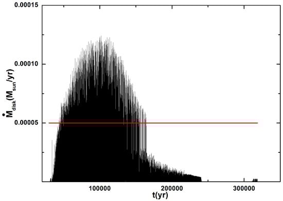
Figure 3. The mass accretion rates ${\stackrel{·}{M}}_{disk}$ vs. the evolution time $t$ at $R~0.091 \mathrm{AU}$. The other parameters are the same as in Figure 2. The only difference is the total evolutionary time of the disk, which is $~3.2\times {10}^5 \mathrm{yr}$.

In Figure 4, we present ${\alpha }_{\mathrm{MRI}}$ through the evolution at $R~0.091 \mathrm{AU}$ (a) and $R~1.407 \mathrm{AU}$ (b). The other parameters were set the same as in Figure 2. We found that the MRI operates robustly in Region I of the outburst in the early stage of evolution (${\alpha }_{\mathrm{MRI}}~0.008$), while the MRI nearly disappears in Region II of the outburst (${\alpha }_{\mathrm{MRI}}~0.001$). This is because the temperature in the inner region is high enough to cause thermal ionization, and the MRI mechanism can operate robustly in the inner region of the disk. However, in Region II of the outburst, the temperature is not high enough to cause thermal ionization, and the disk is insufficiently rarefied for cosmic ray penetration. Thus, the MRI nearly disappears in Region II of the outburst. According to Kadam et al. (2020) [6], Bae et al. (2014) [5], and Scholz et al. (2013) [39], the outbursts can mainly be caused by the following mechanisms: thermal instability, magnetorotational instability (MRI), gravitational instability (GI), the inward migration of clumps in a fragmented disk, star–disk encounters, and so on. This shows that the MRI can occur in Region I of the outburst in our disk model, while it cannot occur in Region II of the outburst.

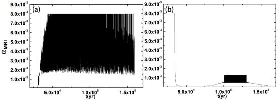
Figure 4. The viscosity due to the MRI mechanism ${\alpha }_{\mathrm{MRI}}$ vs. the evolution time $t$ at $R~0.091 \mathrm{AU}$ (a) and $R~1.407 \mathrm{AU}$ (b). The other parameters are set the same as in Figure 2.

In Figure 5, we present the time evolution of the midplane temperature $T_{\mathrm{m}}$ at $R~0.091 \mathrm{AU}$ (the black solid line) and $R~1.407 \mathrm{AU}$ (the red dashed line). We found that the temperature of the inner Region I is $~2000–3500 \mathrm{K}$, while the temperature of the outer Region II is $~1200 \mathrm{K}$. This implies that neither the inner Region I nor the outer Region II of the outburst are caused by classical thermal instability, which typically occurs at $~7000–10000 \mathrm{K}$ due to hydrogen ionization. According to Kadam et al. (2020), an instability similar to classical thermal instability can occur in the fully MRI-active disk at approximately $~1400–3500 \mathrm{K}$. This instability is caused by the steep dependence of the Rosseland opacity on the temperature. This instability is termed as “TI-1” and “TI-2” instabilities. Therefore, “TI-1” or “TI-2” instabilities can occur in the inner Region I of the outburst, while they cannot occur in the outer Region II of the outburst.

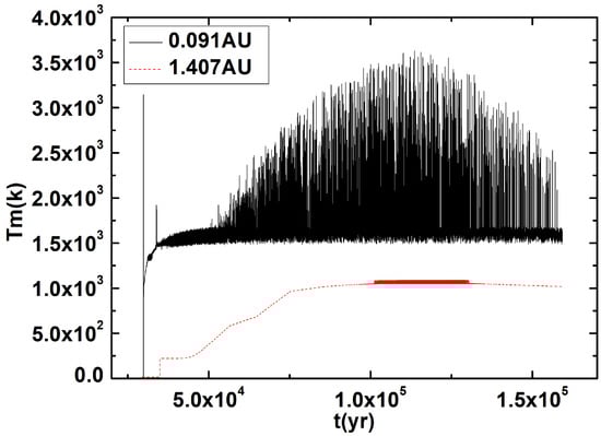
Figure 5. The time evolution of the midplane temperature $T_{\mathrm{m}}$ at $R~0.091 \mathrm{AU}$ (the black solid line) and $R~1.407 \mathrm{AU}$ (the red dashed line). The other parameters are set the same as in Figure 2.

From Figure 2, Figure 3, Figure 4 and Figure 5, we can see that many of the physical quantities exhibit sharp variations over time. This is because of the method of calculating temperature in the disk—the balance of energy. We used the immediate balance of the surface radiation flux and heating to calculate the temperature of the disk (see Equation (10)). We did not set the relaxation time for the temperature to reach balance slowly in the model. When one type of heating changes, the temperature changes immediately. This is the standard vertical thermal balance model of Bell and Lin (1994) [1]. However, in fact, there are non-vertical thermal balance heating sources in the disk, especially during the outburst event. Occasionally, some non-local energy sources (including advective heat transport and radial radiative diffusion) may dominate the internal energy flow and make the disk deviate significantly from the vertical thermal balance. Thus, the current method of temperature calculation cannot account for the non-vertical thermal balance here, and we will improve the method of temperature calculation in future work. Additionally, these sharp variations can also be partially caused by numerical error. This is due to the improper treatment of the numerical method in our model. This is the key to our future work. However, these sharp variations are not a sequence of unresolved peaks; they still have physical meanings. This is because the duration of the outburst events is much longer than the time step of the model. The duration of the outburst events at $R~0.091 \mathrm{AU}$ is around 0.1 yr, while the duration of the outburst events at $R~1.407 \mathrm{AU}$ is a few yrs. The time step of the model is about 0.001 yr. Therefore, sharp variations are not artefacts, they are physical effects.

3.2. The Physical Reason for the Two Regions

From the above discussions, we can conclude that the outburst in Region I is caused by MRI and the “TI-1” or “TI-2” instabilities, rather than GI. Additionally, the outburst in Region II is not caused by thermal instability, MRI, or GI.

From Figure 4, we can see that Region I is dominated by MRI, while Region II is not dominated by MRI. From Figure 5, we can see that the classical thermal instability does not operate in Region I, while “TI-1” or “TI-2” instabilities can operate in Region I ($~2000–3500 \mathrm{K}$). Therefore, we can see that both MRI and the “TI-1” or “TI-2” instabilities can operate in Region I; furthermore, our analysis suggests that both MRI and the “TI-1” or “TI-2” instabilities dominate in Region I.

Concerning Region II ($R~1.067-1.439 \mathrm{AU}$), more analysis is needed. To determine the physical reasons for Region II, we analyzed all the quantities in this region, such as the surface density $\mathrm{\Sigma }$, ${\kappa }_R$, $T_{\mathrm{m}}$, $\alpha$, and so on. We found no abnormities in these quantities in Region II, except ${\kappa }_R$. In Figure 6 and Figure 7, we present the radial distribution of ${\kappa }_R$ at different time instances $t$. The time step is also $6.37 \mathrm{yr}$, and the parameters are set the same as in Figure 2. We found that ${\kappa }_R$ vibrates violently in Region II. The Rosseland mean opacity influences the viscous heating, the radiative diffusion, and the radiation, and our analysis suggests that Region II is dominated by the vibration of ${\kappa }_R$. Moreover, from Figure 8, when we increase the ${\alpha }_{\min }$ parameter to $1\times {10}^{-3}$, Region II disappears. In conclusion, our analysis suggests that Region II is dominated by, or is largely related to, the ${\kappa }_R$ and ${\alpha }_{\min }$ parameters.

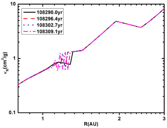
Figure 6. The radial distribution of ${\kappa }_R$ at different evolution time instances $t$. The time step is $6.37 \mathrm{yr}$ from the time instance $t=\mathrm{108,290.0} \mathrm{yr}$. The model parameters in this figure are set the same as in Figure 2.

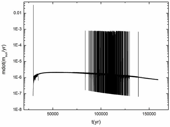
Figure 7. The mass accretion rates ${\stackrel{·}{M}}_{disk}$ vs. the evolution time $t$ at the inner boundary $R~0.06 \mathrm{AU}$. The parameters are set the same as in Figure 2.

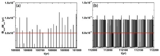
Figure 8. ${\stackrel{·}{M}}_{disk}$ in short time intervals at $R~0.091 \mathrm{AU}$ (a) and $R~1.407 \mathrm{AU}$ (b). The time intervals for panels (a,b) are $\mathrm{100,500}-\mathrm{101,000} \mathrm{yr}$ and $\mathrm{112,000}-\mathrm{112,200} \mathrm{yr}$, respectively. The other parameters are set the same as in Figure 2.

To demonstrate that the structure in our disk model is not a numerical artefact or an effect with trivial explanation/consequences, and to justify the code of our disk model, we tested the viscous evolution of an initially thin ring, e.g., the inner boundary $0.06 \mathrm{AU}$ and the neighboring rings $0.061 \mathrm{AU}$, $0.063 \mathrm{AU}$. We found that the surface density of the inner boundary $0.06 \mathrm{AU}$ remains zero, and $T_{\mathrm{m}}$ remains $15 \mathrm{K}$ the whole time. This result is as expected, because this is the inner boundary condition we set in our disk model. For the neighboring rings $0.061 \mathrm{AU}$, $0.063 \mathrm{AU}$, we found that $\mathrm{\Sigma }$ first increases to about ${\mathrm{10,000} \mathrm{gcm}}^{-2}$, and then it nearly remains constant before the mass influx from the cloud core stops. The temperature also behaves similarly. These results are also as expected, because as the mass influx from the parent cloud core reaches the disk, the inner disk starts to form and the material mass increases more and more. With the continuous mass influx onto the inner disk, the material in the inner disk also accretes inward to the central protostar; thus, the surface density remains nearly constant. In conclusion, we tested the viscous evolution of an initially thin ring, finding that the code behaves as expected. Therefore, the results can be trusted.

In Figure 7, we present the mass accretion rates during the evolution time at the inner boundary $R~0.06 \mathrm{AU}$ for details. The parameters are set the same as in Figure 2. We can see that the mass accretion rates are very large at the inner boundary. The mass accretion rates first have an impulse value $~0.03 M_{\odot }/\mathrm{yr}$, but it is transient. And then, they have sharp variations with high states and low states; this is inevitable in our model because of the method of calculating temperature. The high states have the mass accretion rates $~1\times {10}^{-3} M_{\odot }/\mathrm{yr}$, and the average value of the mass accretion rates is $~1\times {10}^{-6} M_{\odot }/\mathrm{yr}$. Additionally, we also checked the other quantities at the inner boundary, such as the surface density, temperature, viscosity, and H/R. We see that the surface density remains zero, and $T_{\mathrm{m}}$ remains $15 \mathrm{K}$ the whole time; these are the inner boundary conditions we set. The viscosity $\alpha$ has the value of $0.008$; this is due to the MRI. The H/R has the value $~0.006$, and this shows that the scale height H is small at the inner boundary.

Our paper focuses on the outburst properties of the inner region. In our disk model, although the mass accretion rate can be compared with that of FU Orionis outbursts, the duration timescale of a single typical FU Orionis outburst cannot be compared with the observations. In our disk model, the duration timescale of a single outburst is about a few yrs or even shorter, and the outburst is seen to be more transient. This may still be of interest, because other observational studies [40] have also found many non-typical FU Orionis outbursts and EXor outbursts. These non-typical FU Orionis and EXor outbursts all have short duration timescales (tens of yrs to a few $0.1 \mathrm{yr}$). Although the duration timescales of the outbursts in our disk model are inconsistent with the typical FU Orionis outbursts, we can still account for the non-typical FU Orionis and EXor outbursts. For the purpose of developing a disk model to compare with the observations on all the outbursts (including the typical or non-typical FU Orionis and EXor outbursts) completely, more research is needed in future studies.

In Figure 8, for more detailed insight, we present a sketch of ${\stackrel{·}{M}}_{disk}$ in short time intervals at $R~0.091 \mathrm{AU}$ (a) and $R~1.407 \mathrm{AU}$ (b). The time intervals for panels (a) and (b) are $\mathrm{100,500}–\mathrm{101,000} \mathrm{yr}$ and $\mathrm{112,000}–\mathrm{112,200} \mathrm{yr}$, respectively. The other parameters are set the same as in Figure 2. We can see that the outburst in Region I in the $500 \mathrm{yr}$ time interval is discrete in time, not continuous. The outburst in Region II in the $200 \mathrm{yr}$ time interval is also discrete in time, but much denser.

According to the observations of Audard et al. (2014) [40], a single outburst lasts about 100 yrs and a typical star undergoes 10 such bursts. The timescale of a typical single outburst is inconsistent with that of our disk model. The duration timescale of a single outburst in our disk model is a few years or shorter, and the outburst in our disk model is more transient. There is indeed a large difference between the outbursts in our disk model and the observations on a typical outburst. Our analysis suggests that this difference is caused by the different codes of the disk model or the different numerical methods. However, observations on FU Orionis outbursts [40] also found many non-typical FU Orionis and EXor outbursts. These non-typical FU Orionis outbursts and EXor outbursts are all transient and have short duration timescales (tens of years to a few $0.1 \mathrm{yr}$). Additionally, they found that there is a clear overlap in the mass accretion rate between the FU Orionis outbursts and EXor outbursts. Whether or not the FU Orionis and EXor outbursts should be classified into two distinct classes is still an open question. A proposal has been put forward that suggests that the distribution of FU Orionis and EXor outbursts is more like a continuum, rather than two distinct classes. Although our numerical results for the outbursts (duration timescale and frequency) are incompatible with a typical FU outburst, the numerical results for outbursts in our disk model can seemingly account for the observational data on non-typical FU Orionis and EXor outbursts in magnitude. They are all transient and have short duration timescales (tens of years to a few $0.1 \mathrm{yr}$).

3.3. The Varying Parameters Model

We subsequently ran the code with different parameters and tried to find links to the properties of the molecular cloud core and ${\alpha }_{\min }$ parameter. Firstly, we increased the ${\alpha }_{\min }$ parameter to $1\times {10}^{-3}$, while the other parameters were the same as in Case I. We found that Region II of the outburst disappears, and only Region I of the outburst exists. Region I is located at $R~0.079–0.107 \mathrm{AU}$, almost the same as in Case I. In Figure 9, we present ${\stackrel{·}{M}}_{disk}$ vs. t with ${\alpha }_{\min }=1\times {10}^{-3}$ at $R~0.091 \mathrm{AU}$. The other parameters are set the same as in Figure 2. We can see that the behavior of ${\stackrel{·}{M}}_{disk}$ is similar to that in Case I. However, the maximum mass accretion rate ${\stackrel{·}{M}}_{disk}$ increases slightly compared to Case I, and this is because the ${\alpha }_{\min }$ parameter controls the viscous evolution when both the MRI and GI cannot operate. In the innermost regions of the disk, MRI can operate all the time due to thermal ionization. Thus, the increased ${\alpha }_{\min }$ parameter has slight (but not zero) influence on the mass accretion rate behavior in the innermost regions. The major difference is that Region II of the outburst disappears. This implies that the physical reasons for the outburst in Region II (neither MRI, GI, nor thermal instability) are dominated by, or largely related to, the ${\kappa }_R$ and ${\alpha }_{\min }$ parameters.

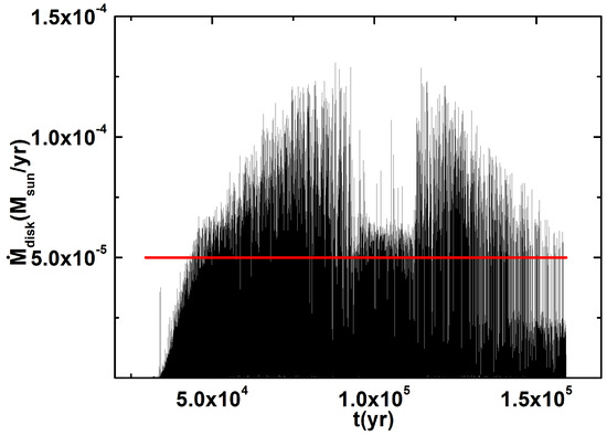
Figure 9. ${\stackrel{·}{M}}_{disk}$ vs. $t$ at $R~0.091 \mathrm{AU}$ with ${\alpha }_{\min }=1\times {10}^{-3}$. The other parameters are set the same as in Figure 2.

Finally, we changed $M_{\mathrm{cd}}$ to $0.5 M_{\odot }$ and calculated the mass accretion rate during the early evolution. The two regions of the outburst are $R~0.082–0.097 \mathrm{AU}$ and $R~1.312–1.439 \mathrm{AU}$. In Figure 10, we present ${\stackrel{·}{M}}_{disk}$ vs. $t$ at the typical locations of the outburst regions with $M_{\mathrm{cd}}=0.5 M_{\odot }$ (Case II). The other parameters are set the same as in Figure 2. The typical locations of the outburst regions are $R~0.091 \mathrm{AU}$ (Figure 10a) and $R~1.407 \mathrm{AU}$ (Figure 10b). We found that the mass accretion rate in the low-mass case is similar to that in Case I (Figure 2), but with a small difference. This is because the gravitational collapse of the molecular cloud core has an inside-out pattern; thus, the early evolution of the protoplanetary disk + protostar system with different masses of the molecular cloud core has a self-similar pattern. The major difference in the evolution occurs in the T Tauri and the dissipation phases, not the early phase (the embedded phase). This implies that $M_{\mathrm{cd}}$ has a slight influence on the outburst properties in the early evolution of the protoplanetary disk.

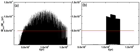
Figure 10. ${\stackrel{·}{M}}_{disk}$ vs. $t$ at the typical locations of the outburst regions with $M_{\mathrm{cd}}=0.5 M_{\odot }$. (a) The location is at $R~0.091 \mathrm{AU}$; (b) the location is at $R~1.407 \mathrm{AU}$. The other parameters are set the same as in Figure 2.

4. Conclusions and Discussion

The mass accretion properties in the inner regions of the protoplanetary disk [10] were investigated in this paper. The accretion rate satisfies the judgment criterion (high) at certain time points and locations. However, the outburst points are dense enough in time and space; thus, ${\stackrel{·}{M}}_{disk}$ in inner regions of our disk model can statistically satisfy the judgment criterion and provide a large amount of energy for the overall outburst. We ran the code of the evolutionary disk model with different parameters of the molecular cloud core ($\omega$, $T_{\mathrm{cd}}$, and $M_{\mathrm{cd}}$) and the ${\alpha }_{\min }$ parameter, aiming to find some correlations between the properties of the molecular cloud core and the outburst events. We found that the occurrence of outburst events has a weak correlation with the properties of the molecular cloud core; however, it has a strong correlation with the ${\kappa }_R$ and ${\alpha }_{\min }$ parameters.

From our work, we obtained the following conclusions:

(1) In Case I ($\omega =2.8\times {10}^{-14}{ \mathrm{s}}^{-1}$, $T_{\mathrm{cd}}=15 \mathrm{K}$, $M_{\mathrm{cd}}=1 M_{\odot }$, and ${\alpha }_{\min }=5\times {10}^{-4}$), there are two outburst regions: Region I is located at $R~0.082–0.097 \mathrm{AU}$, while Region II is located at $R~1.312–1.439 \mathrm{AU}$. The mass accretion rate in the inner regions of our disk model can statistically satisfy the judgment criterion and provide a large amount of energy for the overall outburst.

(2) The physical reasons for the inner Region I are the MRI and “TI-1” or “TI-2” instabilities, rather than GI. Additionally, the outer Region II is not caused by thermal instability, MRI, or GI. Our analysis suggests that the outer Region II is dominated by, or largely related to, the ${\kappa }_R$ and ${\alpha }_{\min }$ parameters.

(3) As the ${\alpha }_{\min }$ parameter increases to $1\times {10}^{-3}$, the mass accretion rate of the inner Region I is slightly increased, and Region II of the outburst disappears. This is because the ${\alpha }_{\min }$ parameter controls the viscous evolution when both MRI and GI cannot operate. However, in the innermost regions of the disk, the MRI can operate all the time due to thermal ionization. Thus, the increased ${\alpha }_{\min }$ parameter has slight (but not zero) influence on the mass accretion rate in the inner Region I, but it has a significant influence on the outer Region II.

(4) As $M_{\mathrm{cd}}$ decreases to $0.5 M_{\odot }$, ${\stackrel{·}{M}}_{disk}$ is almost the same as in Case I. This is because the gravitational collapse of the molecular cloud core has an inside-out (self-similar) pattern; thus, the early formation and evolution of the protoplanetary disk in the high-mass case is the same as in the low-mass case. Therefore, the mass of the molecular cloud core has a slight influence on the outburst events in our disk model.

References

- Bell, K.R.; Lin, D.N.C. Using FU Orionis Outbursts to Constrain Self-Regulated Protostellar Disk Models. Astrophys. J. 1994, 427, 987–1004. [Google Scholar] [CrossRef]
- Vorobyov, E.I.; Basu, S. The Burst Mode of Accretion and Disk Fragmentation in the Early Embedded Stages of Star Formation. Astrophys. J. 2010, 719, 1896–1911. [Google Scholar] [CrossRef]
- Fleming, T.; Stone, J.M. Local Magnetohydrodynamic Models of Layered Accretion Disks. Astrophys. J. 2003, 585, 908–920. [Google Scholar] [CrossRef]
- Chambers, J.E. Planet Formation with Migration. Astrophys. J. 2006, 652, L133–L136. [Google Scholar] [CrossRef][Green Version]
- Bae, J.; Hartmann, L.; Zhu, Z.; Nelson, R.P. Accretion Outbursts in Self-Gravitating Protoplanetary Disks. Astrophys. J. 2014, 795, 61–75. [Google Scholar] [CrossRef]
- Kadam, K.; Vorobyov, E.; Regály, Z.; Kóspál, Á.; Ábrahám, P. Outbursts in Global Protoplanetary Disk Simulations. Astrophys. J. 2020, 895, 41–56. [Google Scholar] [CrossRef]
- Forgan, D.; Rice, K. Stellar Encounters in the context of Outburst Phenomena. Mon. Not. R. Astron. Soc. 2010, 402, 1349–1356. [Google Scholar] [CrossRef]
- Bonnell, I.; Bastien, P. A Binary Origin for FU Orionis Stars. Astrophys. J. 1992, 401, L31. [Google Scholar] [CrossRef]
- Lodato, G.; Clarke, C.J. Massive Planets in FU Orionis Discs: Implications for Thermal Instability Models. Mon. Not. R. Astron. Soc. 2004, 353, 841–854. [Google Scholar] [CrossRef]
- Liu, C.J.; Yao, Z.; Li, H.N.; Wang, H.S. The Evolution of the Protoplanetary Disk with Mass Influx from a Molecular Cloud core and the Photoevaporation Winds. New Astron. 2018, 58, 72–83. [Google Scholar] [CrossRef]
- Jin, L.; Li, M. Diversity of Extrasolar Planets and Diversity of molecular cloud cores. I. Semimajor Axes. Astrophys. J. 2014, 783, 37–55. [Google Scholar] [CrossRef]
- Nakamoto, T.; Nakagawa, Y. Formation, Early Evolution, and Gravitational Stability of Protoplanetary Disks. Astrophys. J. 1994, 421, 640. [Google Scholar]
- Alexander, R.D.; Clarke, C.J.; Pringle, J.E. Photoevaporation of Protoplanetary Discs.-I. Hydrodynamic Models. Mon. Not. R. Astron. Soc. 2006, 369, 216. [Google Scholar] [CrossRef]
- Alexander, R.D.; Clarke, C.J.; Pringle, J.E. Photoevaporation of Protoplanetary Discs.-II. Evolutionary Models and Observable Properties. Mon. Not. R. Astron. Soc. 2006, 369, 229. [Google Scholar] [CrossRef]
- Kratter, K.M.; Matzner, C.D.; Krumholz, M.R. Global Models for the Evolution of Embedded, Accreting Protostellar Disks. Astrophys. J. 2008, 681, 375. [Google Scholar] [CrossRef]
- Laughlin, G.; Bodenheimer, P. Nonaxisymmetric Evolution in Protostellar Disks. Astrophys. J. 1994, 436, 335. [Google Scholar] [CrossRef]
- Laughlin, G.; Rozyczka, M. The Effect of Gravitational Instabilities on Protostellar Disks. Astrophys. J. 1996, 456, 279. [Google Scholar] [CrossRef]
- Umebayashi, T. The Densities of Charged particles in very dense Interstellar Clouds. Prog. Theor. Phys. 1983, 69, 480. [Google Scholar] [CrossRef]
- Zhu, Z.; Hartmann, L.; Nelson, R.P.; Gammie, C.F. Challenges in Forming Planets by Gravitational Instability: Disk Irradiation and Clump Migration, Accretion, and Tidal Destruction. Astrophys. J. 2012, 746, 110. [Google Scholar] [CrossRef]
- McKee, C.F.; Ostriker, E.C. Theory of Star Formation. Annu. Rev. Astron. Astrophys. 2007, 45, 565. [Google Scholar] [CrossRef]
- Goodman, A.A.; Benson, P.J.; Fuller, G.A.; Myers, P.C. Dense Cores in Dark Clouds. VIII. Velocity Gradients. Astrophys. J. 1993, 406, 528. [Google Scholar]
- Caselli, P.; Benson, P.J.; Myers, P.C.; Tafalla, M. Dense Cores in Dark Clouds. XIV. N2H+ (1-0) Maps of Dense cloud Cores. Astrophys. J. 2002, 572, 238. [Google Scholar] [CrossRef]
- Shu, F.H. Self-similar collapse of Isothermal spheres and Star Formation. Astrophys. J. 1977, 214, 488. [Google Scholar] [CrossRef]
- Jijina, J.; Myers, P.C.; Adams, F.C. Dense Cores Mapped in Ammonia: A Database. Astrophys. J. Suppl. Ser. 1999, 125, 161. [Google Scholar] [CrossRef]
- Motte, F.; Andre, P.; Neri, R. The Initial Conditions of Star Formation in the rho Ophiuchi Main Cloud: Wild-field millimeter continuum mapping. Astron. Astrophys. 1998, 336, 150. [Google Scholar]
- Shakura, N.I.; Sunyaev, R.A. Black Holes in Binary Systems. Observational Appearance. Astron. Astrophys. 1973, 24, 337. [Google Scholar]
- Jin, L.; Sui, N. The Evolution of the Solar Nebula. I. Evolution of the Global Properties and Planet Masses. Astrophys. J. 2010, 710, 1179. [Google Scholar] [CrossRef]
- Fukue, J. Radiative Transfer in Protoplanetary Disks under Irradiation by the Protostar. Prog. Theor. Exp. Phys. 2013, 5, 053E02. [Google Scholar] [CrossRef][Green Version]
- Balbus, S.A.; Hawley, J.F. A Powerful Local Shear Instability in Weakly Magnetized Disks. I. Linear Analysis. Astrophys. J. 1991, 376, 214. [Google Scholar] [CrossRef]
- Gammie, C.F. Layered Accretion in T Tauri Disks. Astrophys. J. 1996, 457, 355. [Google Scholar] [CrossRef]
- Lodato, G.; Rice, W.K.M. Testing the Locality of Transport in Self-Gravitating Discs -II. The Massive Disc Case. Mon. Not. R. Astron. Soc. 2005, 358, 1489. [Google Scholar] [CrossRef]
- Forgan, D.; Rice, K.; Cossins, P.; Lodato, G. The Nature of Angular Momentum Transport in Radiative Self-Gravitating Protostellar Discs. Mon. Not. R. Astron. Soc. 2011, 410, 994. [Google Scholar] [CrossRef]
- Toomre, A. On the Gravitational Instability of a Disk of Stars. Astrophys. J. 1964, 139, 1217. [Google Scholar] [CrossRef]
- Dubrulle, B. Differential Rotation as a Source of Angular Momentum Transfer in the solar nebula. Icarus 1993, 106, 59. [Google Scholar] [CrossRef]
- Klahr, H.H.; Bodenheimer, P. Turbulence in Accretion Disks: Vorticity Generation and Angular Momentum Transport via the Global Baroclinic Instability. Astrophys. J. 2003, 582, 869. [Google Scholar] [CrossRef]
- Richard, D. On non-linear hydrodynamic instability and enhanced transport in differentially rotating flows. Astron. Astrophys. 2003, 408, 409. [Google Scholar] [CrossRef][Green Version]
- Dubrulle, B.; Marié, L.; Normand, C.; Richard, D.; Hersant, F.; Zahn, J.P. An hydrodynamic shear instability in stratified disks. Astron. Astrophys. 2005, 429, 1. [Google Scholar]
- Clarke, C.J.; Lin DN, C. Pre-conditions for disc generated FU Orionis outbursts. Mon. Not. R. Astron. Soc. 1990, 242, 439. [Google Scholar] [CrossRef]
- Scholz, A.; Froebrich, D.; Wood, K. A systematic survey for eruptive young stellar objects using mid-infrared photometry. Mon. Not. R. Astron. Soc. 2013, 430, 2910. [Google Scholar] [CrossRef]
- Audard, M.; Ábrahám, P.; Dunham, M.M.; Green, J.D.; Grosso, N.; Hamaguchi, K.; Kastner, J.H.; Kóspál, A.; Lodato, G.; Romanova, M.M.; et al. Epesodic Accretion in Young Stars. In Protostars and Planets VI; Beuther, H., Klessen, R.S., Dullemond, C.P., Henning, T.K., Eds.; University of Arizona Press: Tucson, AZ, USA, 2014; p. 387. [Google Scholar]
Disclaimer/Publisher’s Note: The statements, opinions and data contained in all publications are solely those of the individual author(s) and contributor(s) and not of MDPI and/or the editor(s). MDPI and/or the editor(s) disclaim responsibility for any injury to people or property resulting from any ideas, methods, instructions or products referred to in the content. |
© 2024 by the authors. Licensee MDPI, Basel, Switzerland. This article is an open access article distributed under the terms and conditions of the Creative Commons Attribution (CC BY) license (https://creativecommons.org/licenses/by/4.0/).