Abstract
The TESS light curve of the silicon Ap star MX TrA was modeled using the observational surface distribution of silicon, iron, helium, and chromium obtained previously with the Doppler Imaging technique. The theoretical light curve was calculated using a grid of synthetic fluxes from line-by-line stellar atmosphere models with individual chemical abundances. The observational TESS light curve was fitted by a synthetic one with an accuracy better than 0.001 mag. The influence of Si and Fe abundance stratification on the amplitude of variability was estimated. Also, the wavelength dependence of the photometric amplitude and phase of the maximum light was modeled showing the typical Ap Si star behavior with increased amplitude and anti-phase variability in far ultraviolet caused by the flux redistribution.
PACS:
95.75.-z; 95.75.De; 97.10.Ex; 97.10.Kc; 97.30.Fi
1. Introduction
Chemically peculiar magnetic Ap/Bp stars are characterized by a strongly inhomogeneous distribution of chemical elements in their atmospheres, both over the surface and in depth. Driven by selective atomic diffusion [1] these inhomogeneities follow the surface geometry of the magnetic field and form the horizontal abundance gradients-the chemical spots with increased or decreased abundance of certain elements up to a few dex (in logarithmic scale) relative to the Sun. Due to the line blanketing the opacity differs significantly within spots and quiet photosphere that affects the emergent flux. The axial rotation of a spotted star leads to periodic brightness variability. This is the key ingredient of the “oblique rotator” model [2], which successfully explains the variability in Ap/Bp stars.
Recent developments in the computation of model atmospheres with individual chemical composition [3] as well as observational Doppler imaging (DI) technique see, e.g., [4,5] for review, has led to major advances in the interpretation of observations of Ap/Bp stars. A study of model atmosphere computed with line-by-line opacity treatment Khan and Shulyak [6] showed that individual abundance patterns result in changing the atmospheric structure. The temperature and pressure distribution, and modification of the spectral energy distribution (SED). Elements such as silicon, iron and chromium which are often significantly overabundant in the line-forming region of Ap/Bp atmospheres, were found to be the principal contributors to opacity. In particular, Si plays an exceptional role both in line and continuum opacities in the ultraviolet (UV) region [7] that leads to the flux redistribution between far- ( Å) and near-UV as well as the visible spectral region. In turn, this effect manifests in distinct photometric behavior of silicon Ap/Bp stars depending on the bandpass. The combination of these theoretical and numerical advances with the capability of surface mapping with DI offers a direct opportunity for robust modeling and interpretation of the spectral and photometric variability of Ap/Bp stars.
In a series of papers [8,9,10,11] the light curves of Ap/Bp stars were modeled using the surface distributions of elements obtained by the DI method. As a result, a sufficiently good agreement between the synthetic light curves and the observed ones was obtained, proving surface elemental inhomogeneity as the reason for the light changes in investigated stars. Also, in agreement with theoretical predictions, the key contribution of spots with silicon, iron, and chromium overabundance to the rotational light modulation was confirmed.
Nevertheless, the problem is still relevant due to the growing number of precise high-cadence photometric observations from the spacecraft Kepler/K2 [12], BRITE [13], TESS [14], etc., and accurate representation of the light curves of Ap/Bp stars may shed new light on some new effects. Thus, the large diversity of the surface distributions of elements in Ap/Bp stars will allow us to disentangle the contribution of individual elements to the total photometric variation and compare it with theoretical expectations. The impact of effects such as deviation from the local thermodynamic equilibrium (LTE) and vertical abundance gradients (stratification) on the flux variations of Ap/Bp stars is not completely explored and its accounting will probably improve the accuracy of the fit to the observations.
The aim of the present work is the quantitative investigation of the effect of inhomogeneous surface abundance distribution of most peculiar elements in Ap star MX TrA on its photometric variability. MX TrA (HD 152564) is a bright southern Ap star that belongs to the silicon subgroup of this class and demonstrates pronounced photometric variability [15]. Based on the high-resolution phase-resolved spectroscopy of MX TrA Potravnov et al. [16] determined the fundamental and atmospheric parameters (the effective temperature = 11,950 ± 200 K, the surface gravity log g = 3.6 ± 0.2, the microturbulent velocity = 0.0 km/s, the macroturbulent velocity = 0.0 km/s, the projection of the rotational velocity sin i = 69 ± 2 km/s, the mass = 2.1, the radius = 3.8), abundances of 12 ions of nine elements and also mapped the surface abundance distributions for Si, He, Fe, Mg, and O using DI. Later, Potravnov and Ryabchikova [17] obtained Cr maps with the same DI technique. Analysis of high-precision photometric data from the TESS spacecraft revealed a period of days, which, together with the values of the projectional rotational velocity sin i and the radius of the star R, gives the value of the orbital inclination i . The phased light curve has an amplitude of about 0.03 m and a quasi-sinusoidal shape, which reflects the modulation by the rotation of the spotted star. A pronounced rotationally modulated variability due to a highly inhomogeneous surface distribution of elements and the expected presence of vertical stratification of silicon and iron makes MX TrA an exceptionally suitable object for investigation in the context of the problem above.
The present work is based on the Doppler Imaging results obtained in Potravnov et al. [16], Potravnov and Ryabchikova [17] and focuses on the modeling of the light curve of MX TrA. The paper is organized as follows: Section 2 provides data on the photometric observations of MX TrA and surface abundance maps we used. Section 3 describes the modeling technique, calculations of the surface intensity map and synthetic light curve, Section 4 describes the results and comparison with observations. In Section 5 we present our conclusions.
2. Observational Data
For construction of the light curve of MX TrA we used the photometric observations obtained by the TESS mission during Cycle 3 in Sector 39 (from 27 May 2021 to 24 June 2021) and comprising about 20,000 measurements with a 120-s cadence in total. We used the photometry obtained during this cycle as being closest to the main period of the spectroscopic observations used for Doppler Imaging in Potravnov et al. [16]. Given the good representation of the MX TrA light curve from season to season, these observations are reliable for our main purpose of accessing the general shape and amplitude of the light curve. The data were retrieved through the Mikulski Archive for Space Telescopes1 (MAST) portal automatically processed with the Science Processing Operations Center (SPOC) software package [18]. The processed SPOC light curve provides two types of fluxes: SAP (Simple Aperture Photometry) flux and PDCSAP (Pre-search Data Conditioning SAP) flux with removed long-term trends. In the particular case of MX TrA photometry in Sector 39 PDCSAP fluxes after removing an offset appeared to be almost identical to the SAP fluxes but noisier, hence we used the latter for magnitudes conversion. The SAP fluxes were converted to the TESS magnitude scale which is close to the Cousins filter using the formula , taken from the project documentation2. The phased light curve of MX TrA was built using an ephemeris JD(max.light) = from Potravnov et al. [16]. It should be noted that the light curve of MX TrA is slightly asymmetric, so the initial epoch in the ephemeris was determined from the center of gravity of the maximum. This explains a small negative shift relative to zero of the points with maximal brightness in the phased light curve.
We also used surface distribution maps of four elements: He, Si, Fe from Potravnov et al. [16] and Cr from Potravnov and Ryabchikova [17] for calculations of the synthetic light curves. These maps with a resolution of about on the equator were obtained with the DI technique based on a spectroscopic time series from the 10-m South African Large Telescope (SALT). Details of the spectroscopic observations and Doppler Imaging procedure are given in the papers cited above. For chromium, Potravnov and Ryabchikova [17] provides two versions of the maps with slightly different abundance scales, depending on the set of lines they used. We explore both of them in an attempt for the best representation of the observed light curve (see below).
3. Modeling of Light Curve
Our approach to light curve modeling is based on the following fundamental steps:
- Construction of a surface intensity map. For this purpose, the specific intensities in the elements of the surface grid are calculated with the individual abundances from the Doppler maps.
- Disk integration of specific intensities for all rotational phases. Convolution of the integrated flux at each phase with the bandpass of the chosen filter allows us to compare the calculated synthetic light curve with the observed one.
Details are given in the subsections below.
3.1. Construction of Intensity Map
In the first step, a grid of stellar atmosphere models was calculated with the LLmodels code [3] taking into account the individual chemical composition. The stellar parameters of MX TrA ( = 11,950 ± 200 K, log g = 3.6 ± 0.2) and the mean elemental abundances were adopted from Potravnov et al. [16]. The abundances of silicon, iron, helium, and chromium were varied within the limits inferred from Doppler maps (Figure 1). The maps are 544 × 272 pixels in size, which corresponds to an equidistant step of about 0.66° in latitude and longitude. The final grid consists of 256 atmosphere models calculated for all possible combinations of abundances in the ranges of = [−4.50 … −2.30] = [−4.70 … −3.70], = [−2.11 … −1.61], and = [−6.50 … −4.10], where abundances are expressed through the ratio the number density of element X to the total number density . The abundance of other elements remained unchanged. The synthetic SEDs were computed simultaneously with the atmosphere models. Using the response curve of the TESS imaging receiver [14] we calculated the flux and intensity of radiation from the 1 cm2 of stellar surface. The calculated intensities in the TESS magnitude scale were combined into a grid with the gradients significantly smoothed out in the logarithmic scale. For each point in the surface map, the specific intensity was calculated using the grid interpolation and taking into account the local abundances of Si, Fe, He, and Cr. Thus, an intensity map was constructed in the bandpass of the TESS image receiver. The ratio of the minimum and maximum intensities was about 0.93. This map scaled to the maximum value is shown in Figure 2. By its appearance, the intensity map better resembles the silicon distribution map. This was expected, since silicon makes the most significant contribution to the absorption coefficient, especially in the UV range. Due to energy redistribution in the stellar spectrum, strong absorption in the UV leads to an increase in flux in the visible range. Therefore, dark spots with an overabundance of silicon in the Doppler map appear bright in the intensity map.
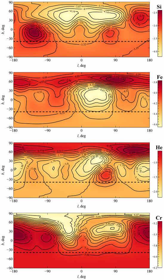
Figure 1.
Maps of the distribution of silicon, iron, helium, and chromium (sequentially from top to bottom) on the surface of the star MX TrA. The dashed line marks the lower boundary of the visible part of the surface due to the tilt of the rotation axis.
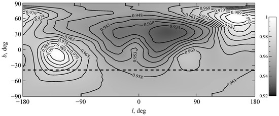
Figure 2.
Map of the relative intensity distribution in the TESS image receiver bandpass. The maximum intensity value is taken as unit.
3.2. Synthetic Magnitudes and Light Curve
The intensity map in rectangular coordinates was further transformed into a spherical one in orthographic projection taking into account inclination of the rotation axis i = 51° [16].
The apparent intensity of an arbitrary surface element (“point” in the map) with coordinates and intensity towards the observer is
where , is the vertex angle between the direction from the center of the star toward the observer and a point on the stellar surface with coordinates ; and are limb darkening coefficients; is the area of surface element on the sphere.
Limb darkening coefficients for quadratic law were calculated from the emergent radiation intensities convolved with TESS bandpass for seven values of using the Levenberg–Marquardt method [19,20] to approximate function
The calculations were made for a stellar atmosphere model with average abundances of Si, Fe, He, and Cr. The impact of individual chemical composition on the limb darkening coefficients is small and does not exceed 0.1–0.2%.
The radiation flux in the bandpass of the TESS image receiver is obtained by integrating the contribution of all points over the visible hemisphere of the star (). The synthetic magnitude is
The magnitude zero point here is equal to zero because it was already taken into account when calculating the specific intensities in magnitude scale to create the grid.
The magnitude refers to the average radiation flux from an area of 1 cm2 on the stellar surface. The apparent magnitude was calculated as
Here, is the angular diameter of the star in as. We neglect interstellar extinction due to its smallness [16].
The angular diameter as was calculated from the difference between the observed average magnitude over the rotation period and the synthetic one :
By combining this angular diameter with the distance to the star of 191 ± 9 pc obtained from inversion of Gaia DR3 parallax ( as) [21], the radius of MX TrA was obtained and found to be in good agreement with spectroscopic determination by Potravnov et al. [16].
The synthetic light curve in units was computed with Equation (4) for the full set of rotational phases and is presented in Figure 3 together with the TESS observations.
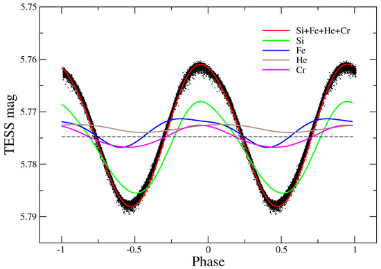
Figure 3.
Comparison of the observed light curve of MX TrA with the theoretical ones. Each synthetic curve is calculated accounting for the inhomogeneous surface abundance distribution of element(s). The dashed line indicates the theoretical magnitude calculated for uniform surface abundance distribution with average values of elemental abundances.
4. Results and Discussion
4.1. Synthetic Light Curve
Figure 3 represents theoretical light curves accounting for the individual contribution of each considered element and the total curve with the cumulative impact of all elements in comparison with the observed TESS light curve. The observed light curve has a quasi-sinusoidal shape with a more gradual descending lag. One can see from the figure that the total synthetic light curve perfectly matches the observations in terms of both amplitude and shape. Considering the individual contribution of elements, silicon has the largest one, about 64%, to the amplitude of the light variation. The contributions at the phases of maximum and minimum are different due to the inhomogeneous distribution of silicon spots over the stellar surface. That is why the light curve due to silicon surface abundance variations is asymmetrical relative to the zero phase. This asymmetry is also manifested in the shape of the observed TESS light curve as the bar near phase . A systematic error in Si abundance of the order of ±0.2 dex, which is typical in abundance analysis, results in an amplitude difference of order 0.005 mag. The amplitude reduces with silicon abundance decreases and increases with silicon in excess. The next largest contributor to brightness variations is chromium with the value of relative amplitude about 22%. Iron has an amplitude of about 20% of the total, but the light curve is shifted by phase which is consistent with the longitudinal position of the most contrast Fe spot from DI. Therefore, Fe provides a somewhat lower contribution to the total, about 17%. Helium is responsible for the smallest changes in magnitudes. A feature in the TESS light curve at phase of 0.1 is fitted well by Si, Fe, and He but with a somewhat reduced amplitude. Accounting for the contribution of chromium matches the amplitude, but the representation of the light curve shape near the maximum worsens due to ambiguity in the chromium abundance scale. Exploring chromium maps with slightly different abundance scales from Potravnov and Ryabchikova [17] reveals that the second map (Figure 2) with the lower abundance gradient provides a better fit for the light curve.
We also considered the possible contribution to the brightness variability of the light elements: magnesium and oxygen. These elements also possess a highly inhomogeneous surface distribution in MX TrA [16]. The mean oxygen abundance deduced from the phase-average spectrum is sub-solar (from NLTE analysis ), but the element is concentrated in three large equatorial spots with near solar abundance which occupy a significant fraction of the stellar surface. Magnesium is also depleted in MX TrA the atmosphere with a mean abundance , but the region of its maximum (slightly sub-solar) abundance coincides with the circumpolar ring in the Fe distribution. We estimated the variability in TESS magnitudes due to inhomogeneous distributions of Mg and O computing intensity maps as described in Section 3.1. The differences between the brightest and dimmest regions on the intensity maps are only 0.0001 mag and 0.0002 mag for Mg and O, respectively. The integration of stellar discs will significantly reduce these values. Therefore, the impact of these elements on brightness variations is negligible.
In summary, the inhomogeneous surface distribution of four elements: Si, Cr, Fe and He completely explains the observed photometric variations of MX TrA. This is in agreement with both theoretical expectations [6] and modeling of light variations in other Ap/Bp stars [8,9,10].
4.2. Estimation of Impact of Abundance Stratification
The vertical abundance gradients of elements (abundance stratification) affect the opacity distribution with the depth of the atmosphere, resulting in differences in the emergent fluxes compared to a chemically homogeneous atmosphere. Therefore, stratification should be considered as one of the effects potentially affecting the light curves of Ap/Bp stars. However, the straightforward accounting for stratification in light curve modeling is complicated, because the most suitable objects for stratification analysis are the stars with narrow spectral lines (low projected rotational velocities sin i ≲ 10–15 km/s), but they appear inconvenient for DI and vice versa, MX TrA is no exception. Although its spectrum shows a large difference in abundances derived from spectral lines of different ionization stages of Si and Fe that are considered as evidence of stratification, the accurate reconstruction of the stratification profile is almost impossible due to the rapid axial rotation and severe line blending.
Fortunately, in the Bailey and Landstreet [22] list we found a star BD + 00°1659 which is a slowly rotating ( sin i = 7 km/s) twin of MX TrA according to its atmospheric parameters and chemical composition. A detailed analysis of this star, including stratification in its atmosphere will be presented in a forthcoming paper by Romanovskaya and et al. [23]. In the present work, we employ the stratification profiles for Si and Fe in BD + 00°1659 in the application to MX TrA. These profiles are presented in Figure 4, where the contribution function of the various atmospheric layers to the radiation in the TESS bandpass is also shown in the scale of Rosseland optical depth.
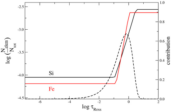
Figure 4.
Stratification of silicon and iron in the atmosphere of the star BD + 00° 1659 − twin of MX TrA. The dashed line indicates the wavelength-averaged function of the contribution of various layers to radiation in the visible range.
Two atmospheric models and corresponding synthetic SEDs were used to evaluate the effect: a chemically homogeneous model calculated for the mean abundances dex, dex, dex and a stratified one calculated taking into account the abundance gradients of Si and Fe are shown in Figure 4. The inhomogeneous horizontal distribution of elements was ignored at this step and these models were adopted for the entire atmosphere. This is justified by the fact that the current stratification analysis is not spatially resolved but is based on the radiation integrated over the visible hemisphere of the star. The difference in radiation fluxes between vertically stratified () and chemically homogeneous () models is and its wavelength dependence is shown in Figure 5 which refers to the disk-integrated flux with the homogeneous horizontal distribution of chemical elements. One can see that the maximum amplitude in the visible region reaches longward of the Balmer jump and the sign of the effect abruptly changes below Å. In the TESS bandpass, the flux difference reaches , i.e., in this case, stratification enhances the light amplitude. However, this is an upper limit. In reality, stratified spots occupy a small fraction of the surface. We need to multiply the flux of the stratified model on the filling factor corresponding to the fractional area of Si spots. Consequently, the flux ratio will be reduced by an order of magnitude. Also, the effect of stratification on emergent flux is very sensitive to the depth of the stratification step in the atmosphere as follows from the comparison with the contribution function in Figure 4. Shifting into the upper atmosphere, the step appears in a region (e.g., ) where the contribution of layers to the continuum flux is small, thus reducing the difference in flux by up to two orders of magnitude. Depending on the position of the stratification step the amplitude could both increase or decrease. The sophisticated 3D analysis with simultaneous accounting for both vertical and horizontal abundance gradients requires knowledge of the stratification profile in each surface element that is unavailable for rapidly rotating Ap stars like MX TrA. Generally, we estimate the contribution of vertical stratification to the light variations of MX TrA in the visual region as negligible, which is consistent with a good representation of the observations with horizontal abundance inhomogeneities only.
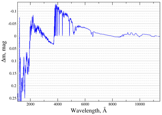
Figure 5.
Wavelength dependence of flux difference for chemically homogeneous and vertically stratified atmosphere models.
4.3. UV Variations
One of the principal effects of silicon overabundance in the atmosphere is the redistribution of flux between the far-UV and visible regions. Indeed, observations of some Ap Si stars clearly demonstrate the effect of phase shift or complete reversal of the light curve depending on the wavelength range [10,24,25]. Although photometric observations of MX TrA in the far-UV are not available, it is instructive to calculate the synthetic light curve in this region (Figure 6). We used bandpasses of two GALEX filters for far-UV (FUV, centered at Å) and near UV (NUV, at Å)3. A comparison of the two curves in Figure 6 reveals the antiphase brightness changes in NUV and FUV filters while the NUV light curve is in phase with the visual TESS one. The amplitudes are also significantly different, with the largest light variations in FUV. The physical basis for this difference is that the bandpass of the FUV filter centered shortward of 1527 Å the photoionization threshold of Si I and contains numerous resonance lines and autoionization features of Si II. Shortward ( Å) the energy is blocked due to absorption and redistributed to the longer wavelengths which leads to the flux increasing in near-UV and visual regions. This feature can be used for the photometric identification of Ap Si stars [26,27].
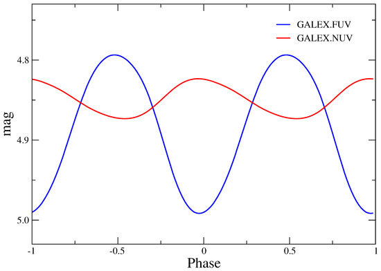
Figure 6.
Predicted ultraviolet light curves of MX TrA for FUV and NUV bands of GALEX.
Generalizing the approach, we calculated the light curves of MX TrA in the 1100–10,000 Å range with a 100 Å filter and plotted in Figure 7 the wavelength dependence of the photometric amplitude and phase of the maximum. The figure clearly illustrates the amplitude increase toward the shorter wavelengths and the existence of a dip near 2000 Å, the “null region” where the flux is almost constant over the rotational cycle. The existence of such a “null region (-s)” pointing to the mechanism of flux redistribution was previously detected in spectrophotometric observations of Ap stars [24,25,26,28]. The phases of the maximum also differ on either side of “null region”. While at the longward side, a gradual phase shift to negative values is expected at short wavelengths where the flux is effectively blocked by silicon absorption, there is a sharp increase up to a phase difference of (anti-phase variability) relative to the visual region.
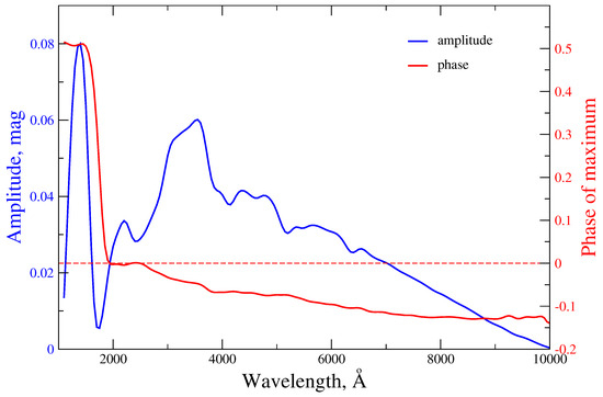
Figure 7.
Wavelength dependence of amplitude and phase of the maximum of MX TrA photometric variability caused by the inhomogeneous surface distribution of He, Si, Fe, Cr.
5. Conclusions
In the present paper, we report the results of modeling the high-precision TESS light curve of Ap Si star MX TrA based on the model of the oblique rotator and maps of surface elemental distribution previously obtained with the DI technique. We were able to successfully reproduce the observed shape of the light curve and its amplitude with an accuracy greater than 0.001 mag, accounting for the inhomogeneous surface distribution of four elements: Si, Fe, Cr, and He. This list is enough for a good fit of the observations. Diversity of the surface distributions of elements leads to a phase shift and different contributions of an individual element to the light minimum and maximum. The total synthetic light curve perfectly reproduces the shape of the observed one. The contribution of light elements: O and Mg to the light variations appears to be negligible.
We also estimated the effect of the vertical stratification of Si and Fe in the MX TrA atmosphere on the emergent flux. We show that, in principle, stratification can contribute to light variations increasing emergent flux near the Balmer jump and reducing it in the far-UV. However, in the TESS bandpass, the total effect does not exceed ∼0.01 mag and will be reduced by an order of magnitude taking into account horizontal chemical inhomogeneities. Hence, it does not contribute significantly to the TESS light curve amplitude. Empirically, we conclude that taking into account only the inhomogeneous horizontal abundance distribution of Si, Fe, Cr, and He is enough for a good representation of the observed light curve of MX TrA in the TESS bandpass.
The wavelength dependence of the amplitude of MX TrA light variations and the phase of the maximum was calculated from synthetic light curves. It shows the well-known other Ap Si star effects of increasing amplitude and antiphase variability between far-UV and visible regions. This result clearly demonstrates the possibility for the identification of new Ap Si stars, e.g., using photometric observations in the far-UV with the upcoming Spektr-UF (WSO-UV) space mission [29] and phase-correlated optical observations.
Author Contributions
Conceptualization, I.P. and T.R.; methodology, Y.P.; software, Y.P.; validation, Y.P., T.R. and I.P.; formal analysis, Y.P., I.P. and T.R.; investigation, Y.P.; resources, A.R.; data curation, A.R. and Y.P.; writing—original draft preparation, Y.P. and I.P.; writing—review and editing, Y.P., I.P. and T.R.; visualization, Y.P.; supervision, I.P.; project administration, Y.P.; funding acquisition, I.P. All authors have read and agreed to the published version of the manuscript.
Funding
This research was funded by the grant of Russian Science Foundation №24-22-00237, https://rscf.ru/en/project/24-22-00237/ (accessed on 1 August 2024).
Informed Consent Statement
Informed consent was obtained from all subjects involved in the study.
Data Availability Statement
Dataset available on request from the authors.
Acknowledgments
We obtained the observed data of the TESS space mission and processed using the SPOC (Science Processing Operations Center) automatic software package and obtained through the portal MAST (Mikulski Archive for Space Telescopes). We thank Denis Shulyak for your program LLmodels and useful tips.
Conflicts of Interest
The authors declare no conflicts of interest.
Abbreviations
The following abbreviations are used in this manuscript:
| GALEX | GALaxy evolution EXplorer-NASA orbiting space telescope |
| DI | Doppler imaging |
| LTE | Local thermodynamic equilibrium |
| NLTE | Non local thermodynamic equilibrium |
| SED | Spectral energy distribution |
| TESS | Transiting Exoplanet Survey Satellite |
| UV | Ultraviolet |
Notes
| 1 | https://mast.stsci.edu/portal/Mashup/Clients/Mast/Portal.html (accessed on 1 August 2024). |
| 2 | https://tess.mit.edu/public/tesstransients/pages/readme.html#flux-calibration (accessed on 1 August 2024). |
| 3 | https://asd.gsfc.nasa.gov/archive/galex/tools/Resolution_Response/index.html (accessed on 1 August 2024). |
References
- Michaud, G. Diffusion Processes in Peculiar a Stars. Astrophys. J. 1970, 160, 641. [Google Scholar] [CrossRef]
- Stibbs, D.W.N. A study of the spectrum and magnetic variable star HD 125248. Mon. Not. R. Astron. Soc. 1950, 110, 395. [Google Scholar] [CrossRef]
- Shulyak, D.; Tsymbal, V.; Ryabchikova, T.; Stütz, C.; Weiss, W.W. Line-by-line opacity stellar model atmospheres. Astron. Astrophys. 2004, 428, 993–1000. [Google Scholar] [CrossRef]
- Piskunov, N.E.; Rice, J.B. Techniques for Surface Imaging of Stars. Publ. Astron. Soc. Pac. 1993, 105, 1415. [Google Scholar] [CrossRef]
- Kochukhov, O. Doppler and Zeeman Doppler Imaging of Stars; Lecture Notes in Physics; Rozelot, J.P., Neiner, C., Eds.; Springer: Berlin/Heidelberg, Germany, 2016; Volume 914, p. 177. [Google Scholar] [CrossRef]
- Khan, S.A.; Shulyak, D.V. Theoretical analysis of the atmospheres of CP stars. Effects of the individual abundance patterns. Astron. Astrophys. 2007, 469, 1083–1100. [Google Scholar] [CrossRef]
- Artru, M.C.; Lanz, T. Silicon absorption in UV spectra of AP SI stars. Astron. Astrophys. 1987, 182, 273–284. [Google Scholar]
- Krtička, J.; Mikulášek, Z.; Zverko, J.; Žižńovský, J. The light variability of the helium strong star HD 37776 as a result of its inhomogeneous elemental surface distribution. Astron. Astrophys. 2007, 470, 1089–1098. [Google Scholar] [CrossRef]
- Krtička, J.; Mikulášek, Z.; Henry, G.W.; Zverko, J.; Žižovský, J.; Skalický, J.; Zvěřina, P. The nature of the light variability of the silicon star HR 7224. Astron. Astrophys. 2009, 499, 567–577. [Google Scholar] [CrossRef]
- Shulyak, D.; Krtička, J.; Mikulášek, Z.; Kochukhov, O.; Lüftinger, T. modeling the light variability of the Ap star ϵ Ursae Majoris. Astron. Astrophys. 2010, 524, A66. [Google Scholar] [CrossRef]
- Krtička, J.; Mikulášek, Z.; Lüftinger, T.; Shulyak, D.; Zverko, J.; Žižňovský, J.; Sokolov, N.A. modeling of the ultraviolet and visual SED variability in the hot magnetic Ap star CU Virginis. Astron. Astrophys. 2012, 537, A14. [Google Scholar] [CrossRef]
- Borucki, W.J.; Koch, D.; Basri, G.; Batalha, N.; Brown, T.; Caldwell, D.; Caldwell, J.; Christensen-Dalsgaard, J.; Cochran, W.D.; DeVore, E.; et al. Kepler Planet-Detection Mission: Introduction and First Results. Science 2010, 327, 977. [Google Scholar] [CrossRef]
- Weiss, W.W.; Rucinski, S.M.; Moffat, A.F.J.; Schwarzenberg-Czerny, A.; Koudelka, O.F.; Grant, C.C.; Zee, R.E.; Kuschnig, R.; Mochnacki, S.; Matthews, J.M.; et al. BRITE-Constellation: Nanosatellites for Precision Photometry of Bright Stars. Publ. Astron. Soc. Pac. 2014, 126, 573. [Google Scholar] [CrossRef]
- Ricker, G.R.; Winn, J.N.; Vanderspek, R.; Latham, D.W.; Bakos, G.Á.; Bean, J.L.; Berta-Thompson, Z.K.; Brown, T.M.; Buchhave, L.; Butler, N.R.; et al. Transiting Exoplanet Survey Satellite (TESS). J. Astron. Telesc. Instruments Syst. 2015, 1, 014003. [Google Scholar] [CrossRef]
- Paunzen, E.; Maitzen, H.M. New variable chemically peculiar stars identified in the HIPPARCOS archive. Astron. Astrophys. Suppl. Ser. 1998, 133, 1–6. [Google Scholar] [CrossRef]
- Potravnov, I.; Ryabchikova, T.; Piskunov, N.; Pakhomov, Y.; Kniazev, A. Doppler imaging of a southern ApSi star HD 152564. Mon. Not. R. Astron. Soc. 2024, 527, 10376–10387. [Google Scholar] [CrossRef]
- Potravnov, I.; Ryabchikova, T. On the surface distribution of chromium in Ap star HD 152564. INASAN Sci. Rep. 2024, 9, 1–5. [Google Scholar]
- Jenkins, J.M.; Twicken, J.D.; McCauliff, S.; Campbell, J.; Sanderfer, D.; Lung, D.; Mansouri-Samani, M.; Girouard, F.; Tenenbaum, P.; Klaus, T.; et al. The TESS science processing operations center. In Proceedings of the Software and Cyberinfrastructure for Astronomy IV, Edinburgh, UK, 26–30 June 2016; Society of Photo-Optical Instrumentation Engineers (SPIE) Conference Series. Volume 9913, p. 99133E. [Google Scholar] [CrossRef]
- Levenberg, K. A method for the solution of certain non-linear problems in least squares. Q. Appl. Math. 1944, 2, 164–168. [Google Scholar] [CrossRef]
- Marquardt, D.W. An Algorithm for Least-Squares Estimation of Nonlinear Parameters. J. Soc. Ind. Appl. Math. 1963, 11, 431–441. [Google Scholar] [CrossRef]
- Vallenari, A.; Brown, A.G.A.; Prusti, T.; de Bruijne, J.H.J.; Arenou, F.; Babusiaux, C.; Biermann, M.; Creevey, O.L.; Ducourant, C.; Evans, D.W.; et al. Gaia Data Release 3. Summary of the content and survey properties. Astron. Astrophys. 2023, 674, A1. [Google Scholar] [CrossRef]
- Bailey, J.D.; Landstreet, J.D. Abundances determined using Si ii and Si iii in B-type stars: Evidence for stratification. Astron. Astrophys. 2013, 551, A30. [Google Scholar] [CrossRef]
- Romanovskaya, T.; Potravnov, I.; Piskunov, N. Abundance and stratification analysis of slowly-rotating Si-star BD+00°1659 as a benchmark for ApSi-stars studies. Galaxies, 2024; in preparation. [Google Scholar]
- Sokolov, N.A. Ultraviolet variability of the magnetic chemically peculiar star 56 Arietis. Mon. Not. R. Astron. Soc. 2006, 373, 666–676. [Google Scholar] [CrossRef][Green Version]
- Sokolov, N.A. Ultraviolet variability of the helium-peculiar star a Centauri. Mon. Not. R. Astron. Soc. 2012, 426, 2819–2831. [Google Scholar] [CrossRef][Green Version]
- Jamar, C. Ultraviolet variations of the Ap Si stars. Astron. Astrophys. 1978, 70, 379–388. [Google Scholar]
- Romanovskaya, A.M.; Shulyak, D.V.; Ryabchikova, T.A.; Sitnova, T.M. Fundamental parameters of the Ap-stars GO and, 84 UMa, and κ Psc. Astron. Astrophys. 2021, 655, A106. [Google Scholar] [CrossRef]
- Molnar, M.R. Ultraviolet photometry form the Orbiting Astronomical Observatory. VII. alpha2 Canum Venaticorum. Astrophys. J. 1973, 179, 527. [Google Scholar] [CrossRef]
- Shustov, B.M.; Sachkov, M.E.; Sichevsky, S.G.; Arkhangelsky, R.N.; Beitia-Antero, L.; Bisikalo, D.V.; Bogachev, S.A.; Buslaeva, A.I.; Vallejo, J.C.; Gomez de Castro, A.I.; et al. WSO-UV Project: New Touches. Sol. Syst. Res. 2021, 55, 677–687. [Google Scholar] [CrossRef]


Disclaimer/Publisher’s Note: The statements, opinions and data contained in all publications are solely those of the individual author(s) and contributor(s) and not of MDPI and/or the editor(s). MDPI and/or the editor(s) disclaim responsibility for any injury to people or property resulting from any ideas, methods, instructions or products referred to in the content. |
© 2024 by the authors. Licensee MDPI, Basel, Switzerland. This article is an open access article distributed under the terms and conditions of the Creative Commons Attribution (CC BY) license (https://creativecommons.org/licenses/by/4.0/).