Abstract
M dwarfs are main sequence stars and they exist in all stages of galaxy evolution. As the living fossils of cosmic evolution, the study of M dwarfs is of great significance to the understanding of stars and the stellar populations of the Milky Way. Previously, M dwarf research was limited due to insufficient spectroscopic spectra. Recently, the data volume of M dwarfs was greatly increased with the launch of large sky survey telescopes such as Sloan Digital Sky Survey and Large Sky Area Multi-Object Fiber Spectroscopy Telescope. However, the spectra of M dwarfs mainly concentrate in the subtypes of M0–M4, and the number of M5–M9 is still relatively limited. With the continuous development of machine learning, the generative model was improved and provides methods to solve the shortage of specified training samples. In this paper, the Adversarial AutoEncoder is proposed and implemented to solve this problem. Adversarial AutoEncoder is a probabilistic AutoEncoder that uses the Generative Adversarial Nets to generate data by matching the posterior of the hidden code vector of the original data extracted by the AutoEncoder with a prior distribution. Matching the posterior to the prior ensures each part of prior space generated results in meaningful data. To verify the quality of the generated spectra data, we performed qualitative and quantitative verification. The experimental results indicate the generation spectra data enhance the measured spectra data and have scientific applicability.
1. Introduction
The traditional method to address spectral classification of stars is to combine their photometric and spectroscopic data together. The most commonly used Harvard stellar spectral classification system was proposed by the Harvard University Observatory in the late 19th century [1]. In accordance with the order of the surface temperature of the star, the system divides the stellar spectra into O, B, A, F, G, K, M, and other types [2].
M dwarfs are the most common stars in the Galaxy [3] and are characterized by low brightness, small diameter and mass, and a surface temperature around or lower than 3500 K. With the nuclear fusion speed inside the M dwarfs being slow, M dwarfs tend to have a long life span, and they exist in all stages of the evolution of the Galaxy [4]. A huge number of spectra are obtained with the emergence of sky survey telescopes, such as Sloan Digital Sky Survey (SDSS) [5,6] and Large Sky Area Multi-Object Fiber Spectroscopy Telescope (LAMOST) [7,8].
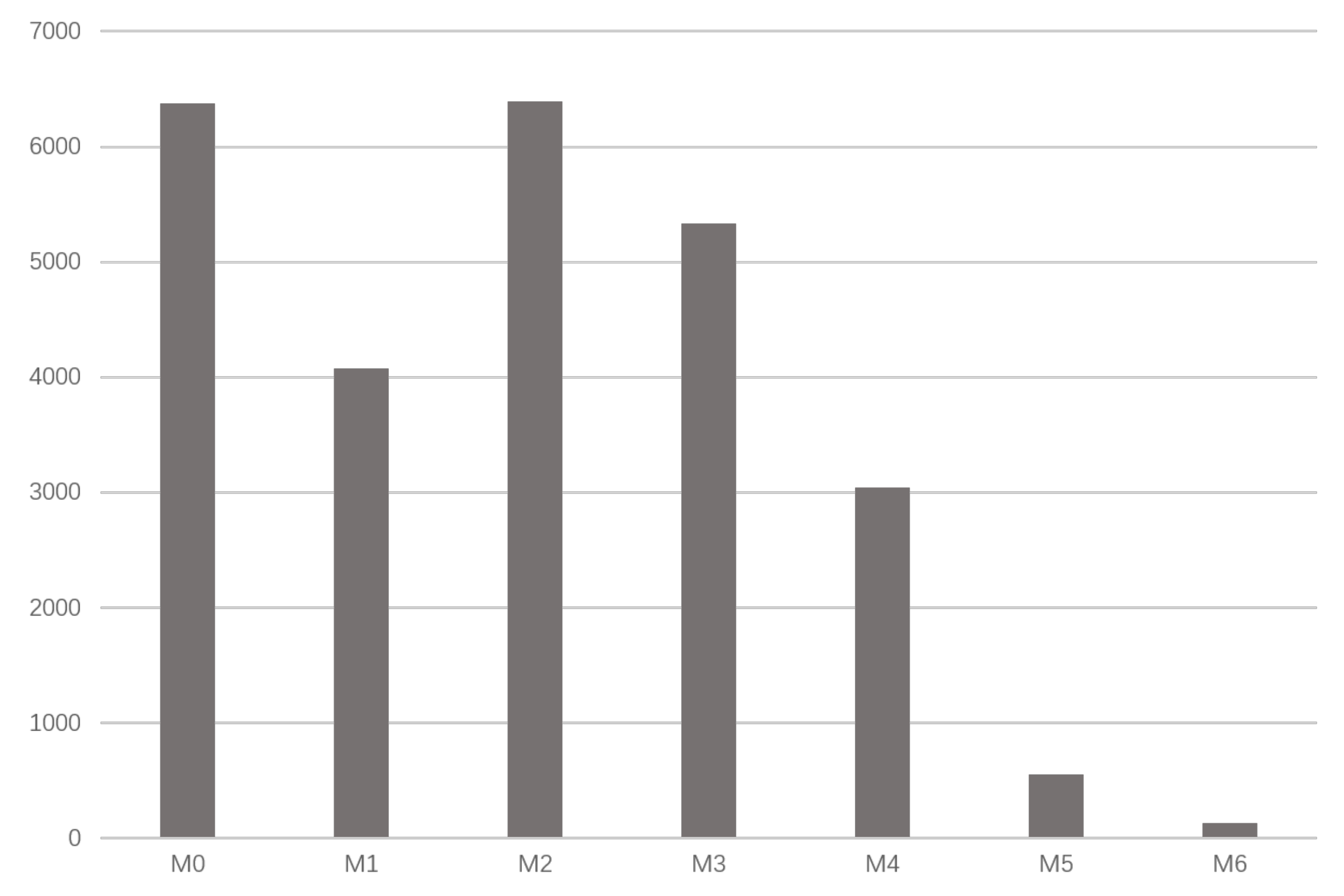
However, the distribution of the subtypes is unbalanced. In the SDSS-DR15, as shown in Figure 1, the spectra of M0–M4 are relatively greater in number, whereas that of M5–M9 is limited. The generation of specific subtype spectra of M dwarfs is helpful to solve the problem of unbalanced distribution and provide more reliable samples for research. For example, in the SDSS dataset, the number of M5–M9 is very low. When the data are limited, it is difficult for astronomers to analyze them using machine learning or deep learning methods, such as classification, clustering, dimensionality reduction, etc. If we can effectively expand the data, we can improve the M Dwarf dataset to better understand these stars. In this study, we select M-class stars with unbalanced distribution of subtypes M0–M6 (signal-to-noise ratio > 5) to verify the effectiveness of our method.

Figure 1.
Distribution of M0–M6 dwarfs with signal-to-noise ratio > 5 of Sloan Digital Sky Survey (SDSS) 15.
With the development of machine learning and deep learning, generation models were remarkably improved. An increasing number of methods are proposed to solve the lack of data, and all kinds of data, especially the two-dimensional data from the real world, were expanded effectively. AutoEncoder is a kind of neural network. After encoding and decoding, it can obtain output similar to the input. The Variational AutoEncoder (VAE), a model proposed by Kingma and Welling [9], combines variational Bayesians with neural network and achieves good results with data generation. Generative Adversarial Nets (GAN) is a model proposed by Goodfellow et al. [10] to solve the lack of data, especially for the 2D data from the real world [10,11,12,13,14]. GAN consists of a discriminator and a generator. The discriminator is designed to determine whether the input data are real or fake data generated by the generator, and the task of the generator is to generate fake data that can confuse the discriminator as much as possible. Through such a dynamic game process, similar data are generated.
The Adversarial AutoEncoder (AAE) is a model proposed by Makhzani et al. [15]. The AAE replaces the generator of the traditional generation model, GAN, with an AutoEncoder that can better learn the feature of discrete data. At the same time, the discriminator is used to correct the distribution after encoding. By doing this, the problem of traditional GAN with the generation of discrete data is solved effectively. However, due to the restriction of traditional GAN structure, the AAE also has problems, such as unstable training and model collapse, and training a good AAE with a small amount of data is difficult.
For the quality of the generated spectrum, it is necessary to qualitatively test its similarity with the original spectrum. Principal Component Analysis (PCA) [16] is a widely used data dimensionality reduction algorithm that can extract features of high-dimensional data. T-Distributed Stochastic Neighbor Embedding (t-SNE) is a visualization method for high-dimensional data proposed by by Arjovsky et al. [17]. These two methods can visually demonstrate the similarity between the observational spectra and the generated spectra.
Simultaneously, we use the generated spectrum to enhance the data of the classifier to further quantitatively verify the value of the generated spectrum. Fully connected neural network is a commonly used feature extraction method; through multilayer full connection, the feature of the spectrum can be effectively extracted. Training the classifier through two methods can visually show the performance improvement of the classifier after data expansion using the generated spectrum. The contribution of this paper could be summarized as three-fold:
- We used AAE to generate spectral data, and the model performed well with various kinds of spectral data, providing new ideas for the generation of spectral data.
- From a qualitative and quantitative perspective, we proved the high quality of the generated spectra and the effectiveness and robustness of the AAE.
- Our work provides a new direction for the combination of astronomy and machine learning.
2. Method
In this work, we propose to use an Adversarial AutoEncoder (AAE) to generate spectral data. The model is composed of a generator and a discriminator; the generator is an AutoEncoder composed of an encoder and a decoder, and the discriminator is implemented by a GAN discriminant network. AAE does not directly train the network to generate spectral data. Instead, the output of the encoder in the AutoEncoder is constrained to conform to a preselected prior distribution by the game process between the discriminator and the generator. The network parameters of autoencoder are continuously optimized to make the output of the decoder as consistent as possible with the input of the AutoEncoder. Finally, a decoder is obtained as the generator of spectral data, which can stably decode the vector that conforms to a prior distribution into high-quality spectral data.
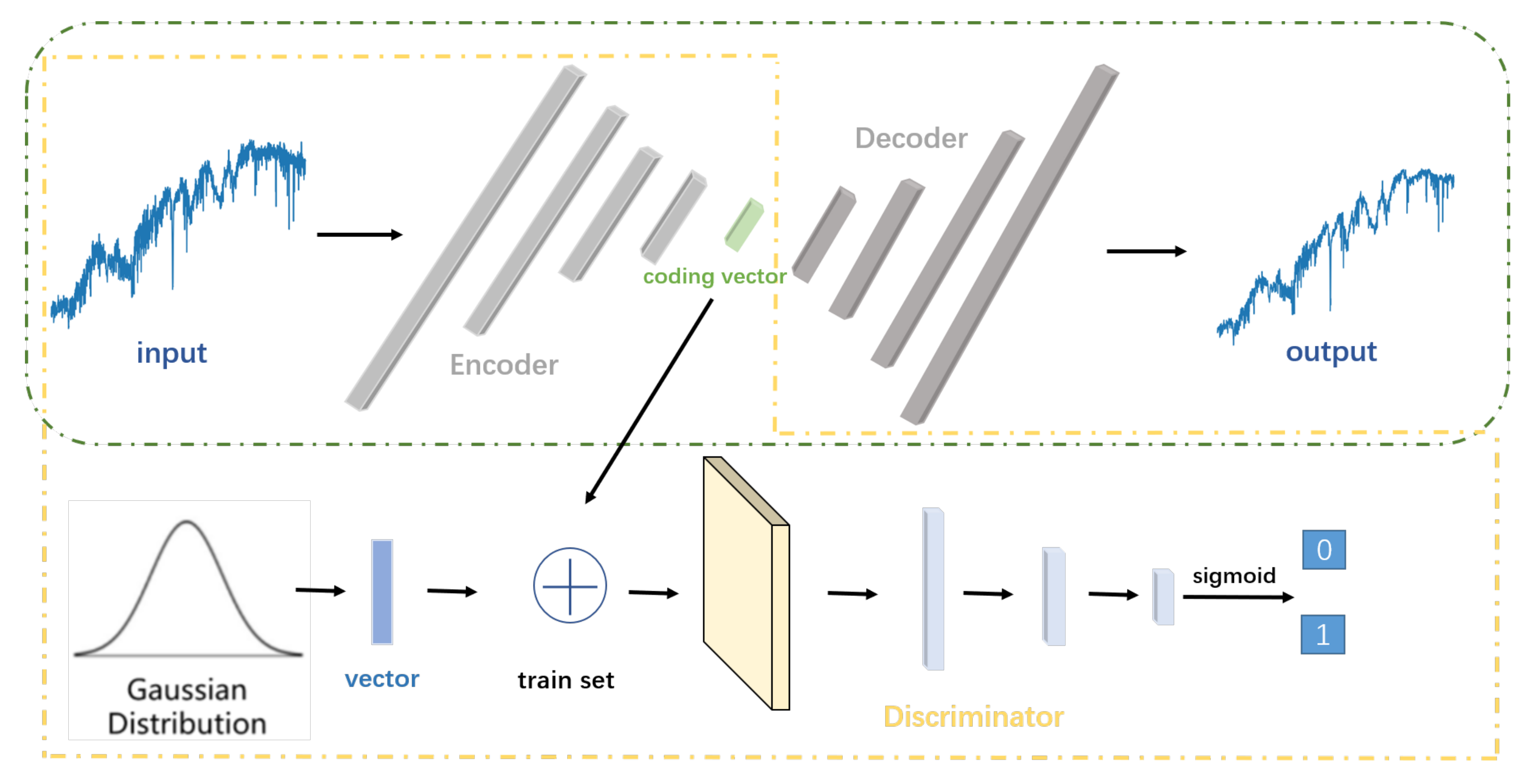
In this study, we use two fully connected neural networks to form the encoder and decoder of the AutoEncoder, and the GAN discriminant network is constituted of a two-layer, fully connected neural network. The model is shown in Figure 2. The training process is divided into two stages: the reconstruction stage, which aims to obtain a decoder that can stably reconstruct the encoding vector into high-quality spectral data, and the regularization stage, which aims to constrain the encoding vector generated by the encoder to an artificially selected prior distribution through GAN’s confrontation process.
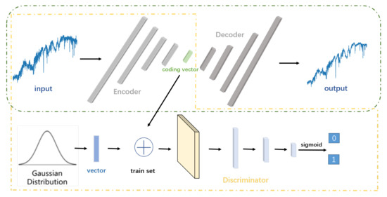
Figure 2.
Structure of the Adversarial AutoEncoder (AAE). AAE is composed of an autoencoder and a discriminator. Green box part is autoencoder composed of an encoder and a decoder, and yellow box part is a GAN composed of a discriminator and an autoencoder. Firstly, spectral data are encoded and then decoded to generate reconstructed data similar to the input data. Secondly, encoding vector of input spectral data and a randomly selected vector which conforms to the normal distribution are used as false data and real data as input of the discriminator, respectively.
Formally, we denote the encoder as Q, P as the decoder and D as the generator of the GAN. The input of the spectral data and the output of decoder are denoted as x and . The encoding vectors generated by encoder are denoted as z and are constrained to a prior distribution ; in this paper, adopts standard normal distribution. The parameter of our model is shown in Table 1:

Table 1.
Parameters of AAE.
2.1. Reconstruction Stage
In the reconstruction stage, the encoder encodes the discrete spectral data x with 3522 dimensional features into a 32-dimensional code vector z, and then restores it to a 3522-dimensional reconstruction output through a symmetrical decoder. To ensure the data reconstructed by the decoder are similar to the real data, the generated spectrum and the original spectrum use binary cross entropy as the loss function to measure the similarity between original and reconstructed data, as shown in Equation (1), and they also use the gradient descent algorithm to minimize the loss and back-propagation to update the parameters.
2.2. Regularization Stage
In the regularization stage, we conduct confrontation training similar to GAN, where the decoder of the AutoEncoder is used as the generator and the GAN discriminant network is used as the discriminator.
First, a standard normal distribution code vector with a size of 32 is randomly generated as the positive sample, and the code vector generated by the encoder is used as the negative sample. Then, the discriminator extracts the features of the input encoding vector and uses the Sigmoid activation function in the last layer of the discriminator to normalize the final output within the range of [0, 1]. The output of the discriminator represents the probability of the input being true, which determines whether the input’s distribution is closer to the real spectral data coding or the standard normal vector distribution. Therefore, the parameter optimization of the discriminator is carried out according to the idea of zero-sum game, as shown in Equation (2), which represents the probability that the discriminator successfully recognizes the real data as true and the generated data as fake.
When training the generator, we improve the generator’s ability to confuse the discriminator by optimizing the parameters of the encoder so as to minimize the probability of the discriminator successfully discriminating the generated data. As such, the encoding vector z generated by the encoder conforms to the prior distribution as much as possible, as shown in Equation (3), which represents the probability that the generated data are recognized as fake by the discriminator.
In the process of model training, the ability of decoder to reconstruct the code vector z into spectrum continuously improves, and the code vector distribution obtained by the encoder gradually approaches the standard normal distribution simultaneously. Through this model, we obtain a decoder as the spectrum generator, which can reconstruct any vector conforming to the standard normal distribution into a high-quality target spectrum. When generating the spectrum, we first randomly generate a set of vector groups conforming to the standard normal distribution as the encoding vector, and then directly use the trained decoder as the generator to generate the spectrum. The detailed optimization procedures are summarized in Algorithm 1.
| Algorithm 1 Adversarial AutoEncoder Training Strategy. |
| Input: Target spectral data ; |
| Output: Spectrum generated by AAE; |
| 1: for do |
| 2: for each mini-batch do |
| Reconstruction phase: |
| 3: Encoding to by Q; |
| 4: Decoding to by P; |
| 5: compute Reconstruction loss between and as Equation (1) and update the |
| encoder and decode; |
| Regularization phase: |
| 6: Randomly choose vectors from a Gaussian distribution as true data |
| 7: Generate vectors from as false data by Generator G (same as Encoder P) |
| 8: Combine and as training data Z; |
| 9: Discriminating Z and compute Regularization loss as Equations (2) and (3), then |
| update Discriminator D and Generator G; |
| 10: end for |
| 11: end for |
| Generate data: |
| 12: Randomly choose vectors from a Gaussian distribution |
| 13: Use Encoder Q as Generator transforms to as generate data |
| 14: return |
2.3. Visualization of Dimensionality Reduction
PCA and t-SNE convert high-dimensional data to low-dimensional data under the premise of small information loss, which is conducive to visualization. The goal of t-SNE is to map the data distribution of the high-dimensional space into the low-dimensional space and take the difference of the probability distribution of the data in the high-dimensional and low-dimensional space as a constraint condition. We define the KL divergence to represent the difference between the two distributions; the smaller the KL divergence is, the smaller the difference is:
where and represent two different spectral data, and correspond to and in low-dimensional space, represents the variance of the Gaussian distribution constructed with as the center, represents the probability that is the neighborhood of , and represents the conditional probability that is the domain of . The gradient descent method is used to solve the optimization problem and find the minimum value of KL divergence. During iterative optimization, the data distribution in the low-dimensional space continuously gets closer to the data distribution in the high-dimensional space. Finally, the resulting low-dimensional space data can be considered the mapping of high-dimensional data in low dimensions.
3. Experiment
3.1. Spectra Acquisition and Preprocessing
A total of 25,892 M-type dwarf spectra from SDSS DR15 were obtained through Casjob 1. The subtype ranges from M0 to M6. The total number of M6 spectra we choose to generate is 127, accounting for 0.49% of the total, as shown in Table 2.
Table 2.
Number of the experimental spectra.
Then, we normalize the spectra using the following steps:
- Discard all the spectral data with a signal-to-noise ratio < 5.
- The uniform wavelength range is 3800–9000 Å, and the sampling points for each sample data is 3522.
- Normalize each sampling point of the sample data, as shown in Equation (7). The range is [0, 1].
After normalization of each spectrum, the spectra is used as the input to the AutoEncoder network.
3.2. Spectra Generation
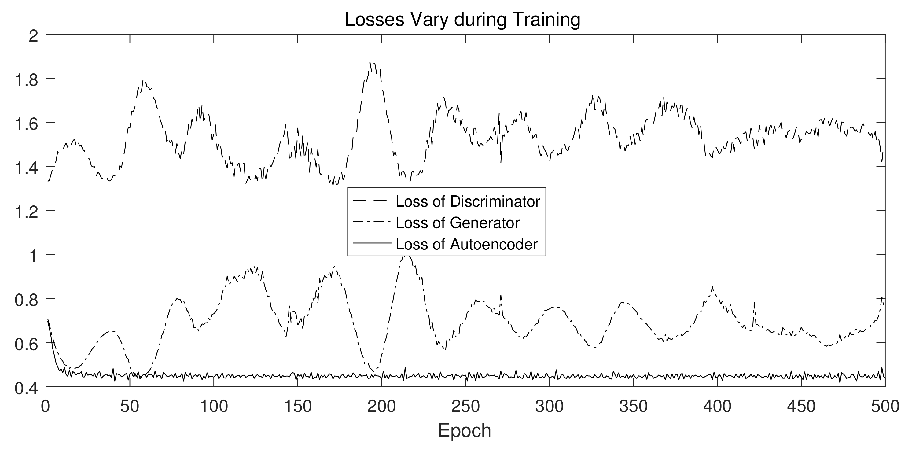
The spectra generation uses AAE to accept the original spectra as input. In 500 iterations of training, as shown in Figure 3, the loss of the autoencoder first experienced a rapid decrease and then became stable, indicating that the autoencoder part of AAE can successfully output reconstructed data that are similar to that of the input. In addition, although there are some fluctuations in the loss of the generator and the discriminator, it is basically in a state of balance, indicating that the discriminator and the generator reach equilibrium during the game process, and problems such as gradient disappearance did not occur.

Figure 3.
Loss of generator, discriminator, and autoencoder during training: – – represents loss of discriminator fluctuates in range of [1.2, 2.0], – - – - represents the loss of generator fluctuates in range of [0.4, 1.0], —— represents loss of autoencoder fluctuates in range of [0.4, 0.8].
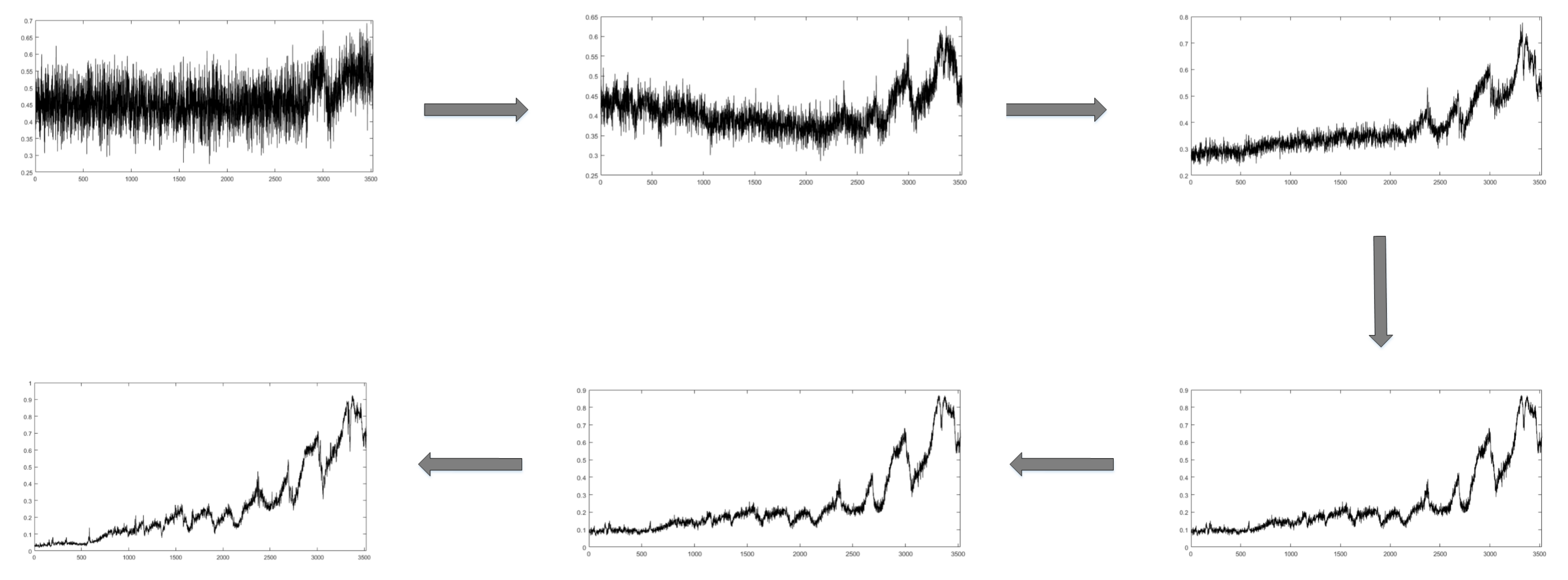
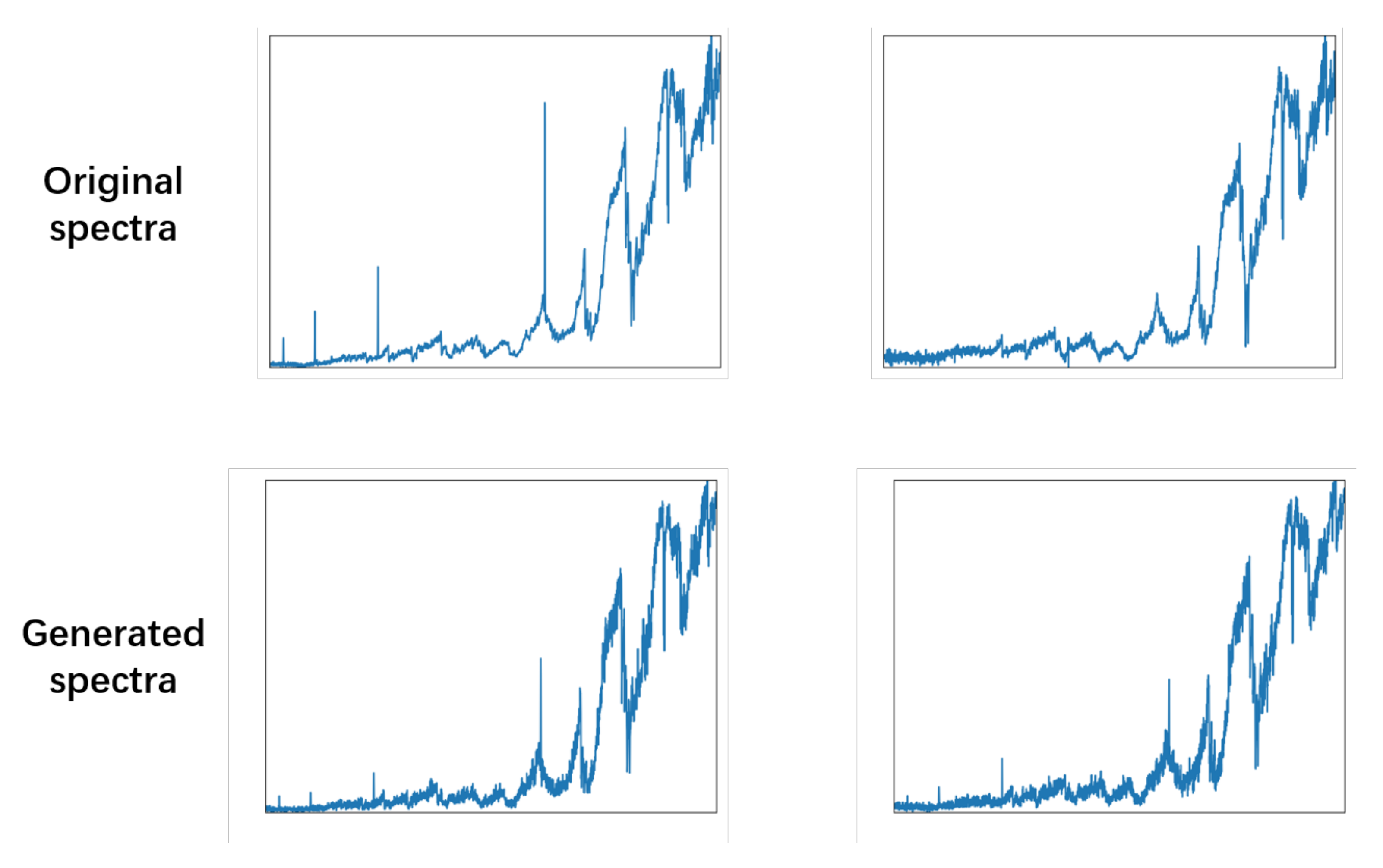
Simultaneously, the AAE gradually and steadily generates higher-quality spectral data, as shown in Figure 4 and Figure 5. With training of the model, the noise of the generated spectral data gradually decreases, the characteristic peaks are more obvious, and the signal-to-noise ratio is significantly improved. The generated spectrum and the measured spectrum are very similar in multiple characteristic peaks, and the generator learned the feature of the original spectral data.

Figure 4.
Generated spectral data during training.

Figure 5.
Compare original spectral data with generated spectral data.
3.3. Qualitative Experiment
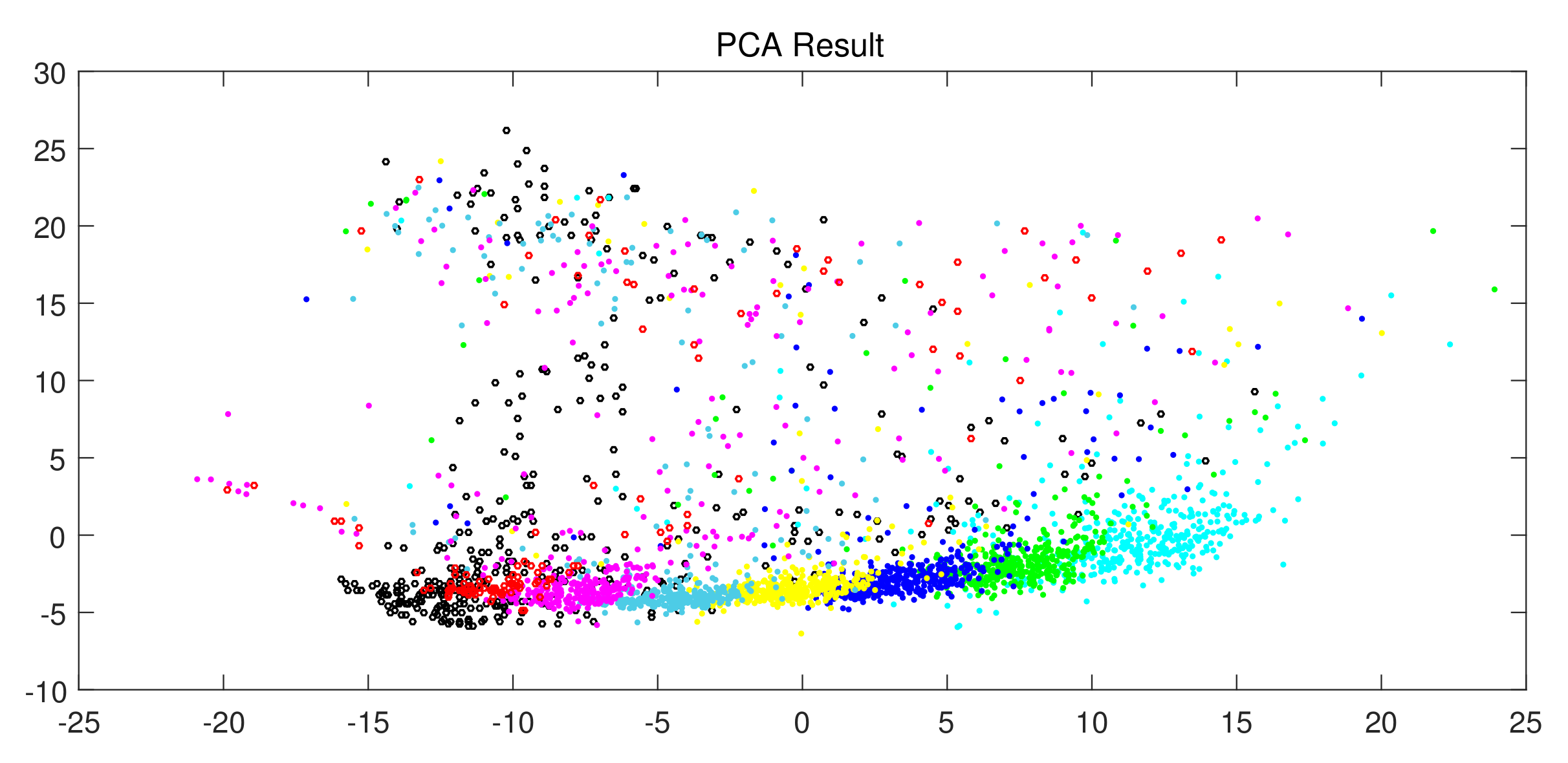
After training, a model trained against the AutoEncoder was obtained, and 400 M6 dwarf spectra (black) were generated for verification. Simultaneously, 127 measured M6 spectra (red) and 400 data of M0∼M5 dwarf were selected.
All the spectral data are reduced to two dimensions and projected by PCA, as shown in Figure 6. The black area basically surrounds the red area and is clearly distinguished from M0–M5 type dwarfs. Furthermore, a few outliers exist due to the influence of the signal-to-noise ratio.
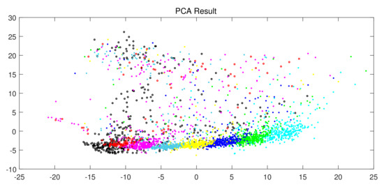
Figure 6.
Result of dimension reduction by PCA.
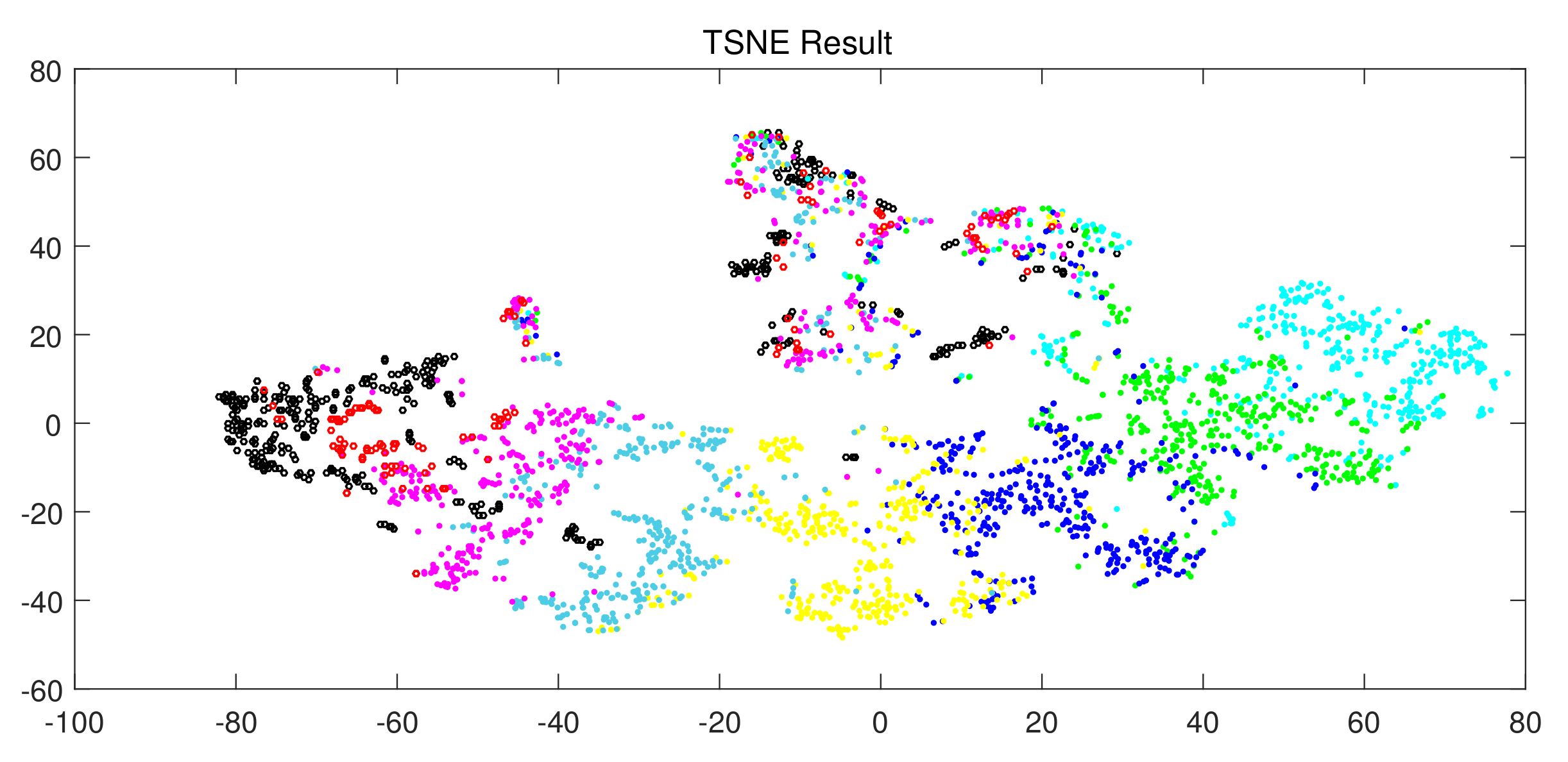
We use t-SNE to visualize the above data by dimensionality reduction, as shown in Figure 7. Most of the black areas also coincide with the red areas. Although a small part of the black area does not coincide with the red area, there are black areas near each red area, which once again proves AAE’s ability to generate the simulation data.
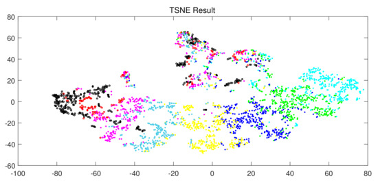
Figure 7.
Visualization result of t-SNE dimension reduction.
3.4. Quantitative Experiment
3.4.1. Evaluation Protocol
To better evaluate the results of quantitative experiments, we propose an evaluation protocol consisting of Precision (P), Recall (R), and F1-score (F). Precision quantifies the number of positive class predictions that actually belong to the positive class; Recall quantifies the number of positive class predictions made out of all positive examples in the dataset, and F1-score provides a single score that balances both the concerns of Precision and Recall in one number, as defined in (8).
True Positive () represents the number of correctly predicted positive samples; True Negative () represents the number of correctly predicted negative samples; False Positive () represents the number of incorrectly predicted positive samples; False Negative () represents the number of incorrectly predicted negative samples, as shown below in the Confusion Matrix in Figure 8.
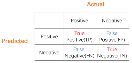
Figure 8.
Confusion Matrix.
3.4.2. Quantitative Experiment
To further quantitatively evaluate the quality of the spectrum generated by the AAE model, we used fully connected neural networks as spectral classifiers for classification, as shown in Table 3. We also chose all data from the M-type data set of M0–M6 with a signal-to-noise ratio of >5 as train data (0.75) and test data (0.25).
Table 3.
Parameters of Classifer.
Firstly, we use both the train and test data to train a classifier to verify the accuracy of generated spectral data so as to verify whether generated data could represent the desired class, as shown in Table 4. Then, we use the AAE model for data enhancement to complete all the train spectral data to 3000 to verify the enhancement of generated data for the real spectral data, as shown in Table 5.
Table 4.
Accuracy of M0–M6 data generated by AAE.
Table 5.
Classification of M0–M6 subdwarfs with data augmentation.
The quantitative experimental results of the AAE model can be analyzed. The AAE model can generate target spectral data stably and with high quality, representing the target class exactly. Data enhancement of the spectral data can not only improve the classification effect of the model, but also remit the problem of imbalanced data distribution. In the future, we will further explore the data-influencing factors on the spectral quality of the AAE generation model.
4. Discussion
In this section, we will discuss the astronomical application and the potential for further study of AAE. In case of a high cost of actual observation, AAE can generate simulation spectra to improve the M Dwarf dataset to better understand these stars in a simple way. It provides a reference method for the automatic searching of other rare and special celestial objectives in the massive spectra. This method can simulate any type of spectrum and is an innovative research method, and we will extend AAE to other types of spectra for further studies. Moreover, AAE is an extension of GAN, so it can refer to other improvements related to GAN to improve the performance of AAE in spectral data generation, such as Wasserstein GAN [18], Cycle GAN [19], and so on.
5. Conclusions
In this paper, we proposed using AAE to generate high-quality spectral data. To verify the effectiveness of AAE, we designed quantitative and qualitative experiments on M-type stars. The experimental results showed that the generated spectra can expand the original spectra, and the expanded range does not exceed one subtype, which has strong practical value and significance.
Author Contributions
Conceptualization, B.J. and J.W.; methodology, J.W.; software, J.W. and X.W.; validation, X.W. and B.L.; formal analysis, Y.C. and B.L.; investigation, X.W.; resources, B.J.; writing—original draft preparation, J.W.; writing—review and editing, J.W.; visualization, B.L. and Y.C.; supervision, B.J.; project administration, B.J.; funding acquisition, B.J. All authors have read and agreed to the published version of the manuscript.
Funding
This paper was supported by the Shandong Provincial Natural Science Foundation, China (ZR2020MA064).
Data Availability Statement
Not applicable.
Acknowledgments
This paper was supported by the Shandong Provincial Natural Science Foundation (ZR2020MA064). Funding for the Sloan Digital Sky Survey IV was provided by the Alfred P. Sloan Foundation, the U.S. Department of Energy Office of Science, and the Participating Institutions. SDSS acknowledges support and resources from the Center for High-Performance Computing at the University of Utah. The SDSS web site is www.sdss.org. We acknowledge the use of spectra from SDSS.
Conflicts of Interest
The authors declare no conflict of interest.
Note
| 1 | https://dr15.sdss.org/, accessed on 13 March 2021 |
References
- Welther, B.L. Discoveries, Achievements, and Personalities of the Women Who Evolved the Harvard Classification of Stellar Spectra: Williamina Fleming, Antonia Maury, and Annie Jump Cannon. Available online: https://ui.adsabs.harvard.edu/abs/2010AAS...21520004W/abstract (accessed on 31 August 2021).
- Gray, R.O.; Corbally, C.J. Stellar Spectral Classification; Princeton University Press: Princeton, NJ, USA, 2009. [Google Scholar]
- Fischer, D.A.; Marcy, G.W. Multiplicity among M Dwarfs. Astrophys. J. 1992, 396, 178. [Google Scholar] [CrossRef]
- Bessell, M.S. The Late M Dwarfs. Astron. J. 1991, 101, 662. [Google Scholar] [CrossRef]
- Yanny, B.; Rockosi, C.; Newberg, H.J.; Knapp, G.R.; Adelman-McCarthy, J.K.; Alcorn, B.; Allam, S.; Allende Prieto, C.; An, D.; Anderson, K.S.J.; et al. SEGUE: A Spectroscopic Survey of 240,000 Stars with g = 14–20. Astron. J. 2009, 137, 4377–4399. [Google Scholar] [CrossRef] [Green Version]
- Blanton, M.R.; Bershady, M.A.; Abolfathi, B.; Albareti, F.D.; Allende Prieto, C.; Almeida, A.; Alonso-García, J.; Anders, F.; Anderson, S.F.; Andrews, B.; et al. Sloan Digital Sky Survey IV: Mapping the Milky Way, Nearby Galaxies, and the Distant Universe. Astron. J. 2017, 154, 28. [Google Scholar] [CrossRef]
- Cui, X.Q.; Zhao, Y.H.; Chu, Y.Q.; Li, G.P.; Li, Q.; Zhang, L.P.; Su, H.J.; Yao, Z.Q.; Wang, Y.N.; Xing, X.Z.; et al. The large sky area multi-object fiber spectroscopic telescope (LAMOST). Res. Astron. Astrophys. 2012, 12, 1197. [Google Scholar] [CrossRef]
- Zhao, G.; Zhao, Y.H.; Chu, Y.Q.; Jing, Y.P.; Deng, L.C. LAMOST spectral survey — An overview. Res. Astron. Astrophys. 2012, 12, 723–734. [Google Scholar] [CrossRef] [Green Version]
- Kingma, D.P.; Welling, M. Auto-Encoding Variational Bayes. arXiv 2014, arXiv:1312.6114. [Google Scholar]
- Goodfellow, I.J.; Pouget-Abadie, J.; Mirza, M.; Xu, B.; Warde-Farley, D.; Ozair, S.; Courville, A.; Bengio, Y. Generative adversarial networks. arXiv 2014, arXiv:1406.2661. [Google Scholar]
- Radford, A.; Metz, L.; Chintala, S. Unsupervised Representation Learning with Deep Convolutional Generative Adversarial Networks. arXiv 2015, arXiv:1511.06434. [Google Scholar]
- Lucic, M.; Kurach, K.; Michalski, M.; Gelly, S.; Bousquet, O. Are gans created equal? A large-scale study. arXiv 2017, arXiv:1711.10337. [Google Scholar]
- Ledig, C.; Theis, L.; Huszar, F.; Caballero, J.; Cunningham, A.; Acosta, A.; Aitken, A.; Tejani, A.; Totz, J.; Wang, Z. Photo-Realistic Single Image Super-Resolution Using a Generative Adversarial Network. Available online: https://openaccess.thecvf.com/content_cvpr_2017/papers/Ledig_Photo-Realistic_Single_Image_CVPR_2017_paper.pdf (accessed on 31 August 2021).
- Gui, J.; Sun, Z.; Wen, Y.; Tao, D.; Ye, J. A review on generative adversarial networks: Algorithms, theory, and applications. arXiv 2020, arXiv:2001.06937. [Google Scholar]
- Makhzani, A.; Shlens, J.; Jaitly, N.; Goodfellow, I.; Frey, B. Adversarial autoencoders. arXiv 2015, arXiv:1511.05644. [Google Scholar]
- Ke, N.Y.; Sukthankar, R. PCA-SIFT: A more distinctive representation for local image descriptors. In Proceedings of the IEEE Computer Society Conference on Computer Vision & Pattern Recognition, Washington, DC, USA, 27 June–2 July 2004. [Google Scholar]
- Van der Maaten, L.; Hinton, G. Visualizing data using t-SNE. J. Mach. Learn. Res. 2008, 9, 2579–2605. [Google Scholar]
- Arjovsky, M.; Chintala, S.; Bottou, L. Wasserstein generative adversarial networks. In Proceedings of the International Conference on Machine Learning (PMLR), Sydney, Australia, 6–11 August 2017; pp. 214–223. [Google Scholar]
- Almahairi, A.; Rajeswar, S.; Sordoni, A.; Bachman, P.; Courville, A. Augmented CycleGAN: Learning Many-to-Many Mappings from Unpaired Data. In Proceedings of the International Conference on Machine Learning, Stockholm, Sweden, 10–15 July 2018. [Google Scholar]

Publisher’s Note: MDPI stays neutral with regard to jurisdictional claims in published maps and institutional affiliations. |
© 2021 by the authors. Licensee MDPI, Basel, Switzerland. This article is an open access article distributed under the terms and conditions of the Creative Commons Attribution (CC BY) license (https://creativecommons.org/licenses/by/4.0/).