Advanced Path Planning for Autonomous Street-Sweeper Fleets under Complex Operational Conditions

Abstract

In recent years, autonomous mobile platforms have seen an increase in usage in several applications. One of which is street-sweeping. Although street-sweeping is a necessary process due to health and cleanliness, fleet operations are difficult to plan optimally. Since each vehicle has several constraints (battery, debris, and water), path planning becomes increasingly difficult to perform manually. Additionally, in real-world applications vehicles may become inactive due to a breakdown, which requires real-time scheduling technology to update the paths for the remaining vehicles. In this paper, the fleet street-sweeping problem can be solved using the proposed lower-level and higher-level path generation methods. For the lower level, a Smart Selective Navigator algorithm is proposed, and a modified genetic algorithm is used for the higher-level path planning. A case study was presented for Uchi Park, South Korea, where the proposed methodology was validated. Specifically, results generated from the ideal scenario (all vehicles operating) were compared to the breakdown scenario, where little to no difference in the overall statistics was observed. Additionally, the lower-level path generation could yield solutions with over 94% area coverage.

1. Introduction

Unmanned ground vehicles (UGVs) have seen an increase in popularity amongst operations researchers in recent years. Spanning over several applications such as autonomous cleaning [1,2], lawn mowing [3], surveillance [4], tillage [5], and street-sweeping [6], UGVs can be applied seamlessly to many coverage path planning (CPP) problems. Additionally, UGVs can be used individually or in fleets. When using UGVs in fleets, the efficiency can increase, and overall operation time can decrease at the expense of complicated fleet management strategies [7,8]. In this paper, fleet management technology and global path planning for UGV street-sweeping will be the focus.

Compared to other UGV applications, street-sweeping operations are more complex because of the increased number of constraints. Specifically, street-sweepers disperse water (to make sweeping small particles easier), accumulate debris, and drain the battery via normal operation. Typically, a depot serves as the facility where the battery can be charged, the water can be refilled, and the debris can be disposed of. During operation, the status of all the respective constraints should be carefully monitored, and depot trips can be conducted as necessary. The problem becomes increasingly more complex when fleets of UGV street-sweepers are to be managed. Complications arise when street sweepers become inactive during operation due to an unexpected breakdown. In these cases, the remainder of the path allocated to the out-of-service vehicle is left untouched. Ideally, the remainder of the unvisited path for the out-of-service vehicle should be covered by the remaining vehicles in an efficient manner.

The CPP problem relates to the problem where an entity (robot, vehicle, etc.) is assigned the task of traveling over an area. The area may be large, small, complicated, simple, and have obstacles, but the task remains the same. The CPP can be formulated as a variant of the traveling salesman problem (TSP) called the covering salesman problem (CSP) [9]. In the TSP, the optimal traversal sequence for all nodes should be found, whereas the optimal traversal sequence of a subset of nodes should be found in the CSP [10]. In the CSP, the vehicle width must be considered, so an edge with a predetermined offset (modeling the vehicle width) may cover some of the required nodes without directly visiting them; hence, only a subset of nodes can be visited.

It is common to see the CPP problem be applied to large and complicated areas. In these cases, the problem can be divided into several smaller feasible areas by using cellular decomposition methods. Then, a local path planner can be used to find the coverage path in each cell (typically an exhaustive sweep of the cell), and a global path planner can be used to find the optimal traversal sequence of the cells. Several methods have been explored in the literature to perform such decomposition, such as boustrophedon cell decomposition [11], morse cell decomposition [12], and trapezoidal decomposition [13]. Each method has its own application, which is dependent on the problem requirements and environmental complexity.

Within the targeted area (or sub-area in the case of cell decomposition), the optimal path to the CPP problem should be found. In the literature, the CPP algorithms can be divided into two classes: classical and heuristic-based algorithms [14]. Several algorithms exist within the classical type algorithms, such as random walk (RW) and chaotic coverage. The chaotic coverage algorithms can be characterized by topological transitivity and sensitive dependence on initial conditions for a mobile robot [15]. Typically, to perform such chaotic movements, the controller for the mobile robot is built with a combination of chaotic dynamic variables and kinematic equations that predict the trajectory of the robot [15]. Some examples of chaotic systems include the Arnold system [15,16] and the Lorenz system [17]. For the RW, a robot moves within the target environment until a collision with an obstacle is detected. In the linear case, the robot will continuously travel linearly until a collision with an obstacle is detected. When this occurs, the next trajectory will be randomly selected within the bounds of the target area [18,19]. Additionally, a spiral motion can also be used [20]. The classical methods are typically continuous and do not guarantee total area coverage [21], so additional methods were developed to overcome these limitations.

Contrary to the classical methods, additional methods operate using a discrete model of the environment. This can be thought of as a grid-like structure where each cell has a connection to all adjacent cells, also known as a graph. In these cases, greedy search or graph search algorithms can be applied to solve the coverage path. The well-studied Dijkstra’s algorithm has been used to solve the CPP [22]. However, due to its greedy nature, the global optimal cannot be guaranteed [23]. Additional methods can be used instead, such as the depth-first search (DFS) and breadth-first search (BFS). DFS has been used for CPP in [24] for cleaning applications, and BFS has been used in [25] for aerial remote sensing. Some issues regarding DFS and BFS have been noted in the literature. Specifically, DFS fails to yield optimal paths in infinite-depth spaces, and BFS consumes large amounts of memory due to the branching technique applied [26].

Additionally, heuristic-based approaches can be used to solve the CPP. The heuristic-based approaches include two categories of algorithms: evolutionary algorithms and human-inspired algorithms. In evolutionary algorithms, a population of search agents is used to model the CPP, and over several iterations (the exploration stage), the search agents can exploit the global optimal solution. In the human-inspired techniques, models mimic the way the human brain works by learning what ideal solutions look like (reinforced learning). Upon completion of the training stage, the model can predict the optimal path for a CPP problem.

As previously stated, the CPP can be modeled as the TSP or CSP. This problem model makes implementing the genetic algorithm (GA) very easy. In the genetic algorithm, the sequence of nodes to be visited is optimized via selection, crossover, and mutation over several iterations [27]. The objective for this case is simply to find the minimum cost path that visits all the required nodes in the TSP or the minimum cost path that covers all the required nodes in the CSP. The fitness function in the GA is easy to change, thus making it very flexible for different categories of the CPP problem. The GA has been used in several studies in the CPP domain with success [3,11,28], thus making it a great starting point for the CPP problem.

With regard to dividing the workload amongst several homogeneous vehicles, some researchers have referred to this problem as the vehicle path planning and scheduling problem (VPPSP) [29]. By using an effective scheduling strategy, the overall operation time can be greatly reduced with a fleet of vehicles in comparison to one [30]. In the VPPSP, a set of autonomous vehicles should visit a set of targets, and each vehicle’s path should begin and end at the depot. In [29], a modified version of the GA was proposed to solve the VPPSP. In a separate study, the CPP for a fleet of unmanned aerial vehicles (UAV) was solved using the integer programming (IP) formulation [31]. Their work provided solutions that operate within the constraints of the UAVs. Another study uses a cellular decomposition method to divide a large area into several smaller ones; then, the areas are continuously assigned to UAVs until the constraints are violated [32]. In each of the sub-areas, a zig-zag pattern is used to cover the area.

Additional studies have focused on the path planning of robotic fleets as a single unit. A large portion of these studies focus on formation control schemes where robots are instructed to maintain a desired formation while following a global path. In one study, a leader-follower control scheme was developed to solve the translational maneuvering problem for robotic fleets [33]. Their control law consists of individual tracking errors and coordination tracking errors for leader-follower pairs. Another study uses a similar approach but in more complex environments with obstacles [34]. In this study, two separate control algorithms based on the model predictive control (MCP) scheme were proposed, namely the linear and non-linear MPC. Their methods show improvements over other methods for maintaining formation while simultaneously avoiding static obstacles. Another study focuses on the control scheme for dynamic formations [35]. In this study, the formation-control problem was modeled as a synchronization control problem specific to the formation requirements. Then, a synchronous controller was used by each robot to ensure that the position and errors were minimized. Simulations and experimental studies validate the effectiveness of the proposed approach. In the mentioned studies, a common goal for the robot fleet is to achieve the desired formation such that the fleet moves as a single unit. However, these studies do not focus on separating the fleet to achieve a goal. Additionally, there is a large focus on the path tracking, and the path planning has not been discussed.

Some studies have considered the failure of mobile robots in fleets. Due to the difference in the expected workload in the event of a vehicle failure, the planned routes will need to be modified to ensure a proper workload balance [36]. When a vehicle failure occurs, several different approaches may be used to redistribute the remaining paths of the out-of-service robot to the remaining ones. In one paper, a simple approach is proposed called the First-Responder (FR). In the FR, any robot that finishes its route can cover the remaining routes from broken vehicles [37]. Since this approach does not use any optimization techniques, it was improved by the authors in a later study. In this study, the authors propose an optimization technique to redistribute the paths amongst the remaining robots called Cooperative Autonomy for Resilience and Efficiency (CARE) [38]. In CARE, the authors were able to improve their FR approach by using a distributed discrete event supervisor to trigger games amongst the remaining robots in the fleet. The games consist of the no-idling game and the resilience game, which are triggered when a robot completes its route and when a robot fails, respectively. The CARE approach shows complete coverage under failures and reduced coverage time.

In the mentioned literature, existing studies discuss area partitioning using decomposition methods, local path planning methods within the sub-areas, and techniques to manage fleet operations for the CPP. From the mentioned literature, not all these techniques have been applied to the autonomous street-sweeping fleet CPP problem. Additionally, a portion of fleet robotic research aims to maintain the formation of a fleet of mobile robots while following a planned path. This research fails to separate the fleet to achieve a goal and instead focuses on moving the fleet as a whole while following a path. This may be beneficial for applications such as highway street-sweeping, where a fleet can cover several lanes simultaneously with a relatively consistent path defined by the road. These approaches work under the assumption that an optimal path has already been planned, and the fleet is now being instructed to follow it using tracking control strategies. However, there is a lack of research involved in the optimization of the planned path for robotic fleets, which is the focus of this study. It means that the research presented in this study aims to separate the fleet and generate the optimal path for each individual vehicle. Additionally, robotic formations cause problems in complex areas such as walking paths since the formation cannot fit within the bounds of the targeted areas, thus requiring individual paths for each vehicle.

Few studies have examined the breakdown scenario in which a vehicle becomes unavailable during operation for a fleet of autonomous street-sweepers. In the above literature, breakdown scenarios have been considered, but the complex constraints of street sweeping require additional consideration. For example, it may be better for a vehicle with more room in the debris hopper to service the remaining route of one vehicle. Or it may be better for a vehicle nearing the debris capacity to cover the remaining paths near the depot so a short distance can be traveled to dispose of the debris. Such complex constraints have not been considered in the existing literature and require additional methods for proper implementation and consideration. So, the following research aims to fill this gap by applying a lower-level path generation method to calculate the coverage path in each sub-area and a higher-level path generation method to divide the sub-areas amongst the autonomous street-sweepers while selecting the optimal start location for each sub-area. The proposed route optimization techniques can consider several real-world constraints that are specific to street-sweeping (debris, water, battery, and vehicle breakdown conditions) while also providing near-optimal results for the NP-hard problem. Additionally, the proposed methods can be applied in breakdown scenarios to redistribute the un-serviced path (from the broken vehicle) to the remaining vehicles. A case study for Uchi Park Zoo will be presented to show the effectiveness of the developed algorithm.

The remainder of the article is organized as follows: Section 2 discusses the methods used to solve the lower and higher-level path planning problems, Section 3 discusses the problem-specific parameters for the case study in Uchi Park Zoo and the graph generation methods for the lower and higher-level optimization, Section 4 presents results for two operational conditions (two normal vehicles, and one normal vehicle with a vehicle that breaks down) in Uchi Park Zoo, and Section 5 concludes the following research.

2. Route Generation Methodology

Previous research has discussed several approaches for solving the CPP. However, existing methods have not considered complex operational constraints related to autonomous street-sweeping when generating routes, which makes them difficult to apply to this specific set of CPPs. Additionally, previous methods have explored the occurrence of failures in fleet robotic operations but similarly lack the ability to handle the complex constraints of autonomous street-sweeping.

Lower-level and higher-level path planning algorithms were developed to overcome such limitations. The lower-level path generation creates the optimal coverage path within each sub-area, while the higher-level path generation creates the total path for each vehicle while considering the respective constraints. The lower-level path generation is composed of a novel route optimization algorithm named the Smart Selective Navigator (SSN), and the higher-level path generation makes use of a modified version of the GA. Higher-level path generation is also responsible for generating complete routes that include depot trips as necessary (when the water or debris capacity is met). Both path-generation methods will be explained in detail in this section.

For the proposed methods to work, it is assumed that a target area has been converted into a graph structure and that the total graph is divided into several sub-areas that are to be serviced. Each sub-area may have serviceable and non-serviceable edges. The sub-area division can be performed automatically (as seen in literature as the decomposition method) or manually for logistical purposes, and each sub-area can have several candidates starting locations with predetermined endpoints.

2.1. Lower-Level Path Generation

A novel algorithm named the Smart Selective Navigator (SSN) was used to generate the lower-level paths. However, any other route optimization methods can be used in this stage. The purpose of the lower-path generation is to pre-process several candidate paths for each sub-area such that the optimal one is selected by the higher-level path generation algorithm (which will be discussed in the next section). The SNN is a non-backtracking heuristic method created for logistics problems. SSN is a turn-based approach that assigns jobs (serviceable edges) to idle vehicles at each Time Interval (TI). This method can handle multiple vehicles at the same time and incorporate many different constraints such as fuel restriction, turn restriction, etc. Instead, the vehicle constraints are handled in the higher-level path generation (which will be discussed in the next section). However, it is assumed that only a single vehicle is used, and it is equipped with enough resources to service the entire area. In the SSN, the vehicle should have a predefined starting point, and the vehicle will continue to service the graph until one of the following conditions are met:

• All the required edges are serviced;
• The generated path length exceeds a given threshold.

The second condition is defined to prevent vehicles from getting stuck in loops. The quality of the routes created using the SSN can be calculated using Equation (1).

$$cost=\left(total operation time+time penalty\right)\times (remaining edges+1)$$

(1)

In Equation (1), the $remaining edges$ is the number of edges that were supposed to be serviced but were not due to the second stop condition. In the ideal case, the $remaining edges$ will be 0, but this is not the case for the initial solutions produced using SSN. Additionally, a $time penalty$ is applied to the paths created using SSN, which can be formulated in Equation (2). The time penalty is applied to penalize sharp turns that are difficult for vehicles to perform. In Equation (2), it is assumed that a 180° turn (u-turn) takes 10 s to perform, so any other turn is a fraction of this. This was considered because the turn radius was not directly integrated into the lower-level graphs.

$$time penalty=\frac{turning angle}{180}\times 10$$

(2)

As previously stated, SSN operates using a turn-based approach to assign jobs to the vehicle at each TI. At each TI, the vehicle’s current position is acquired ($n_i$), then the score of all neighboring nodes ($n_j$) is calculated. The edge created ($e_k=(n_i,n_j$)) by the neighboring node with the best score will be assigned to the vehicle. The score for neighboring nodes can be calculated using Equation (3) where $x_1$ − $x_5$ are coefficients that need to be optimized (using a GA), and each sub-score in Equation (3) can be calculated using Equations (4)–(8).

$$score=x_1\left(jobScore\right)+x_2\left(layerScore\right)+x_3\left(turnScore\right)+x_4\left(chainScore\right)+x_5\left(repAvoidScore\right)$$

(3)

$$jobScore=\frac{number of remaining jobs}{number of required jobs}$$

(4)

$$layerScore=\frac{1}{layer number}$$

(5)

$$turnScore=\frac{1}{turn}, turn\in \{\mathrm{1,2},3\}$$

(6)

$$chainScore=\frac{\sum _{i=1}^{3}J{S}_i+L{S}_i+T{S}_i}{9}$$

(7)

$$repAvoidScore=\frac{1}{number of visits+1}$$

(8)

In Equation (5), $layer number$ corresponds to the layer that $n_j$ is located on. The layer numbers are defined during the lower-level graph generation stage, where they increase inwards. In Equation (6), the set $\{\mathrm{1,2},3\}$ corresponds to the turn type to reach node $n_j$ from $n_i$, where 1 is straight, 2 is right and left, and 3 is a u-turn. This is used to provide a preference for fewer turns in the generated path. The $chainScore$ in Equation (7) is used as a predictive method to observe the score of the three edges following $n_j$. For this, only the first 3 scores ($jobScore$: $J{S}_i$, $layerScore$: $L{S}_i$, $turnScore$: $T{S}_i$) are used. Then, the average can be taken, hence the division by 9. Finally, the $repAvoidScore$ in Equation (8) is used to prevent redundant travel and to avoid endless loops. The $number of visits$ corresponds to the number of times that $n_j$ has been visited. Then, 1 is also added to the denominator since unvisited nodes would have a $number of visits$ equal to 0.

The output of the lower-level path generation is a service path that begins at the desired starting node for the corresponding lower-level graph. Due to the complexity of the problem (NP-hard), it is assumed that the solution found is a local optimum near the global one. Since a GA is used to find an acceptable set of coefficients ($x_1$ − $x_5$) used by the SSN, the complexity for a single solution can be estimated as $O\left(gnm\right)$, where $g$ is the number of generations, $n$ is the population size, and $m$ is the size of the individuals. To ensure that a good solution is found, a sufficient population size and number of generations should be used, but this directly affects the computation time.

2.2. Higher-Level Path Generation

The purpose of the higher-level path generation is to assign the vehicles to each area, add depot trips (in the event of constraint violations), and create the total path that begins at the depot, services all required areas, and returns to the depot. To do so, a modified GA is proposed that can manage the fleet scheduling problem while considering all constraints. A similar approach was proposed by Sun et al. to assign robots to areas; however, their approach lacked the inclusion of depot trips since constraints were not considered in their problem [39].

The GA was developed for solving complex discrete (combinatorial) optimization problems [40], but it can also be encoded to solve continuous optimization problems. It does so by mimicking the evolutionary process proposed by Darwin, which consists of crossover, mutation, and survival of the fittest. After several generations, the solutions will have converged at an optimal solution. The GA process can be visualized in Figure 1.

To use the GA, the problem parameters should be encoded into a structure referred to as a “chromosome,” which can be thought of as a list. In the chromosome, there are several values called “genes” that will be used to calculate how ideal the chromosome is. This is also called “fitness”; where the lower the fitness is, the better the solution is. Since the GA is a population-based metaheuristic, it consists of a population of solutions that will be continuously evolving over several generations.

As shown in Figure 1, the GA process begins with an initial population. The population can be initialized by randomly assigning values to each gene within the problem constraints. Since the initial population is randomly generated, the average fitness is usually not good. To improve the solutions, the selection, crossover, and mutation operations are used over several generations.

A roulette-style selection is commonly used to select parents. The purpose of selection is to pick two members of the population to create children with. The hypothesis is that when two good chromosomes are selected, the children of the parents will be even better. By using a roulette-style parent selection, solutions with better fitness have a higher probability of being selected. Additionally, the parents should both be unique such that a new pair of children is created. An example of the roulette-style selection can be visualized in Figure 2.

The parents selected using the roulette selection will undergo crossover and mutation to create two unique children. The selection and reproduction stage repeats until the new population is the same size as the old one. Additionally, the best two solutions from the previous generation will be carried over into the next population to preserve them.

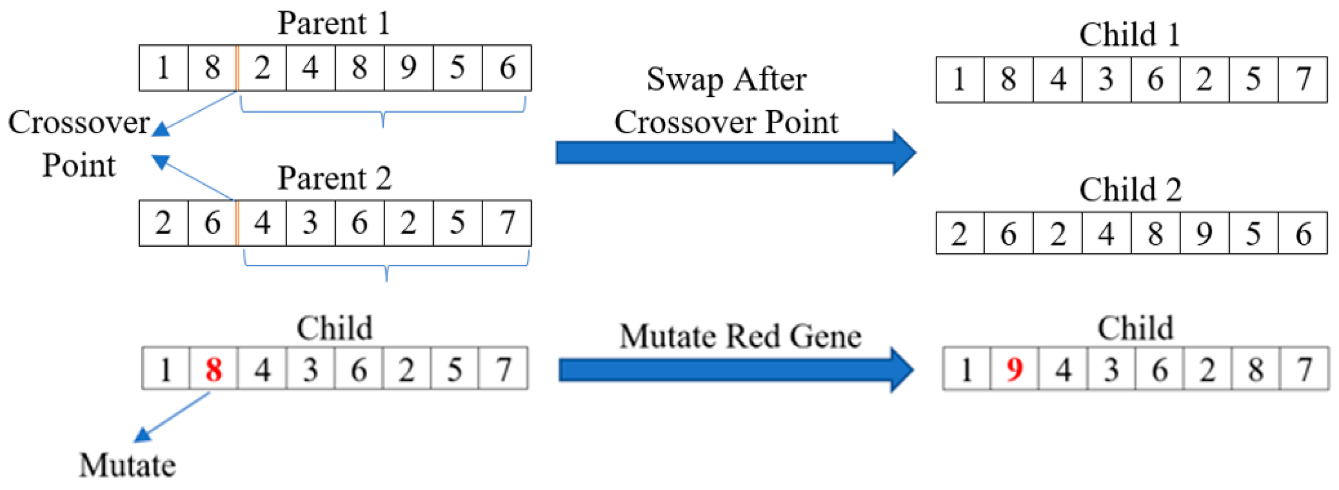
To perform crossover, a random crossover point (index) is selected, and the genes from each parent can be spliced together to create a pair of unique children. Crossover only occurs if a randomly generated number (between 0 and 1) is less than the predefined crossover rate. If crossover should not occur, the children are simply the same as the parents. Then, mutation can be applied to each of the children produced. The mutation operation randomly changes one (or more) gene in each child with respect to the problem constraints. This is performed by iterating over the genes of the children and generating a random number between 0 and 1. If this number is less than the predefined mutation rate, the gene will be mutated. In the literature, the crossover probability is much higher than the mutation probability. This is because the large crossover probability allows for greater exploration of the solution space, while the lower mutation probability allows the solutions to explore the neighboring solutions space more effectively. The crossover and mutation processes can be visualized in Figure 3.

The GA was selected for this research as a means of assigning vehicles to sub-areas and selecting the optimal start point within each sub-area. The objective of the GA was to find the optimal solution that yields the lowest overall traveling time. The overall traveling time can be defined as the longest traveling time out of all operating vehicles. This can be formulated in Equations (9) and (10). In Equation (9), $f$ is the objective function, which is to minimize the overall operation time (maximum operation of all operational vehicles), and $v_n$ is the operation time of vehicle $n$. The vehicle operation time ($v_n$) can be formulated in Equation (10), where $p_j$ is the distance from the last area assigned to vehicle $n$ to the depot, $s_d$ is the deadhead speed, $s_s$ is the servicing speed, $p_i$ is the distance from the vehicle to the starting point of the next service area $i$, $d_i$ is the distance of the servicing path in sub-area $i$, and $p_k$ is the distance from the point where a constraint is violated to the depot. $p_k$ is multiplied by 2 since the vehicle needs to go to the depot and back when a constraint (water or debris capacity) is violated. When $i=0$, $p_i$ is the distance from the depot to the starting point of the first sub-area. All distances were calculated using the A* shortest path algorithm [41].

The objective function can be modified to improve the workload balance, minimize distance, or any other quantifiable metric. However, it was found from experimentation that the overall servicing time minimization yielded the best results.

$$f=\min \left\{\max \{v_1,\dots ,v_n\}\right\}$$

(9)

$$v_n=\frac{p_j}{s_d}+{\sum }_{i=0}^j\left(\frac{p_i}{s_d}+\frac{d_i}{s_s}\right)+{\sum }_{k=0}^l\frac{{2p}_k}{s_d}$$

(10)

2.3. Real-Time Scheduling

When the higher-level path generation algorithm is executed, the paths for each vehicle are planned based on the initial conditions. Typically, each vehicle begins at the depot with a full water tank, empty debris tank, and full battery. However, the algorithm can provide optimal solutions based on the input conditions if they differ from the expected ones. For example, the vehicles’ starting locations may differ from the depot, which will result in different paths.

This concept can be extended to the real-time scheduling aspect of this study. Specifically, when a vehicle becomes out of service (due to an unexpected breakdown), the portion of the path that has already been serviced does not need to be serviced again by the remaining vehicles. So, each vehicle should be keeping a record of the originally planned path and the portion of that path that has been serviced already. When a breakdown occurs for one of the vehicles, the higher-level path generation algorithm can be executed again with the portion of the graph that has not yet been serviced. To do this, the edges that have been serviced in each sub-area can be removed from the higher-level graph, and the lower-level paths can be updated with new starting point(s) that are dependent on how much of the sub-area has been serviced before the breakdown. A graphical example of this can be found in Figure 4, where the same concept can be extended to all sub-areas in the higher-level graph.

3. Problem Specific Parameters for Uchi Park Zoo

In this section, the problem-specific parameters (for the case study in Uchi Park), the graph generation methods, and the application of the proposed route optimization methodology will be discussed in detail.

3.1. Vehicle and Park Specific Parameters

Uchi Park is equipped with a fleet of 2 identical autonomous street sweepers. The sweepers have a width of 1.295 m and a length of 3.810 m; all other dimensions can be seen in Figure 5. Additionally, the vehicle parameters can be seen in

Table 1. Vehicle parameters.

Parameter	Value
Driving Speed (Servicing)	3 km/h
Driving Speed (Deadhead)	8 km/h
Debris Tank Capacity	240 L
Debris Collection Rate *	133.33 L/km
Water Tank Capacity	150 L
Water Distribution Rate *	16.67 L/km
Batter Capacity	40 kWh
Battery Drainage Rate (Servicing)	8 kW
Battery Drainage Rate (Deadhead)	5 kW

* Parameters that are situational dependent.

. In Table 1, some parameters are situation-specific. For example, the debris collection rate and water collection rate are variables and can be set based on debris conditions in the park. These values are rough estimates that were calculated using historical data, a common approach seen in the capacitated arc routing problem (CARP) model with relatively static routes [42]. All variable parameters are denoted with an asterisk in Table 1.

Uchi Park consists of 18 serviceable sub-areas. Some of these are roads (ring roads) that circle the perimeter of the park, and others are paths leading to cages for various animals at the zoo. An aerial view of Uchi Park can be seen in Figure 6. The 18 sub-areas were predefined by Uchi Park to be used as inputs to the algorithm. This provides the freedom to select which set of sub-areas are to be serviced.

3.2. Lower-Level Graph Generation

Raw data for Uchi Park were provided in the form of a set of coordinates for each of the predefined sub-areas. However, the serviceable area within each boundary needs to be converted into a graph so the developed routing algorithms can compute optimal coverage paths. This is called the lower-level graph generation. To do this, an offset method that is dependent on the outer boundary of the sub-area is proposed.

Using the buffer function provided by the Shapely Python library [43], serviceable tracks can be continuously generated by offsetting the outer boundary of the sub-area inwards with respect to the vehicle width. The boundary can be continuously offset until the new boundary’s perimeter is less than 10 m. 10 m was selected as the threshold, which is based on the vehicle length. Since the vehicle is approximately 4 m long, it should be able to service a loop that is at least twice the length of the vehicle. So, 10 m (slightly larger than twice the vehicle length) was selected as the minimum length of an offset boundary for the lower-graph generation. The static obstacles (buildings and animal cages) within the sub-areas should be removed before the offset method is applied so edges that collide with them are not created. As seen in Figure 7, there is a hole in the area, which represents a static obstacle. Each time the boundary is offset inwards, another serviceable ring is created; this is called a layer route. The shape of the layer routes is dependent on the geometry of the sub-area.

Several other methods were considered for the lower-level graph generation, such as a grid-based approach, but the offset method yielded comparatively smoother serviceable edges. Additionally, the offset method guarantees full area coverage (over 94%) for all sub-areas. A graphical representation of the layer routes created by the offset method can be seen in Figure 7. In Figure 7, each color ring corresponds to a layer route created by offsetting the outer boundary (perimeter) inwards. The perpendicular distance between each layer route is proportional to the vehicle width, and the smallest layer route has a length that exceeds the 10 m threshold.

After applying the offset method, all layer routes are initially disconnected. To create a graph, edges should be added to connect each layer route. A search algorithm was developed for this task to ensure that each point on the layer routes is connected to a meaningful set of points (nearest points on adjacent layer routes). The connections that are made in this process are unserviceable edges since the vehicle width covers the area between each layer route. Some examples of the completed lower-level graph can be seen in Figure 8. In Figure 8, the black edges are created by offsetting the perimeter of the sub-area inwards, while the red edges correspond to the connections made between each layer route. As seen in Figure 8, the connections between each layer route (red edges) are joined by the nearest points on the adjacent layer routes. The connections between the layer routes allow for minimum distance deadhead traveling between serviceable edges. Additionally, the deadhead connections are used as required to reach other serviceable edges; thus, only a subset of them may be used.

3.3. Higher-Level Graph Generation

The higher-level graph is the “total graph” that connects the lower-level graphs together. Without the higher-level graph connections, each lower-level graph is isolated, and a path between each lower-level graph cannot be found. Creating the connections to make the higher-level graph makes all lower-level graphs strongly connected, so a path exists connecting any pair of nodes.

To make such connections, a search algorithm was developed. Initially, all lower-level graphs are isolated from each other, but they are geographically very close to each other. The developed search algorithm explores the possible connections for all nodes in adjacent sub-areas. First, adjacent sub-areas are identified by offsetting two target sub-areas outwards using the Shapely buffer function [43], then checking to see if the resulting buffers overlap. If they overlap, this means that the two target sub-areas are adjacent. Then, all nodes from the two target sub-areas can be joined with an edge, and the edges below a specified threshold are kept as the connecting edges. For this case, the threshold was set to 2.0 m (slightly above the vehicle width). Adding the connections can be graphically seen in Figure 9, where the highlighted edges are connections that were added manually to create the higher-level graph. As seen in Figure 5, the connections made join adjacent sub-areas by placing an edge in the blank space between the sub-areas.

As seen in Figure 9, the highlighted connections are in the most logically correct locations. Meaning that each added edge connects a node from one lower-level graph to the nearest node in an adjacent lower-level graph. After creating the connections between each lower-level graph, the higher-level graph is completed. A graphical representation of the higher-level graph can be seen in Figure 10. Since the higher-level graph is strongly connected, the A* algorithm can be used to compute the shortest path between any pair of nodes in the network.

3.4. Using the Lower-Level Path Generation

The lower-level path generation should be executed several times (once for each starting point) for each sub-area. The starting points are the nodes that were used to connect adjacent sub-areas. As explained in Section 3.3, edges were added to connect the sub-areas together to create the higher-level graph. The nodes in the connecting edges are used as the starting points for each respective sub-area. So, each sub-area can have several possible starting points. This results in several servicing paths that are dependent on the starting point selected. The optimal start point is determined in the higher-level path generation and is dependent upon the sub-areas assigned to each vehicle, the vehicle location, and the vehicle constraints. It should be mentioned that a lower-level path generation is a pre-processing event that does not occur in real-time. Additionally, the SSN algorithm is applied to each sub-area as many times as there are starting points. This further increases the computation time since the algorithm needs to be executed several times for each sub-area. As a result, all lower-level paths should be computed before using the higher-level path generation.

3.5. Using the Higher-Level Path Generation

The chromosome structure needs to reflect the sub-area assigned to each vehicle, the order of operation, and the sub-area starting point. This means that each sub-area should only appear once in the chromosome, while each vehicle should appear at least once. The chromosome structure can be seen in Figure 11.

As previously stated, the crossover operation splices the genes from 2 different parents together to create a pair of children. However, the crossover point cannot be any index in the chromosome structure. This is because crossover is used to change the order of operation for servicing sub-areas. Additionally, the starting points for each sub-area should be associated with the corresponding sub-area. Because of this, preserving the vehicle + sub-area + sub-area starting point is desired. To do so, the introduction of “chromosome blocks” is proposed. A chromosome block is used to group every three genes in the chromosome together such that the desired genes cannot be separated. Instead of performing the crossover at any random index, the crossover point should be selected at an index that preserves the chromosome blocks. An example of the chromosome block structure and the candidate crossover points can be seen in Figure 12.

Similarly, mutation cannot occur on any random gene. Since the purpose of mutation is to explore the neighboring solutions, only small changes should be applied to the chromosome. As such, two mutation operators are proposed: vehicle mutation and start point mutation. Additionally, mutation should occur only once per chromosome block to prevent redundant solution space exploration. If mutation should occur in the chromosome block, there is a 50/50 chance of applying vehicle mutation or starting point mutation. The proposed mutation scheme can be visualized in Figure 13.

Since the higher-level path generation uses the pre-processed results generated by the lower-level path generation, the GA can select the optimal start point for each sub-area such that the overall travel time is minimized. Additionally, the GA is responsible for managing the debris and water tank levels. Based on the input parameters (debris and water rate), the GA can predict when the vehicle should make a depot trip to dump debris or refill the water tank. In these cases, the vehicle travels from the point where the constraint is violated to the depot and then back carries on the path as expected.

As seen in the literature, the typical process for multi-vehicle coverage begins with dividing the area into several sub-areas, and then the paths are generated in each sub-area. In the proposed approach, several paths are pre-processed in predetermined sub-areas. The main benefit of this approach is that pre-processing can save computation time in the GA, and several candidate paths are calculated with different starting and ending points. The GA can then select the optimal starting/ending point pair that yields the least total distance. Since each starting point has a predetermined ending point, the starting point has a direct influence on the total distance since the vehicle will need to travel from one sub-area to the next. In the traditional case, the paths are to be calculated after dividing them amongst a fleet of vehicles, which requires additional computation time and typically has a fixed starting and ending point pair that can result in increased distance.

Additionally, the GA penalizes solutions where the battery constraint for any vehicle is violated. As highlighted in Table 1, different battery drainage rates are applied based on the vehicle’s status (servicing or deadheading). When any of the vehicle’s battery constraints are violated, a large penalty is applied to exclude these solutions from the evolutionary pool. This is because charging the battery takes too long in real-time applications, and solutions should be provided so that the battery for all vehicles does not drain. This is an emerging topic in routing applications that requires special attention [44]. A case where the battery constraint is violated can be when most of the sub-areas are assigned to a vehicle, while the remaining vehicles only service one sub-area each. It should be noted that the entire park cannot be serviced by only one vehicle, and thus multiple should be used.

The higher-level path generation can also handle breakdown conditions. In these cases, the remainder of the path assigned to the broken vehicle can be redistributed amongst the in-service vehicles. The GA will have to be executed again to generate the new paths. This results in routes that may differ from the originally planned ones (from the non-breakdown case).

4. Results and Discussion

Two test case scenarios were used to evaluate the performance of the proposed algorithms. The first scenario consists of two vehicles operating under normal conditions, while the second scenario consists of a vehicle breaking down during operations. The statistics for each case will be presented and analyzed with the objective of validating the proposed methods. All results presented in this section are based on simulated experiments which are used to validate the proposed methodology. This technology has not been applied in real-world scenarios yet.

The same parameters for the higher-level path generation algorithm were used for both scenarios. They can be seen in

Table 2. Higher-level GA parameters used for both test scenarios.

Parameter	Value
Generations	60
Population Size	20
Crossover Probability	0.90
Mutation Probability	0.05
Processors *	5

* Parameters that are specifically for parallel computing.

. As seen in Table 2, several processors can be used for parallel computing. This means that the population can be divided into chunks and distributed to each processor to be calculated in parallel. From experimentation, the optimal number of processors was found to be five since additional time needs to be allocated for the work division amongst the processors. Furthermore, the variables in Table 1 were used during optimization and to calculate the statistics.

4.1. Scenario 1: 2 Normal Vehicles

A summary of the normal scenario can be found in

Table 3. Statistics for the normal scenario. In this case, both vehicles operate as expected without any breakdown.

Vehicle	1	2
Total Distance	10,783.4 m	11,334.7 m
Total Time	3 h 49 min 48 s	3 h 52 min 48 s
Service Distance	6836.3 m	6272.9 m
Service Time	2 h 16 min 48 s	2 h 5 min 24 s
Deadhead Distance	2384.0 m	3022.2 m
Deadhead Time	0 h 18 min 0 s	0 h 22 min 48 s
Depot Trip Distance	1563.1 m	2039.6 m
Depot Trip Time	0 h 12 min 0 s	0 h 15 min 0 s
Time Penalty	1 h 3 min 36 s	1 h 9 min 36 s
Depot Trips 1	3	3
Total Distance Efficiency 2	59.27%
Total Time Efficiency 3	82.59%
Total Coverage Ratio 4	99.23%

¹ This is the total number of times each vehicle requires a trip to the depot to dump debris and refill water. ² Defined as the serviceable distance divided by the total distance. ³ Defined as the servicing time divided by the total travel time. 90% of the time penalty is allocated to servicing. ⁴ Defined as the total area coverage for all vehicles.

. In Table 3, the time penalty is applied to the total path generated in accordance with Equation (2). Since the servicing paths created by the lower-level path generation approach consist of many turns, most of the time, a penalty is applied to the service route. Specifically, this was assumed to be 90% since deadheading was a comparatively simple and less time-consuming operation. Additionally, the lower-level paths are more complicated since the layer routes are dependent on the geometry of the sub-areas, which can be complex (creating many turns). This means that more time is allocated to servicing than deadheading, which results in a higher time-based efficiency than distance-based efficiency. Additionally, the servicing speed is less than the deadhead speed, so there will naturally be more time allocated to servicing than deadheading, resulting in a greater difference between the time-based efficiency and the distance-based efficiency. A graphical representation of the sub-area traversal sequence can be seen in Figure 14 for the normal scenario.

4.2. Scenario 2: 1 Normal Vehicle with 1 Breakdown Vehicle

A breakdown scenario was proposed to evaluate the performance of the real-time scheduling aspect of the algorithm. In this scenario, the remainder of the path left by the broken vehicle can be redistributed to the active vehicle(s). So, a simulated breakdown was created for vehicle 2 after traveling 8 km. A summary of the normal scenario can be found in

Table 4. Statistics for the breakdown scenario. In this case, vehicle 2 breaks down while vehicle 1 remains in service.

Vehicle	1	2
Total Distance	13,925.5 m	8007.4 m
Total Time	4 h 51 min 36 s	2 h 50 min 24 s
Service Distance	8483.3 m	4624.1 m
Service Time	2 h 49 min 48 s	1 h 32 min 24 s
Deadhead Distance	3492.7 m	2294.9 m
Deadhead Time	0 h 26 min 24 s	0 h 17 min 24 s
Depot Trip Distance	1949.5 m	1088.4 m
Depot Trip Time	0 h 14 min 24 s	0 h 8 min 24 s
Time Penalty	1 h 21 min 36 s	0 h 52 min 48 s
Depot Trips 1	4	2
Total Distance Efficiency 2	59.76%
Total Time Efficiency 3	82.94%
Total Coverage Ratio 4	99.23%

¹ This is the total number of times each vehicle requires a trip to the depot to dump debris and refill water. ² Defined as the serviceable distance divided by the total distance. ³ Defined as the servicing time divided by the total travel time. 90% of the time penalty is allocated to servicing. ⁴ Defined as the total area coverage for all vehicles.

. Like the normal scenario, the same trend is seen for distance and time efficiency (time efficiency is much higher) because of the slower servicing speed and time penalty applied for sharp turns while servicing. A graphical representation of the sub-area traversal sequence for the breakdown scenario can be seen in Figure 15. In Figure 15b, the location of the second vehicle breakdown is shown, and the remainder of that sub-area is assigned to the first vehicle.

As expected, the overall operation time (maximum travel time) was higher for the breakdown condition since vehicle 1 was assigned more sub-areas after vehicle 2 broke down. Specifically, the operation time increased by approximately 1 h because of this. Additionally, each vehicle is required to do three depot trips in the normal scenario, whereas vehicle 2 breaks down after performing two depot trips, and vehicle 1 must do four depot trips because of the increased sub-area servicing. In both scenarios, the respective efficiencies (time efficiency and distance efficiency) remain almost constant. This highlights the performance of the algorithm’s real-time scheduling capabilities for the breakdown scenario. This also confirms that the proposed algorithm can be used to yield optimal solutions in any scenario for a fleet of vehicles.

4.3. Computation Time, Area Coverage, and Work Efficiency

To ensure that the proposed algorithms can perform in real time, an analysis of the computation time should be conducted. In

Table 5. Runtime comparison for different scenarios and conditions.

Scenario	Generations (In the GA)	Runtime (s)
2 Vehicles—Complete	60	170
1 + 1 Vehicles—Breakdown	60	19
2 Vehicles—Complete	30	85
1 + 1 Vehicles—Breakdown	30	13
2 Vehicles—Complete	3	16
1 + 1 Vehicles—Breakdown	3	6

, a summary of the computation time for different scenarios and conditions can be seen. Specifically, the computation time for several different generations in the GA and the two mentioned scenarios (two normal vehicles and the breakdown scenario) is highlighted. As seen in Table 5, the runtime increases with more generations. This trend is seen for both scenarios. Increasing the generations (allowing the solutions to evolve more) means that a higher quality solution will be produced at the expense of a longer computation time. However, experimentation shows that little improvement is made to the overall travel time using more generations, thus leading to the conclusion that fewer generations can be used to apply the proposed methods in real time. For the results presented in this paper, 60 generations were used for the GA since the experiments were conducted offline. In real-time applications, it is recommended to use three generations since there are no significant improvements made to the solutions that can justify the extended computation times. Additionally, in any number of generations, the GA cannot guarantee that the global optimum has been found. It can only be assumed that an acceptable local optimum has been found due to the complexity of the problem.

Another metric used to highlight the performance of real-time scheduling is work efficiency. The work efficiency can be formulated in Equation (11). Ideally, this number should be near 100%, but it is also dependent on where the breakdown occurs. In this study, vehicle 2 broke down after traveling 8 km, which yields a work efficiency of 79.8%. However, if the vehicle were to break down earlier, the work efficiency would decrease since the remaining vehicle would service more sub-areas.

$$work efficiency=\frac{overall travel time for the normal scenario}{overall travel time for the breakdown scenario}$$

(11)

Another method of quantifying real-time scheduling can be defined. This is called recovery efficiency, and it can be formulated in Equation (12). The recovery efficiency quantifies how optimal the breakdown paths are in comparison to the paths planned for the normal scenario. If this is 100%, this means that the proposed methods can schedule paths that are of the same quality as the originally planned paths. The recovery efficiency was calculated to be 100.1%. Having such a high recovery efficiency means that the proposed methods can create paths that are comparable to the ones originally planned.

$$recovery efficiency=\frac{total travel time for the normal scenario}{total travel time for the breakdown scenario}$$

(12)

Since the lower-level path generation is used to pre-process the service paths for each sub-area, the area coverage remains the same for any scenario and is independent of the performance of the higher-level path generation. The area coverage for each sub-area can be seen in

Table 6. Area coverage percentage for each sub-area.

Area	Coverage Ratio (%)
lane_1	99.99
lane_2	99.72
lane_3	99.98
lane_4	99.99
lane_5	99.62
lane_6	100.00
lane_7	100.00
lane_8	94.26
lane_9	99.97
lane_10	99.91
lane_11	99.54
lane_12	96.83
lane_13	99.86
node_1	99.73
node_2	99.35
node_3	99.74
node_4	97.62
node_5	99.98
Average	99.23

, where all sub-area coverages are over 94%, and the average area coverage is 99.23%. Having such high area coverage rates validates the performance of the lower-level path generation methods (SSN) for the street-sweeping application.

It should also be mentioned that using a lower and higher-level path generation approach is something that has seen little to no consideration in existing studies. As a result, a direct comparison between the methods discussed in this paper and existing studies is not applicable. Instead, the promising results presented in this paper are used to validate the proposed approaches for real-time scheduling of autonomous mobile applications.

5. Conclusions

In this study, a method of generating optimal servicing paths for a fleet of autonomous street sweepers was proposed for a case study in Uchi Park, South Korea. Methods were proposed to convert the serviceable area into a graph-like structure that can be used for optimization methods and graph traversal algorithms. The developed graph generation methods can guarantee an average area coverage rate of over 99.23% for all sub-areas. The proposed path generation algorithms operate on two levels: the lower level and the higher level. The novel SSN path planning method was used on the lower level to generate optimal service routes in each sub-area, while a modified GA was applied on the higher level to schedule the fleet and manage the vehicle constraints. The proposed methods were validated using two scenarios: the normal scenario and the breakdown scenario. The recovery efficiency shows that the routes produced after a breakdown share similar statistics, thus validating the proposed methodology for real-time applications. Additionally, the proposed methodology improves existing multi-robot scheduling by considering several complex constraints (specific to street-sweeping) that have not been explored in the literature. The methodology discussed in this paper can be applied to many other scheduling and routing applications and is not limited to the case study in Uchi Park. Specifically, the proposed methodology can be applied to any real-time multi-robot (or multi-vehicle) CARPs with a fixed set of required edges. Since the mentioned methods have been applied to street-sweeping, it is confirmed that many constraints (battery, water, and debris capacity) can be handled simultaneously. This concludes that the same approach can be applied to real-time multi-robot CARPs with the same number (or less) constraints. An example of this can be waste collection, where several vehicles can be dispatched from a single depot to collect curbside waste. The higher-level approach can handle many vehicles; however, it was only tested with two. This was performed to mimic the expected conditions in Uchi Park since they only have two autonomous street sweepers.

Limitations to this study include the runtime and turn radius. Since the quality of the solution and runtime increase proportional to the number of generations, low generations for real-time applications cannot guarantee near-optimal solutions. Methods were taken to try to reduce the computation time (parallel computing and storing repeated paths); however, it is still relatively high for real-time applications. Additionally, the vehicle turn radius was not considered for this study. This means that the paths generated using the proposed methods contain sharp turns that cannot be achieved because of the turn radius constraint. Another target for future studies can include simulations and real-world applications. In this study, the methods used to generate the routes were validated, but the lack of physical experiments with the generated routes leaves room for further research. When experimenting in real-world scenarios, the local path planner onboard the vehicles will be instructed to follow the global paths generated by the proposed methodology, and the routes will be distributed to the vehicles wirelessly as required. This was not within the scope of the research presented in this paper since only the static obstacles were considered. As a result, additional research would be required to implement the path-tracking control technology with dynamic obstacle avoidance and trajectory recovery.

References

1. Viet, H.H.; Dang, V.H.; Laskar, M.N.U.; Chung, T. BA: An online complete coverage algorithm for cleaning robots. Appl. Intell. 2013, 39, 217–235. [Google Scholar] [CrossRef]
2. Hasan, K.M.; Al-Nahid, A.; Reza, K.J. Path planning algorithm development for autonomous vacuum cleaner robots. In Proceedings of the 3rd International Conference on Informatics, Electronics & Vision, Dhaka, Bangladesh, 23–24 May 2014. [Google Scholar]
3. Hameed, I.A. Coverage path planning software for autonomous robotic lawn mower using Dubins’ curve. In Proceedings of the 2017 IEEE International Conference on Real-time Computing and Robotics, Okinawa, Japan, 14–18 July 2017. [Google Scholar]
4. Wang, T.; Huang, P.; Dong, G. Modeling and path planning for persistent surveillance by unmanned ground vehicle. IEEE Trans. Autom. Sci. Eng. 2021, 18, 1615–1625. [Google Scholar] [CrossRef]
5. Parsons, T.; Hanafi Sheikhha, F.; Ahmadi Khiyavi, O.; Seo, J.; Kim, W.; Lee, S. Optimal path generation with obstacle avoidance and subfield connection for an autonomous tractor. Agriculture 2022, 13, 56. [Google Scholar] [CrossRef]
6. Yang, N.; Zhang, W.; Yu, W. Coverage path planning for autonomous road sweepers in obstacle-cluttered environments. In Proceedings of the 2022 IEEE Conference on Control Technology and Applications, Trieste, Italy, 22–25 August 2022. [Google Scholar]
7. Gonzalez-de-Santos, P.; Ribeiro, A.; Fernandez-Quintanilla, C.; Lopez-Granados, F.; Brandstoetter, M.; Tomic, S.; Pedrazzi, S.; Peruzzi, A.; Pajares, G.; Kaplanis, G.; et al. Fleets of robots for environmentally-safe pest control in agriculture. Precision Agric. 2017, 18, 574–614. [Google Scholar] [CrossRef]
8. Bautin, A.; Simonin, O.; Charpillet, F. Towards a communication free coordination for multi-robot exploration. In Proceedings of the 6th National Conference on Control Architectures of Robots, Grenoble, France, 24–25 May 2011. [Google Scholar]
9. Oksanen, T.; Visala, A. Coverage path planning algorithms for agricultural field machines. J. F. Robot. 2009, 26, 651–668. [Google Scholar] [CrossRef]
10. Current, J.R.; Schilling, D.A. The covering salesman problem. Transp. Sci. 1989, 23, 208–213. [Google Scholar] [CrossRef]
11. Wang, Z.; Bo, Z. Coverage path planning for mobile robot based on genetic algorithm. In Proceedings of the IEEE Workshop on Electronics, Computer and Applications, Ottawa, Canada, 8–9 May 2014. [Google Scholar]
12. Pratama, P.S.; Kim, J.W.; Kim, H.K.; Yoon, S.M.; Yeu, T.K.; Hong, S.; Oh, S.J.; Kim, S.B. Path planning algorithm to minimize an overlapped path and turning number for an underwater mining robot. In Proceedings of the 15th International Conference on Control, Automation and Systems, Busan, Republic of Korea, 13–16 October 2015. [Google Scholar]
13. Cabreira, T.M.; Brisolara, L.B.; Ferreira Paulo, R. Survey on coverage path planning with unmanned aerial vehicles. Drones 2019, 3, 4. [Google Scholar] [CrossRef]
14. Chakraborty, S.; Elangovan, D.; Govindarajan, P.L.; ELnaggar, M.F.; Alrashed, M.M.; Kamel, S. A comprehensive review of path planning for agricultural ground robots. Sustainability 2022, 14, 9156. [Google Scholar] [CrossRef]
15. Nakamura, Y.; Sekiguchi, A. The chaotic mobile robot. IEEE Trans. Robot. Autom. 2001, 17, 898–904. [Google Scholar] [CrossRef]
16. Hong Li, C.; Fang, C.; Ying Wang, F.; Xia, B.; Song, Y. Complete coverage path planning for an Arnold system based mobile robot to perform specific types of missions. Front. Inform. Technol. Electron. Eng. 2019, 20, 1530–1542. [Google Scholar]
17. Volos, C.K.; Kyprianidis, I.M.; Stouboulos, I.N.; Nistazakis, H.E.; Tombras, G.S. Cooperation of autonomous mobile robots for surveillance missions based on hyperchaos synchronization. J. App. Math. Biol. 2016, 6, 125–143. [Google Scholar]
18. Hwan Kang, K.; Hoon Lee, Y.; Ki Lee, B. An exact algorithm for multi depot and multi period vehicle scheduling problem. In Computational Science and Its Applications–ICCSA 2005; Gervasi, O., Gavrilova, L.M., Kumar, V., Lagana, A., Lee, H.P., Mun, Y., Taniar, D., Tan, C.J.K., Eds.; Springer: Berlin/Heidelberg, Germany, 2005; Volume 3483, pp. 350–359. [Google Scholar]
19. Liu, Y.; Lin, X.; Zhu, S. Combined coverage path planning for autonomous cleaning robots in unstructured environments. In Proceedings of the World Congress on Intelligent Control and Automation, Chongqing, China, 25–27 June 2008. [Google Scholar]
20. Turchin, P. Quantitative analysis of movement: Measuring and modeling population redistribution in animals and plants. Q. Rev. Biol. 1999, 74, 240–241. [Google Scholar]
21. Kang, Y.; Shi, D. A research on area coverage algorithm for robotics. In Proceedings of the 2018 IEEE International Conference of Intelligent Robotic and Control Engineering, Lanzhou, China, 18 October 2018. [Google Scholar]
22. Waanders, M. Coverage Path Planning for Mobile Cleaning Robots. Available online: https://api.semanticscholar.org/CorpusID:15584364 (accessed on 14 December 2023).
23. Joshi, P. Artificial Intelligence with Python; Packt Publishing: Birmingham, UK, 2017. [Google Scholar]
24. Kabir, A.M.; Kaipa, K.N.; Marvel, J.; Gupta, S.K. Automated planning for robotic cleaning using multiple setups and oscillatory tool motions. IEEE Trans. Autom. Sci. Eng. 2017, 14, 1364–1377. [Google Scholar] [CrossRef]
25. Barrientos, A.; Colorado, J.; Cerro, J.D.; Martinez, A.; Rossi, C.; Sanz, D.; Valente, J. Aerial remote sensing in agriculture: A practical approach to area coverage and path planning for fleets of mini aerial robots. J. F. Robot. 2011, 28, 667–689. [Google Scholar] [CrossRef]
26. Tan, C.S.; Mohd-Mokhtar, R.; Arshad, M.R. A comprehensive review of coverage path planning in robotics using classical and heuristic algorithms. IEEE Access 2021, 9, 119310–119342. [Google Scholar] [CrossRef]
27. Razali, N.M.; Geraghty, J. Genetic algorithm performance with different selection strategies in solving TSP. In Proceedings of the World Congress on Engineering 2011, London, UK, 6–8 July 2011. [Google Scholar]
28. Hameed, I.A.; Bochtis, D.D.; Sorensen, C.G. Driving angle and track sequence optimization for operational path planning using genetic algorithms. Appl. Eng. Agric. 2011, 27, 1077–1086. [Google Scholar] [CrossRef]
29. Xidias, E.; Zacharia, P.; Nearchou, A. Path planning and scheduling for a fleet of autonomous vehicles. Robotica 2016, 10, 2257–2273. [Google Scholar] [CrossRef]
30. Almadhoun, R.; Taha, T.; Seneviratne, L.; Zweiri, Y. A survey on multi-robot coverage path planning for model reconstruction and mapping. SN Appl. Sci. 2019, 1, 847. [Google Scholar] [CrossRef]
31. Ahmadzadeh, A.; Keller, J.; Pappas, G.; Jadbabaie, A.; Kumar, V. An optimization-based approach to time-critical cooperative surveillance and coverage with UAVs. Springer Tracts. Adv. Robot. 2008, 39, 491–500. [Google Scholar]
32. Maza, I.; Ollero, A. Multiple UAV cooperative searching operation using polygon area decomposition and efficient coverage algorithms. In Distributed Autonomous Robotic Systems 6; Alami, R., Chatila, R., Asama, H., Eds.; Springer: Tokyo, Japan, 2007; pp. 221–230. [Google Scholar]
33. Khaledyan, M.; de Queiroz, M. A formation maneuvering controller for multiple non-holonomic robotic vehicles. Robotica 2018, 37, 189–211. [Google Scholar] [CrossRef]
34. Nfaileh, N.; Alipour, K.; Tarvirdizadeh, B.; Hadi, A. Formation control of multiple wheeled mobile robots based on model predictive control. Robotica 2022, 40, 3178–3213. [Google Scholar] [CrossRef]
35. Sun, D.; Wang, C.; Shang, W.; Feng, G. A synchronization approach to trajectory tracking of multiple mobile robots while maintaining time-varying formations. IEEE Trans. Robot. 2009, 25, 1074–1086. [Google Scholar]
36. Kucharska, E. Dynamic vehicle routing problem—Predictive and unexpected customer availability. Symmetry 2019, 11, 546. [Google Scholar] [CrossRef]
37. Song, J.; Gupta, S.; Hare, J. Game-theoretic cooperative coverage using autonomous vehicles. In Proceedings of the 2014 Oceans, St. John’s, NL, Canada, 14–19 September 2014. [Google Scholar]
38. Song, J.; Gupta, S. CARE: Cooperative autonomy for resilience and efficiency of robot teams for complete coverage of unknown environments under robot failures. Auton. Robot. 2020, 44, 647–671. [Google Scholar] [CrossRef]
39. Sun, R.; Tang, C.; Zheng, J.; Zhou, Y.; Yu, S. Multi-robot path planning for complete coverage with genetic algorithms. In Proceedings of the International Conference on Intelligent Robotics and Applications, Shenyang, China, 8–11 August 2019. [Google Scholar]
40. Holland, J.H. Genetic algorithms and the optimal allocation of trials. SIAM J. Comput. 1973, 2, 88–106. [Google Scholar] [CrossRef]
41. Hart, P.E.; Nilsson, N.J.; Raphael, B. Formal basis for the heuristic determination of minimum cost paths. Syst. Sci. Cybern. 1968, 4, 100–107. [Google Scholar] [CrossRef]
42. Liu, G.; Zhao, H.; Yang, H.; Zhiwei, D.W.; Wang, D. A fleet management system of autonomous electric street sweepers. In Proceedings of the IEEE Conference on Cybernetics and Intelligent Systems, Penang, Malaysia, 9–12 June 2023. [Google Scholar]
43. The Shapely User Manual. Available online: https://shapely.readthedocs.io/en/stable/manual.html (accessed on 16 December 2023).
44. Almouhanna, A.; Quintero-Araujo, C.L.; Panadero, J.; Juan, A.A.; Khosravi, B.; Ouelhadj, D. The location routing problem using electric vehicles with constrained distance. Comp. Oper. Res. 2020, 115, 104864. [Google Scholar] [CrossRef]
Figure 1. The GA process visualized.
Robotics 13 00037 g001
Figure 2. Roulette style parent selection scheme used in the GA. The red arrow represents the randomized selection process mimicking that of a roulette wheel.
Robotics 13 00037 g002
Figure 3. The GA crossover and mutation process visualized. The lists of numbers represent an arbitrary set of genes in a chromosome. In the mutation process, the red gene is selected to undergo mutation, changing it from 8 to 9.
Robotics 13 00037 g003
Figure 4. Example of the start points changing in real-time scheduling due to an unexpected breakdown. The original starting points can be seen in green in (a), and the updated starting points can be seen in red in (b). The updated starting points are dependent on the portion of the sub-area that was serviced before the breakdown (highlighted in yellow).
Robotics 13 00037 g004
Figure 5. Vehicle dimensions. Here, the vehicle width (1.295 m) and length (3.810 m) can be seen. The vehicle width relates to how much of the road can be swept at one time.
Robotics 13 00037 g005
Figure 6. Aerial view of Uchi Park Zoo. The main roads can be seen annotated in yellow, and several key features of the park can be described with text.
Robotics 13 00037 g006
Figure 7. Layer routes are created by the offset method for a sub-area. Each layer route is highlighted in a different color.
Robotics 13 00037 g007
Figure 8. (a,b) show two examples of lower-level graphs created using the offset method. Serviceable edges are highlighted in black, while the deadhead edges used to connect layer routes are highlighted in red.
Robotics 13 00037 g008
Figure 9. Connections made to create the higher-level graph can be seen drawn in red and highlighted in yellow. The connections were added to join each lower-level graph.
Robotics 13 00037 g009
Figure 10. The completed higher-level graph with the depot location circled in red. The edges are coloured black, and the nodes are coloured blue.
Robotics 13 00037 g010
Figure 11. Chromosome structure for the higher-level path generation.
Robotics 13 00037 g011
Figure 12. Chromosome blocks and possible crossover points that can be used to preserve the area, start point, and vehicle assignment.
Robotics 13 00037 g012
Figure 13. Example of applying vehicle and starting point mutation in the chromosome.
Robotics 13 00037 g013
Figure 14. Graphical results showing the order of operation for vehicle 1 in yellow (a) and vehicle 2 in green (b).
Robotics 13 00037 g014
Figure 15. Graphical results showing the order of operation for vehicle 1 in yellow (a) and vehicle 2 in green (b) in the breakdown scenario. In this case, vehicle 2 breaks down (the breakdown location can be seen in (b)).
Robotics 13 00037 g015