A Control Interface for Autonomous Positioning of Magnetically Actuated Spheres Using an Artificial Neural Network

Abstract

Electromagnet arrays show significant potential in the untethered guidance of particles, devices, and eventually robots. However, complications in obtaining accurate models of electromagnetic fields pose challenges for precision control. Manipulation often requires the reduced-order modeling of physical systems, which may be computationally complex and may still not account for all possible system dynamics. Additionally, control schemes capable of being applied to electromagnet arrays of any configuration may significantly expand the usefulness of any control approach. In this study, we developed a data-driven approach to the magnetic control of a neodymium magnets (NdFeB magnetic sphere) using a simple, highly constrained magnetic actuation architecture. We developed and compared two regression-based schemes for controlling the NdFeB sphere in the workspace of a four-coil array of electromagnets. We obtained averaged submillimeter positional control (0.85 mm) of a NdFeB hard magnetic sphere in a 2D plane using a controller trained using a single-layer, five-input regression neural network with a single hidden layer.

1. Introduction

The magnetic guidance of particles and devices shows potential for untethered manipulation across a range of medical [1] and industrial applications [2]. Specifically, the manipulation and actuation of particles [3], robots [4], and devices [5] in the milli- to micrometer size range hold particular relevance, as these particles may serve as untethered agents capable of remote-controlled action at a distance [6]. Numerous control algorithms have been developed for the magnetic guidance of various devices [7,8] via an assortment of magnetic coil arrays [9]. Detailed physical modeling approaches have been successfully implemented for controlling magnetic particles [10] and magnetic nanofluids [11] using coil arrays. Often, accomplishing such control requires a reduced-order model of a physical system in which particle motion is driven by external fields [12] (e.g., optical [13], electric [14], acoustic [15], or magnetic [16] fields).

Finite element approaches have been used to model the magnetic fields generated by arrays of coils [17], demonstrating the high-fidelity manipulation of magnetic agents [18]. However, such implementations may be computationally complex and may not innately account for all system dynamics such as coil heating, heterogeneities in the sample environment, or other complexities. Here, we introduced a simple, one-layer, five-input regression neural network for controlling a magnetic sphere in a workspace. Artificial neural networks (ANNs) have a long history in DC motor control [19], with early research applying ANNs for the magnetic guidance of surgical devices such as catheters and implanted magnetic devices [20]. Increasingly, ANNs are being implemented to fine tune magnetic manipulation protocols, gaining ever-increasing precision with iterative training. Prior demonstrations indicate that artificial neural networks can be trained to outperform linear multipole electromagnet modeling relying on fundamental physics, particularly in cases in which iron cores demonstrate nonlinear behavior in the presence of varying applied magnetic fields from electromagnets [21]. Using arrays of electromagnets controlled by ANNs, researchers have positioned millimeter-scale neodymium magnet (NdFeB) disc agents in 2D using an eight-coil array [22], generated real-time predictions of motion dynamics on polymer-based soft magnetic manipulators [23], as well as guided helical microswimmers in 3D [24] and through uncharacterized biomimetic environments [25]. Magnetically guided wheeled robots have been controlled using neuro-fuzzy networks [26], and researchers have made significant progress in guiding endoscopy instruments via intelligent controllers [27,28,29]. Recently, artificial neural networks have been combined with proportional resonant differential feed-forward control methods for controlling currents in coil arrays aimed at supplying rotational fields to magnetic robots, demonstrating improved control of the robot’s position and rotation with extremely small error [30]. Previous work using model-free reinforcement learning aimed at teaching a system to guide a needle using arrays of electromagnets [31] or to suspend a magnetic bead in a fluid against the force of gravity [32,33].

These implementations often require complex, deep, multi-input ANNs requiring significant training via expansive training data sets. Here, we applied a single-layer, five-input ANN architecture to a simple four-coil array, demonstrating the manipulation of a magnetic sphere using magnetic gradients, achieved with no prior training or computational modeling. Using a four-coil array, we achieved the ANN-based manipulation of a hard NdFeB magnetic sphere with average submillimeter precision using a protocol trained on the optical observation of random motions of the sphere in response to random current inputs to a randomly selected coil in the array. We demonstrate that the system is capable of following patterns with both sharp asperities (star-shaped pattern), as well as smooth and continuous curves (circle-shaped pattern). We first describe the mapping of the physical system and delineate the forces involved in actuation. We then describe the experimental apparatus and data collection methodology, including localization and tracking of the NdFeB magnetic sphere. In the sections that follow, we describe the preprocessing of the data and the development of two data-driven controllers (surface fitting model and artificial neural network). We then introduce the ANN developed for manipulating the magnetic sphere and briefly describe system integration and deployment via a custom graphical user interface (GUI). Next, we describe our results, detailing the collected sphere position data set and comparing the accuracy of our ANN approach with the accuracy of a surface fitting model approach. We demonstrate controlled motion along two paths (a star-shaped polygon path and a circular path). Finally, we discuss our control findings and provide some details on the GUI response time, as well as the variability in magnetic sphere detection given different lighting conditions.

2. Methods

In this section, we first establish a system model to provide a basis of the forces involved in magnetic manipulation using our system. Then, we describe our experimental apparatus and data collection protocols, including localization approaches for the electromagnet coils and the NdFeB magnetic sphere. Following that, we describe magnetic sphere tracking, data preprocessing, and the development of two data-driven controllers. Finally, we describe system integration and deployment.

2.1. System Model

Here, we introduce the system with a model that covers the relevant forces involved in magnetic manipulation. We consider a mapping the position of the NdFeB sphere in the workspace as can be described by position $\mathbf{p}$, where $\mathbf{p}$∈ ${\mathbb{R}}^3$. Magnetic fields in ${\mathbb{R}}^3$ are generated by currents $\mathit{i}$ (unit, A) running through any electromagnet ${\mathit{N}}_{\mathit{em}}$ surrounding the workspace [34]. Following an established approach [9], we define the magnetic field $\mathbf{B}$ at a given location $\mathbf{p}$ generated by any single coil carrying current $i$ as $\mathbf{B}(\mathbf{p},\mathit{i})$, where

$$\mathbf{B}(\mathbf{p},\mathit{i})=\int {\mu }_0\frac{\mathit{i}\mathrm{d}\mathbf{l}\times (\mathbf{p}-{\mathbf{p}}_{\mathrm{d}\mathbf{l}})}{{4\pi \parallel \mathbf{p}-{\mathbf{p}}_{\mathrm{d}\mathbf{l}}\parallel }^3}$$

(1)

where $\mathrm{d}\mathbf{l}$ is a differential length (unit, m) of the conductor at a specific location ${\mathbf{p}}_{\mathrm{d}\mathbf{l}}$. Assuming ${\mathit{N}}_{\mathit{em}}$ electromagnets have air cores, we consider the system using a linear magnetic model that follows the principle of superposition, allowing us to write the magnetic field $\mathbf{B}$ for position $\mathbf{p}$ as

$$\mathbf{B}\left(\mathbf{p}\right)=\sum _{k=1}^{N_{em}}{\mathbf{B}}_{\mathbf{k}}\left(\mathbf{p}\right){\mathit{i}}_{\mathit{k}}$$

(2)

where $i_k$ is the current (unit, A) supplied to the $k^{\mathrm{th}}$ coil. Here, we denote the centroid of the position of the magnetic sphere by $\mathbf{p}={[x,y]}^T$. For a NdFeB magnetic sphere having a magnetic moment of ${\mathbf{m}}_{\mathbf{p}}$, the magnetic field $\mathbf{B}\left(\mathbf{p}\right)$ applies a force ${\mathbf{F}}_{\mathbf{m}}$ on the magnetic sphere that is proportional to the magnetic field and field gradient, as given by

$${\mathbf{F}}_{\mathbf{m}}=\nabla ({\mathbf{m}}_{\mathbf{p}}·\mathbf{B}),$$

(3)

and all translational motion generated on the magnetic sphere is induced by magnetic field gradients. Accordingly, we denote the linear velocity of the magnetic sphere with

$$\dot{\mathbf{p}}={[\dot{x},\dot{y}]}^T,$$

(4)

and the acceleration by

$$\ddot{\mathbf{p}}={[\ddot{x},\ddot{y}]}^T.$$

(5)

Here, in addition to the applied magnetic force (${\mathbf{F}}_{\mathbf{m}}$), there are additional forces including the the buoyancy force (${\mathbf{F}}_{\mathbf{b}}$), gravitational force (${\mathbf{F}}_{\mathbf{g}}$), friction force (${\mathbf{F}}_{\mathbf{f}}$), and fluidic drag force (${\mathbf{F}}_{\mathbf{d}}$). Similarly, magnetic fields induce torques on the magnetic sphere, given by ${\tau }_m$, where

$${\tau }_m={\mathbf{m}}_{\mathbf{p}}\times \mathbf{B},$$

(6)

as well as the associated drag torque (${\tau }_{\mathrm{d}}$), and friction torque (${\tau }_{\mathrm{f}}$). Numerous works have presented detailed control approaches for the magnetic manipulation of various magnetic agents, and reviews have covered this topic [7,8]. Here, we bypassed all model-based approaches to magnetic agent control and instead developed two regression-based approaches that do not rely on a priori assessments of coils generating magnetic fields in the presence of magnetic objects.

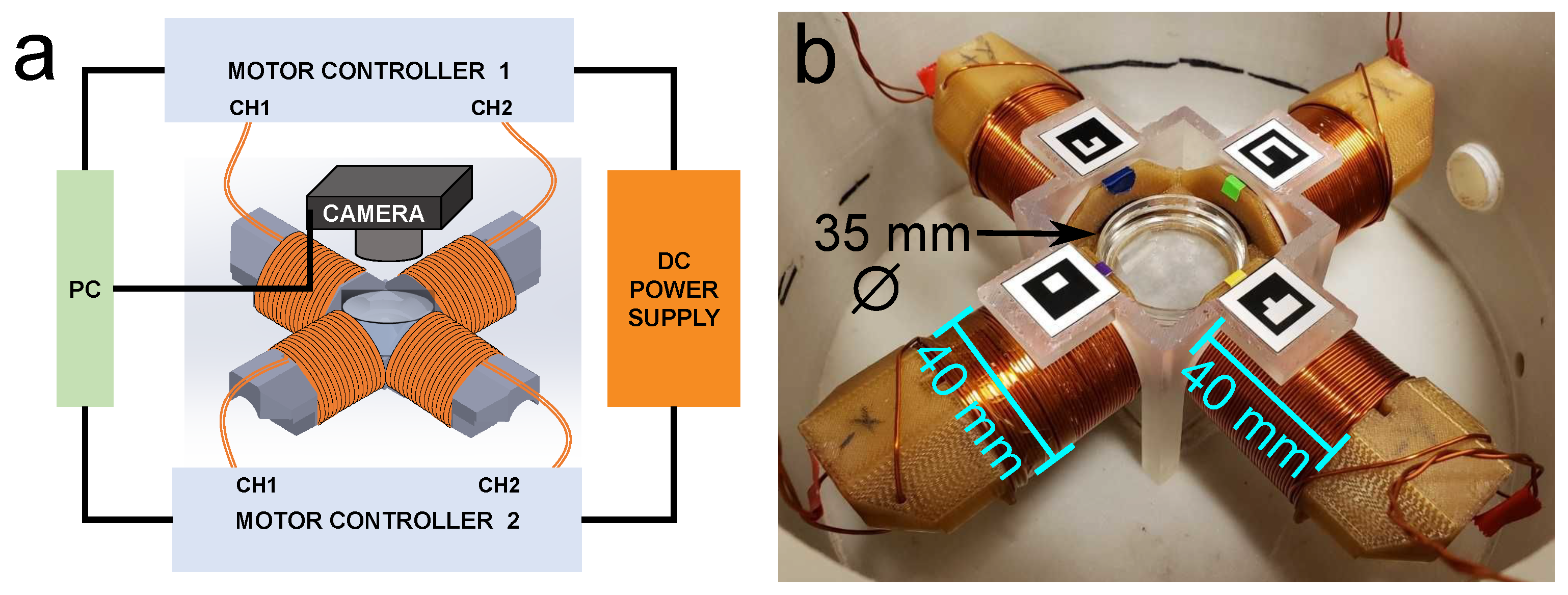
2.2. Experimental Apparatus

Our actuation array consisted of four electromagnets (EMs) positioned in a plane (X–Y plane) and oriented such that coils sat along the cardinal directions (Figure 1a). Opposing EM faces were 40 mm apart, and each EM had an outer diameter of 40 mm, an inner diameter of 22 mm, and a length of 40 mm. Magnets contained 14 layers of windings with 29 turns per layer (AWG 16 magnet wire). We used 3D-printed forms (ULTEM 1010, Stratasys Direct, Rehovot, Israel) to wind the EMs, and iron cores (19 mm diameter, 40 mm length) were placed inside the EMs to increase the fields and gradients generated by the system (Figure 1b).

Magnetic fields were generated via PWM signals supplied by two dual-channel motor controllers (RoboClaw, Basicmicro Motion Control, Temecula, CA, USA) (Figure 1a). Motor controllers were powered by 60VDC AC/DC converters (CUI Inc., Tualatin, OR, USA); EMs were controlled by a computer that generated either random current pulses for training or controlled specific current pulses for prescribed planned object manipulation. All training and experimental manipulations were performed in polycarbonate Petri dishes 35 mm in diameter and 10 mm tall (Falcon 351008, Becton Dickinson Labware, Dubai, United Arab Emirates). The Petri dish was filled with hand sanitizer, and the magnetic sphere was placed in the hand sanitizer for manipulation. A camera (Ipevo Ziggi USB Camera, Ipevo Inc., Taipei, Taiwan) was placed above the petri dish to acquire video frames that were streamed to the PC. The video frames recorded the movement of the magnetic sphere over time. Here, we chose a simple 4.8 mm diameter NdFeB magnetic sphere (K&J Magnetics, Pipersville, PA, USA, product # S3, grade N42). Motor controllers were connected to a computer and graphical user interface (GUI) via USB and controlled using packet serial methods based on a C# library. The simultaneous control of the two motor controllers was accomplished via multithreading handled by the GUI.

2.3. Data Collection

An automated data collection process was implemented in which random currents were supplied to the coils sequentially, and the response of the magnetic sphere was recorded. A diagram of the data collection procedure is shown in Figure 2. During data collection, only one coil was ever activated at a given time to produce one data point on the relationship between that coil activation and the resultant magnetic sphere movement. The single-coil actuation constraint significantly simplified the data collection process but also generated an artificially bounded, artificially simple training dataset. Data collection started by determining the position of the magnetic sphere and recording the sphere’s starting position (Figure 2A). The protocol then determined the distance between the magnetic sphere and any of the four coils. If the magnetic sphere was within 20 mm of a given coil (Figure 2B), the protocol algorithm automatically selected the opposing coil (Figure 2C). For locations more than 20 mm from any coil, the data collection algorithm selected a coil at random for actuation (Figure 2D). The selected coil was activated with a random current scale value, which was recorded and collated with the resulting sphere motion (Figure 2E,F). The above steps were then repeated until stopped. The recorded data were saved in a CSV file for easy examination and analysis.

2.3.1. Coil Localization

The object detection module was also tasked with orienting and calibrating the positions and poses of all EM coils relative to the workspace. To accommodate >30 frames per second imaging and operation, localization of the EM coils was performed in <190 ms. EM coil detection was performed via recognition of coil-specific ArUco fiducial markers (OpenCV) placed on top of each coil [35] (see Figure 1b). The method applied an adaptive threshold to obtain black borders of each ArUco marker, then contoured the image for candidate markers. Following contouring, the object detection module rejected candidates based on an internal filter. The binary pattern of each remaining contour was then analyzed, and the four corners of a marker (defining its location) were returned. For simplicity, here, we refer to individual coils as +X, −X, +Y, and −Y coils.

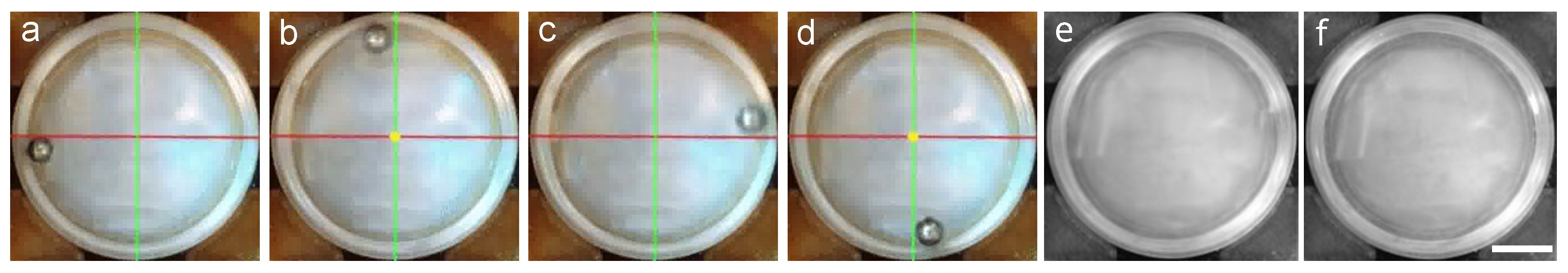
2.3.2. Magnetic Sphere Localization

An object detection module was created for receiving and processing the optical data collected via the camera, including detection of the magnetic sphere across streamed frames. For magnetic sphere localization in each frame, we first obtained a preoperative comparison image (background image), which could then be subtracted from subsequent streamed frames. Following subtraction, images were segmented within the area of interest (Petri dish region of the image) and then filtered to obtain the magnetic sphere’s location. The background image was generated by taking and averaging sequential images of the system with the magnetic sphere positioned at the face of each EM coil via the application of a magnetic field gradient pulling the sphere toward the coil. By actuating each EM sequentially, we positioned the magnetic sphere at the face of each EM coil, collecting an image at each position (Figure 3a–d). We repeated the process, collecting a total of two example images for each of the four magnetic sphere positions. The eight images were then averaged to mitigate the presence of a magnetic sphere, and this averaging step generated a background image that was sufficiently clean to allow for system tracking in future images in which the magnetic sphere could be positioned anywhere in the workspace. Figure (Figure 3e) depicts the generated background image created from the above process of averaging eight images having the magnetic sphere in front of each EM coil. Figure (Figure 3f) presents an image of the Petri dish with the magnetic sphere completely removed from the dish. Our goal with image processing was to accomplish magnetic sphere localization in less than 35 ms, as longer delays in sphere localization result in delays in camera frame acquisition.

2.3.3. Magnetic Sphere Tracking

A user can interactively draw the path for the sphere to follow using the GUI.The system can control the magnetic sphere to follow any trajectory, including those with sharp turns. The system has two customizable parameters for path configuration. The first one is the path interpolation amount, which determines the discretization resolution of the given path. Even if the specified path has only a few anchor points, with a small interpolation amount the path can be finely discretized so that the magnetic sphere can continuously follow a smooth and interpolated path. The second parameter is the path tolerance, which specifies the acceptable distance of the sphere from a path point within which the sphere is considered as successfully following the corresponding path point, and the next target point is then updated. With these two parameters specified by the user, our system ensures locally smooth path specification and sufficient tracking resolution so that any target path can be followed.

2.4. Preprocessing

The collected data were preprocessed before use in model training. Our preprocessing procedure involved first removing all data samples where current scale values were zero. This means that the +X coil input only included values for which the +X coil current was not zero; the same applied for the other coils. Since coils were activated one at a time, the original dataset contained a large proportion of instances in which the current for a given coil was zero, which should be excluded in model training. Following the initial cleaning, approximately 15% of the dataset (≈4500 instances) remained for the training set.

Once data were cleaned of zero values, position data were normalized to a common spatial scale (2D, X–Y plane). Initial x and y positions of the sphere, $X_0$ and $Y_0$, and final positions, $X_f$ and $Y_f$, were all in the range of −17.5 mm and 17.5 mm. The measured distance of the sphere to a coil D was in the range of 5 to 40 mm. Z-score normalization was applied to all data.

2.5. Development of Two Data-Driven Controllers

Two data-driven controllers were independently developed using the same collected data for comparison. The first controller is an ANN-based controller, which learns a predictive model to determine the optimal control signal to move the magnetic particle in the desired direction by the desired travel distance. The second controller is a surface-fitting model, which results in polynomial functions of the distance between the particle and a coil and the desired travel distance. Both models learn the relationship between coil current levels and particle location and travel distance but in different ways. Figure 4 depicts a block diagram of the magnet control system with two controllers. The controllers are detailed in the following sections.

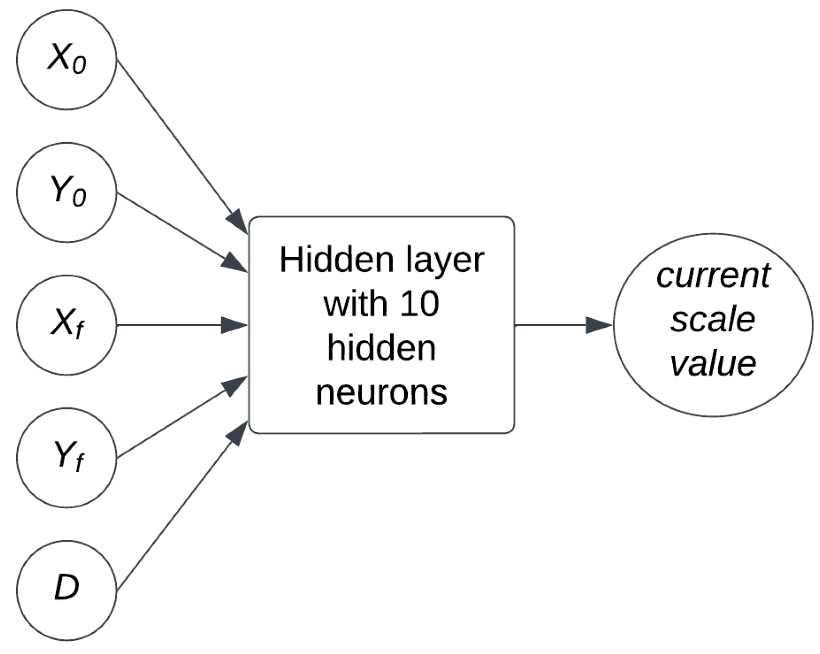
2.5.1. Artificial-Neural-Network-Based Controller

Artificial neural networks were used to control sphere movement in the 2D plane. Four ANNs of the same architecture were trained for the four coils that moved the sphere in the x and y directions (Figure 5). To choose the architecture, the number of hidden layers was varied between 1 and 3, and the number of hidden neurons was tested at 10, 15, 20, 30, and 60 systematically. One hidden layer and ten sigmoid logistic neurons were determined as the best architecture parameters. More complex architectures did not provide any significant increase in performance (measured using the $R^2$ correlation coefficient). Here, we used ANNs based on the generalized regression neural network approach [36]. Each ANN took in five input features, $X_0$, $Y_0$, $X_f$, $Y_f$, and D as defined above. These five inputs were chosen by applying Scikit–Learn’s mutual information regression feature selection method [37] to determine the most relevant features for inclusion. All inputs are expressed in millimeters. Each ANN contained one hidden layer with ten hidden nodes. The output of the ANN was the predicted current scale value of the corresponding coil that would move the sphere to the destination.

Input data were the five measurements collected from tracking the motion of the spherical magnetic sphere as a result of randomly generated pulses applied to the coils. The collected data were split in such a way that $80\%$ was used for training and $20\%$ for testing. Training and testing the ANN models were implemented in the Matlab Deep Learning Toolbox [38] using the Levenberg–Marquardt algorithm [39]. Training the ANN model does not require a specialized computer workstation but can be performeds on any laptop or desktop that has Matlab installed. In our study, training the ANN model took about 10 min only.

2.5.2. Surface Fitting Model-Based Controller

The other control method that we implemented for comparison was the surface fitting model. The same collected data described previously werew used to learn a direct mapping between the applied current scale to a coil and the resultant sphere position. System states such as the viscosity of the liquid agent that the sphere traveled in and hardware setup were also captured by the mapping. A nonlinear regression model was used to represent the mapping, which could then be used to predict the amount of coil current needed to move the sphere in the desired direction by the desired distance. Four models, one for each coil, were implemented by using the ’polyfit’ function in Matlab. Figure 6 illustrates one fitted surface model, which represents the nonlinear association between the sphere distance from a coil and the traveled distance to the current scale.

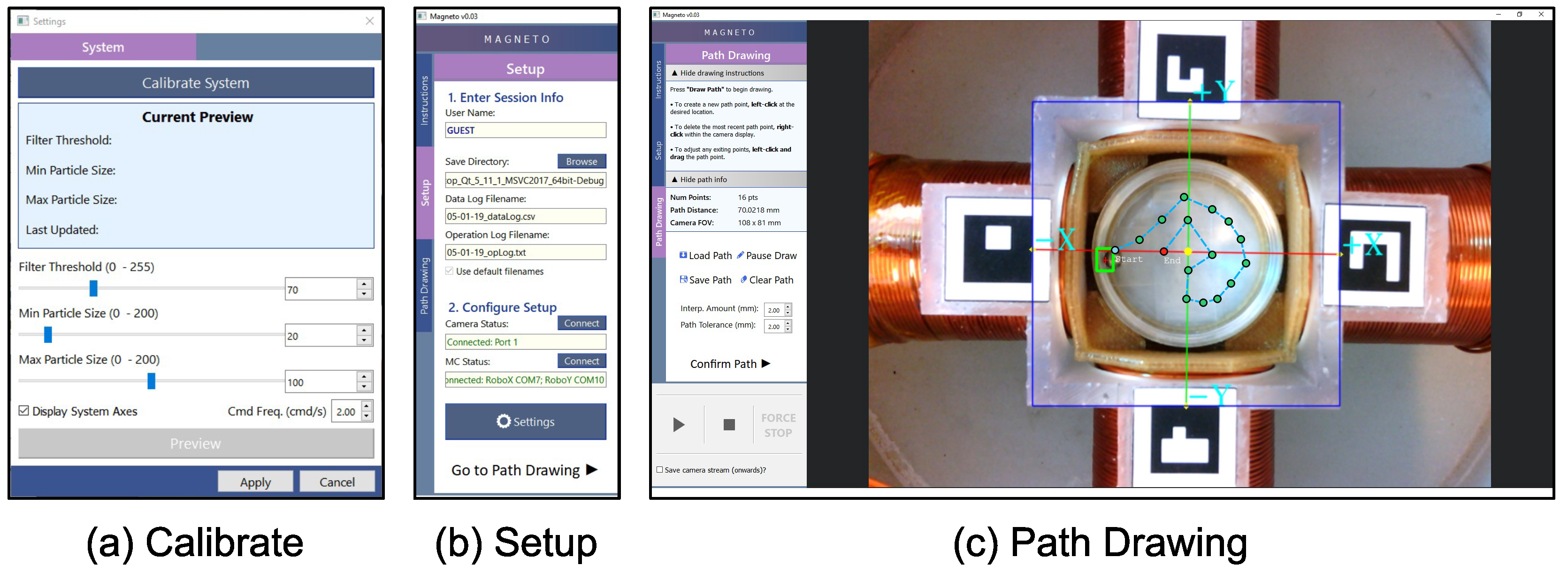
2.6. System Integration and Deployment

Each trained neural network model’s weights and biases were exported to our C++ program so that they could be used with the program controlling the actual system. The C++ matrix library Eigen [40] was used to initialize the weight and bias values for each network. User interaction with the system followed a sequence of steps, starting with system calibration, followed by session setup, after which the user drew a path within the Petri dish area and initiated the controller to move the sphere along the drawn path (Figure 7).

3. Results

3.1. Data Collection

Training data collection included a total of 30,000 instances collected over 3 days. Of the 30,000 instances, approximately 19,000 instances were deemed usable for the training protocol. Unusable instances were characterized by insufficient magnetic sphere motion, unclear visualization of the magnetic sphere, or poor magnetic sphere localization. The configuration of the four coils and the constraint on actuating a single coil at a time made it challenging for the magnetic sphere to move to cover the entire workspace. As such, a majority of the observable instances were constrained to the central and +-shaped central region of the workspace. Figure 8 shows the trajectories of the magnetic sphere over the training period. The majority of the sphere movement was along the horizontal and vertical axes. Much less data were collected in “dead zones”, depicted by regions with a lack of data points (red + signs with green circles).

3.2. Accuracy Comparison of Predicted Current Scales from Two Models

Control current scales predicted by the ANN model and surface fitting models were compared to the applied current scales in the test data. $R^2$ values were calculated to assess the accuracy of the predicted control currents of each model. Figure 9a shows the current scales predicted by the ANN model in comparison to the expected current scales of all the test data instances. The $R^2$ value of the +X coil instances was 0.93 and that of the −X coil was 0.88, both showing the efficacy of the ANN in generating the control currents to move the sphere by the desired distances. In particular, the predicted model showed a close association with the expected current value when they were under a scale factor of 50. Figure 9b shows the current scales predicted by the surface fitting model in comparison to the expected current scales of the test data. The $R^2$ values of the +X and −X coils were 0.65 and 0.73, respectively. A comparison of the $R^2$ values of both horizontal coils showed that the ANN controller performed significantly better than the surface fitting model, with an increase in the $R^2$ values of the current scales of 0.28 and 0.15, respectively, as predicted by the ANN controller.

Table 1. $R^2$ values for each coil based on the surface fitting model and the single-layer, 10-neuron artificial neural network.

Trained Coil	Surface Fitting ${\mathit{R}}^2$	Artificial Neural Network ${\mathit{R}}^2$
+X	0.650	0.932
−X	0.729	0.882
+Y	0.735	0.887
−Y	0.827	0.934
AVERAGE	0.735	0.910

compares the performance of all coils controlled by the ANN model to those controlled by the surface fitting model. The ANN controller outperformed the surface fitting model for all coils, yielding $R^2$ values at least 10% larger than those obtained with the surface fitting model. The averaged ANN model $R^2$ value was 0.91, while that of the surface fitting model was 0.735, demonstrating the significantly better accuracy of the ANN controller.

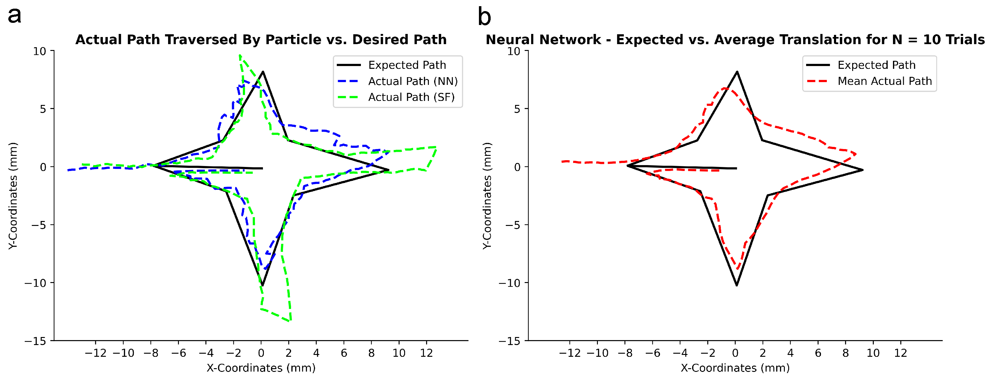
3.3. Comparison of Magnetic Sphere following Trajectories

Both ANN and surface fitting translation models were tested using the same starting sphere location and proposed pathway. Both models allowed translation toward the desired final location following the given path. However, as shown in Figure 10a, the surface fitting model induced frequent and dramatic (several sphere body lengths) overshoot of the sphere position at locations near the coils, especially near the +X and −Y coils. On the other hand, the sphere path that was controlled by the ANN-based controller (shown in blue) was significantly more even throughout the workspace and more closely followed the desired path than the path from the surface fitting model (shown in green). The results suggested that the ANN controller outperformed the surface fitting controller in moving the magnetic sphere. After training, the GMU-Magneto system was capable of controlling the magnetic sphere (4.8 mm diameter NdFeB sphere) with submillimeter precision, using a trained ANN having a single hidden layer with 10 nodes. Across all trials, the average standard deviation from the path for the magnetic sphere was 0.85 mm. The reported results demonstrated the overall bound on the stability of the system. The four actuators were activated one at a time in a sequence. If any single actuator was unreliable, it would have contributed to errors in the overall performance.

4. Discussion

Here, we developed a system that provides a test bed for examining the application of artificial-neural-network-based controllers in object manipulation using electromagnetic fields. Here, we made use of simple and sparse training data in which the overall sampling of the workspace was relatively incomplete. Even though Figure 8 contains a significant amount of the unsampled space, the controller performed well across the entire workspace, as evidenced in Figure 11. A video of the controller moving the magnetic sphere is included as Supplementary Material. ANN controllers were demonstrated to have reasonable (submillimeter) positional resolution in a 2D setting when trained using our simple approach. An additional limitation in the training data set was that the supplied coil current was binary, either 0 A or 20 A. This means that smaller incremental motions of the sphere, as would be expected for coil currents between 0 A and 20 A, were not represented in the training dataset. One future direction is to design a better training process so that the training data incorporate a richer set of positions and trajectories. We anticipate significant improvements in the system with the addition of incremental coil currents. Significantly, the ANN used here contained only one hidden layer, suggesting that fairly simple networks are capable of positional control of simple magnetic objects with accuracy being significantly smaller than the object diameter. More complex workspaces, for example, workspaces having surfaces with varying coefficients of friction, may be ideal testbeds for future experimentation, as computational assessment of varying friction over a workspace is likely challenging to model well.

The system presented here has implications for quickly establishing the ANN-based control of magnet objects via electromagnets. For example, the method we presented for learning control of a spherical magnetic sphere may, in the future, be extended to teach coil arrays to control broad libraries of spheres with diverse magnetic properties. Additionally, the presented method may be applied to highly asymmetric arrays of electromagnets to expedite and simplify expectations of how current supplied to such coils would move a magnetic sphere of a given, and perhaps unknown, magnetic ordering. Additionally, expanding on our approach by applying it to systems of moving electromagnets or permanent magnets may allow for control approaches for complex magnet array systems having numerous variables (magnet position, coil current, magnet angle) to be explored quickly, in a randomized fashion, for the creation of a reliable, low-error control approaches. Future applications of the method may be implemented in other fields using magnetic manipulation, such as microfluidics [41], magnetic drug targeting [42], or the future of microscale devices for medicine [43,44]. Additionally, comparing our ANN approach with control methods based on analytical models may be a future method of benchmarking the ANN results and determining how the ANN may be improved in the future. Combining such control efforts with tracking of more complex and medically relevant devices such as surgical needles [45] and incorporating other nonoptical imaging modalities such as ultrasound (US), computed tomography (CT), or magnetic resonance imaging (MRI) may expand the toolbox of magnetic surgical instrument guidance. However, the overall manipulation of surgical instruments requires significant on-the-fly tunability, and control paradigms that can begin to address the dynamics of in vivo operation are only just now emerging [46,47].

4.1. Magnetic Sphere Detection Sensitivity Analysis

To assess system tolerance to various lighting conditions, we recorded the sphere location under three different lighting scenarios: dark room of ≈6 lux (Figure 12a), ambient overhead room lighting of ≈80 lux (Figure 12b), and direct overhead lighting supplied by a lamp of ≈220 lux (Figure 12c). For each determination, a video of the sphere was collected for 60 s, during which time the sphere was not manipulated. During the 60 s video under each lighting condition, 50 frames were collected and segmented to estimate sphere location. The standard deviation in sphere location for each lighting condition was computed. Dark room, ambient, and direct overhead lamp lighting conditions yielded standard deviations in sphere position of 0.34 mm, 0.05 mm, and 0.13 mm, respectively. We suspect that the ambient lighting condition yielded the lower standard deviation in sphere position because the dark room condition provided insufficient illuminance to reliably determine the edges of the sphere, and the direct overhead lamp condition yielded saturated pixels and shadows that also inhibited accurate edge detection in our object detection scheme.

4.2. GUI Response Time

For the GUI to be practical, reasonable response times are required for a seamless user interface. We quantified system response times to ensure smooth operation, as shown in

Table 2. Typical lag time values for significant GUI functions.

Function	Average Lag Time (ms)	Standard Deviation (ms)
Startup	1287.13	16.59
Camera Connection	987.38	182.76
Motor Controller Connection	10.81	0.59
Open Settings Window	52.38	2.11
Apply Settings Window Edits	0.16	0.10
Start/Pause System Operation	1.98	0.56
Stop Hardware Execution	0.09	0.08

. Specifically, we assessed the GUI functions of the startup, camera connection, motor controller connection, opening the settings window, applying settings window edits, starting/pausing system operation, and stopping hardware execution. We found that startup and camera connection initiated long delays, with each operation taking ≈1 s. Beyond those two functions, all other functions were completed in significantly less than 100 ms.

Future work demonstrating operability in an array of light sources, and possibly under actively changing lighting conditions, may shed light on how the anticipation of dynamic lighting conditions could be incorporated into the training set for untethered magnetic manipulation systems. Various laboratories have applied advanced learning techniques such as reinforcement learning to the problem of controlling small magnetic devices [48,49,50], and we acknowledge that the application of such learning approaches would improve the performance of our controller. However, here, we emphasize the ability to control a simple magnetic sphere using very simple regression models and a small sample data set. Additionally, future efforts may include incorporating finite element model simulations for the controller and coil array. Finally, the proposed ANN model can be improved by adding the desired travel time as another input to provide transient movement control in addition to the current position control.

5. Conclusions and Future Work

We developed a simple, easy-to-implement AI-based controller for an electromagnetic system, tested its performance in a four-coil system, and compared it to a surface fitting controller. We described the electromagnet system, magnetic sphere tracking method, our approach for data collection, and ANN structure. We then quantified the ANN’s performance in comparison to that of a surface fitting control approach. Our results showed that a simple one-layer artificial neural network could be conveniently trained to control the magnetic sphere’s position to follow desired trajectories. The significance of the method presented lies in its simplicity, in that no prior physics knowledge is used in the ANN, and the collected data rely on the actuation of a single coil at a time, with only a single current value used in the data collection. No assumption needs to be made on the system configuration or characteristics, as the ANN model was able to learn them through the training data. Naturally, more complex exploration of the parameter space, such as activating multiple coils at a time or activating coils with incremental current values (i.e., currents between 1 A and 20 A) would significantly expand the original data set and improve the accuracy and precision of the ANN-based controller.

References

1. Martin, J.W.; Scaglioni, B.; Norton, J.C.; Subramanian, V.; Arezzo, A.; Obstein, K.L.; Valdastri, P. Enabling the future of colonoscopy with intelligent and autonomous magnetic manipulation. Nat. Mach. Intell. 2020, 2, 595–606. [Google Scholar] [CrossRef] [PubMed]
2. Kumar, P.; Malik, S.; Toyserkani, E.; Khamesee, M.B. Development of an electromagnetic micromanipulator levitation system for metal additive manufacturing applications. Micromachines 2022, 13, 585. [Google Scholar] [CrossRef] [PubMed]
3. Cao, Q.; Fan, Q.; Chen, Q.; Liu, C.; Han, X.; Li, L. Recent advances in manipulation of micro-and nano-objects with magnetic fields at small scales. Mater. Horizons 2020, 7, 638–666. [Google Scholar] [CrossRef]
4. Yang, Z.; Zhang, L. Magnetic actuation systems for miniature robots: A review. Adv. Intell. Syst. 2020, 2, 2000082. [Google Scholar] [CrossRef]
5. Chen, X.Z.; Jang, B.; Ahmed, D.; Hu, C.; De Marco, C.; Hoop, M.; Mushtaq, F.; Nelson, B.J.; Pané, S. Small-scale machines driven by external power sources. Adv. Mater. 2018, 30, 1705061. [Google Scholar] [CrossRef] [PubMed]
6. Sitti, M.; Ceylan, H.; Hu, W.; Giltinan, J.; Turan, M.; Yim, S.; Diller, E. Biomedical applications of untethered mobile milli/microrobots. Proc. IEEE 2015, 103, 205–224. [Google Scholar] [CrossRef] [PubMed]
7. Xu, T.; Yu, J.; Yan, X.; Choi, H.; Zhang, L. Magnetic actuation based motion control for microrobots: An overview. Micromachines 2015, 6, 1346–1364. [Google Scholar] [CrossRef]
8. Yang, L.; Zhang, L. Motion control in magnetic microrobotics: From individual and multiple robots to swarms. Annu. Rev. Control Robot. Auton. Syst. 2021, 4, 509–534. [Google Scholar] [CrossRef]
9. Abbott, J.J.; Diller, E.; Petruska, A.J. Magnetic methods in robotics. Annu. Rev. Control Robot. Auton. Syst. 2020, 3, 57–90. [Google Scholar] [CrossRef]
10. Komaee, A.; Shapiro, B. Steering a ferromagnetic particle by optimal magnetic feedback control. IEEE Trans. Control Syst. Technol. 2011, 20, 1011–1024. [Google Scholar] [CrossRef]
11. Komaee, A. Feedback control for transportation of magnetic fluids with minimal dispersion: A first step toward targeted magnetic drug delivery. IEEE Trans. Control Syst. Technol. 2016, 25, 129–144. [Google Scholar] [CrossRef]
12. Fang, W.Z.; Xiong, T.; Pak, O.S.; Zhu, L. Data-driven intelligent manipulation of particles in microfluidics. Adv. Sci. 2023, 10, 2205382. [Google Scholar] [CrossRef]
13. Chapin, S.C.; Germain, V.; Dufresne, E.R. Automated trapping, assembly, and sorting with holographic optical tweezers. Opt. Express 2006, 14, 13095–13100. [Google Scholar] [CrossRef] [PubMed]
14. Cohen, A.E. Control of nanoparticles with arbitrary two-dimensional force fields. Phys. Rev. Lett. 2005, 94, 118102. [Google Scholar] [CrossRef]
15. Zhou, Q.; Sariola, V.; Latifi, K.; Liimatainen, V. Controlling the motion of multiple objects on a Chladni plate. Nat. Commun. 2016, 7, 12764. [Google Scholar] [CrossRef] [PubMed]
16. Probst, R.; Lin, J.; Komaee, A.; Nacev, A.; Cummins, Z.; Shapiro, B. Planar steering of a single ferrofluid drop by optimal minimum power dynamic feedback control of four electromagnets at a distance. J. Magn. Magn. Mater. 2011, 323, 885–896. [Google Scholar] [CrossRef] [PubMed]
17. Ongaro, F.; Pane, S.; Scheggi, S.; Misra, S. Design of an electromagnetic setup for independent three-dimensional control of pairs of identical and nonidentical microrobots. IEEE Trans. Robot. 2018, 35, 174–183. [Google Scholar] [CrossRef]
18. Liu, Y.; Feng, Y.; An, M.; Sarwar, M.T.; Yang, H. Advances in Finite Element Analysis of External Field-Driven Micro/Nanorobots: A Review. Adv. Intell. Syst. 2023, 5, 2200466. [Google Scholar] [CrossRef]
19. Weerasooriya, S.; El-Sharkawi, M.A. Identification and control of a dc motor using back-propagation neural networks. IEEE Trans. Energy Convers. 1991, 6, 663–669. [Google Scholar] [CrossRef]
20. Kolo, B.A. Neural Networks in Magnetic Guidance; University of Virginia: Charlottesville, VA, USA, 1998. [Google Scholar]
21. Yu, R.; Charreyron, S.L.; Boehler, Q.; Weibel, C.; Chautems, C.; Poon, C.C.; Nelson, B.J. Modeling electromagnetic navigation systems for medical applications using random forests and artificial neural networks. In Proceedings of the 2020 IEEE International Conference on Robotics and Automation (ICRA), Paris, France, 31 May–31 August 2020; IEEE: Piscataway, NJ, USA, 2020; pp. 9251–9256. [Google Scholar]
22. Kazemzadeh Heris, P.; Khamesee, M.B. Design and fabrication of a magnetic actuator for torque and force control estimated by the ann/sa algorithm. Micromachines 2022, 13, 327. [Google Scholar] [CrossRef]
23. Tariverdi, A.; Venkiteswaran, V.K.; Richter, M.; Elle, O.J.; Tørresen, J.; Mathiassen, K.; Misra, S.; Martinsen, Ø.G. A recurrent neural-network-based real-time dynamic model for soft continuum manipulators. Front. Robot. AI 2021, 8, 631303. [Google Scholar] [CrossRef]
24. Liu, J.; Wu, X.; Huang, C.; Manamanchaiyaporn, L.; Shang, W.; Yan, X.; Xu, T. 3-D autonomous manipulation system of helical microswimmers with online compensation update. IEEE Trans. Autom. Sci. Eng. 2020, 18, 1380–1391. [Google Scholar] [CrossRef]
25. Behrens, M.R.; Ruder, W.C. Smart Magnetic Microrobots Learn to Swim with Deep Reinforcement Learning. Adv. Intell. Syst. 2022, 4, 2200023. [Google Scholar] [CrossRef]
26. Salehi, M.; Nejat Pishkenari, H.; Zohoor, H. Position control of a wheel-based miniature magnetic robot using neuro-fuzzy network. Robotica 2022, 40, 3895–3910. [Google Scholar] [CrossRef]
27. Turan, M.; Ornek, E.P.; Ibrahimli, N.; Giracoglu, C.; Almalioglu, Y.; Yanik, M.F.; Sitti, M. Unsupervised odometry and depth learning for endoscopic capsule robots. In Proceedings of the 2018 IEEE/RSJ International Conference on Intelligent Robots and Systems (IROS), Madrid, Spain, 1–5 October 2018; IEEE: Piscataway, NJ, USA, 2018; pp. 1801–1807. [Google Scholar]
28. Norton, J.C.; Slawinski, P.R.; Lay, H.S.; Martin, J.W.; Cox, B.F.; Cummins, G.; Desmulliez, M.P.; Clutton, R.E.; Obstein, K.L.; Cochran, S.; et al. Intelligent magnetic manipulation for gastrointestinal ultrasound. Sci. Robot. 2019, 4, eaav7725. [Google Scholar] [CrossRef] [PubMed]
29. Ahmad, O.F.; Mori, Y.; Misawa, M.; Kudo, S.E.; Anderson, J.T.; Bernal, J.; Berzin, T.M.; Bisschops, R.; Byrne, M.F.; Chen, P.J.; et al. Establishing key research questions for the implementation of artificial intelligence in colonoscopy: A modified Delphi method. Endoscopy 2021, 53, 893–901. [Google Scholar] [CrossRef] [PubMed]
30. Fan, Q.; Zhang, P.; Qu, J.; Huang, W.; Liu, X.; Xie, L. Dynamic magnetic field generation with high accuracy modeling applied to magnetic robots. IEEE Trans. Magn. 2021, 57, 1–10. [Google Scholar] [CrossRef]
31. Barnoy, Y.; Erin, O.; Raval, S.; Pryor, W.; Mair, L.O.; Weinberg, I.N.; Diaz-Mercado, Y.; Krieger, A.; Hager, G.D. Control of Magnetic Surgical Robots With Model-Based Simulators and Reinforcement Learning. IEEE Trans. Med. Robot. Bionics 2022, 4, 945–956. [Google Scholar] [CrossRef]
32. Liu, D. The Application of Machine Learning for Designing and Controlling Electromagnetic Fields. Ph.D. Thesis, University of Wisconsin–Madison, Madison, WI, USA, 2021. [Google Scholar]
33. Huang, Z.; Zhu, J.; Shao, J.; Wei, Z.; Tang, J. Recurrent neural network based high-precision position compensation control of magnetic levitation system. Sci. Rep. 2022, 12, 11435. [Google Scholar] [CrossRef]
34. Charreyron, S.L.; Boehler, Q.; Kim, B.; Weibel, C.; Chautems, C.; Nelson, B.J. Modeling electromagnetic navigation systems. IEEE Trans. Robot. 2021, 37, 1009–1021. [Google Scholar] [CrossRef]
35. Garrido-Jurado, S.; Muñoz-Salinas, R.; Madrid-Cuevas, F.J.; Marín-Jiménez, M.J. Automatic generation and detection of highly reliable fiducial markers under occlusion. Pattern Recognit. 2014, 47, 2280–2292. [Google Scholar] [CrossRef]
36. Specht, D.F. A general regression neural network. IEEE Trans. Neural Netw. 1991, 2, 568–576. [Google Scholar] [CrossRef]
37. Pedregosa, F.; Varoquaux, G.; Gramfort, A.; Michel, V.; Thirion, B.; Grisel, O.; Blondel, M.; Prettenhofer, P.; Weiss, R.; Dubourg, V.; et al. Scikit-learn: Machine Learning in Python. J. Mach. Learn. Res. 2011, 12, 2825–2830. [Google Scholar]
38. Deep Learning Toolbox, Version: 9.4 (R2022b); The MathWorks Inc.: Natick, MA, USA, 2022.
39. Moré, J.J. The Levenberg-Marquardt algorithm: Implementation and theory. In Numerical Analysis, Proceedings of the Biennial Conference, Dundee, UK, June 28–July 1 1977; Springer: Berlin/Heidelberg, Germany, 2006; pp. 105–116. [Google Scholar]
40. Guennebaud, G.; Jacob, B.; Avery, P.; Bachrach, A.; Barthelemy, S.; Becker, C.; Benjamin, D.; Berger, C.; Berres, A.; Blanco, J.L.; et al. Eigen v3. 2010. Available online: http://eigen.tuxfamily.org (accessed on 15 January 2019).
41. Galan, E.A.; Zhao, H.; Wang, X.; Dai, Q.; Huck, W.T.; Ma, S. Intelligent microfluidics: The convergence of machine learning and microfluidics in materials science and biomedicine. Matter 2020, 3, 1893–1922. [Google Scholar] [CrossRef]
42. Shapiro, B.; Kulkarni, S.; Nacev, A.; Muro, S.; Stepanov, P.Y.; Weinberg, I.N. Open challenges in magnetic drug targeting. Wiley Interdiscip. Rev. Nanomed. Nanobiotechnol. 2015, 7, 446–457. [Google Scholar] [CrossRef] [PubMed]
43. Vitol, E.A.; Novosad, V.; Rozhkova, E.A. Microfabricated magnetic structures for future medicine: From sensors to cell actuators. Nanomedicine 2012, 7, 1611–1624. [Google Scholar] [CrossRef] [PubMed]
44. Shao, Y.; Fahmy, A.; Li, M.; Li, C.; Zhao, W.; Sienz, J. Study on magnetic control systems of micro-robots. Front. Neurosci. 2021, 15, 736730. [Google Scholar] [CrossRef] [PubMed]
45. Hong, A.; Petruska, A.J.; Zemmar, A.; Nelson, B.J. Magnetic control of a flexible needle in neurosurgery. IEEE Trans. Biomed. Eng. 2020, 68, 616–627. [Google Scholar] [CrossRef]
46. Kinross, J.M.; Mason, S.E.; Mylonas, G.; Darzi, A. Next-generation robotics in gastrointestinal surgery. Nat. Rev. Gastroenterol. Hepatol. 2020, 17, 430–440. [Google Scholar] [CrossRef] [PubMed]
47. Connor, M.J.; Dasgupta, P.; Ahmed, H.U.; Raza, A. Autonomous surgery in the era of robotic urology: Friend or foe of the future surgeon? Nat. Rev. Urol. 2020, 17, 643–649. [Google Scholar] [CrossRef] [PubMed]
48. Brablc, M.; Žegklitz, J.; Grepl, R.; Babuška, R. Control of Magnetic Manipulator Using Reinforcement Learning Based on Incrementally Adapted Local Linear Models. Complexity 2021, 2021, 6617309. [Google Scholar] [CrossRef]
49. Abbasi, S.A.; Ahmed, A.; Noh, S.; Gharamaleki, N.L.; Kim, S.; Chowdhury, A.M.B.; Kim, J.y.; Pané, S.; Nelson, B.J.; Choi, H. Autonomous 3D positional control of a magnetic microrobot using reinforcement learning. Nat. Mach. Intell. 2024, 6, 92–105. [Google Scholar] [CrossRef]
50. Cai, M.; Wang, Q.; Qi, Z.; Jin, D.; Wu, X.; Xu, T.; Zhang, L. Deep Reinforcement Learning Framework-Based Flow Rate Rejection Control of Soft Magnetic Miniature Robots. IEEE Trans. Cybern. 2022, 53, 7699–7711. [Google Scholar] [CrossRef] [PubMed]
Figure 1. (a) Schematic diagram of the experimental setup. (b) Picture of the actual setup mounted on a 3D-printed base with labeled dimensions. ArUco markers were assigned to each of the four coils. Centered in the coil array sits a Petri dish (35 mm diameter).
Robotics 13 00039 g001
Figure 2. Data collection procedure flowchart.
Robotics 13 00039 g002
Figure 3. Background image generated by image averaging works well. (ad) Images of a magnetic sphere positioned in front of EM coils. (e) Background image created by averaging (ad). (f) Background image was taken with the magnetic sphere removed from the Petri dish. The scale bar is 1 cm.
Robotics 13 00039 g003
Figure 4. Block diagram of the magnet control system.
Robotics 13 00039 g004
Figure 5. Four ANNs of the same architecture were trained to compute the current scale values of the four coils. X 0 , Y 0 : initial x and y positions of the sphere, respectively; X f and Y f : final x and y positions of the sphere, respectively; D: measured distance of the sphere to a coil.
Robotics 13 00039 g005
Figure 6. An example of the learned surface model, which maps the sphere distance to the corresponding coil and the traveled distance of the sphere to the current scale applied.
Robotics 13 00039 g006
Figure 7. GUI allows the user to first (a) calibrate the system, choosing filter thresholds, and minimum and maximum particle sizes (pixels). (b) Setup and user–directed file naming, camera status, and motor controller status. (c) How a user interacts with the system. First, the start location, end location, and waypoints are selected, and system control is initiated.
Robotics 13 00039 g007
Figure 8. Training data were collected continuously by tracking magnetic sphere positions after the application of a sequence of randomly distributed magnetic pulses. Pulse protocol as described above.
Robotics 13 00039 g008
Figure 9. Performance comparison of current scale factor inference between the ANN +X and −X coil models (a) and the surface-fitting +X and −X coil models (b).
Robotics 13 00039 g009
Figure 10. Path traversal comparison. Desired and actual paths traversed by the particle using the two different motion models (a). The average path traversed by the particle across N = 10 trials using the neural network model (b).
Robotics 13 00039 g010
Figure 11. Sphere manipulation demonstration. Using a GUI, a user-defined pattern is proposed having a start position (a), 10 intermediate waypoints (bk), and a finish position (l). Despite the overwhelming data on sphere response to the random distribution of pulses being centered on the cardinal axes of the workspace (Figure 8), the system readily moves the magnetic sphere through a broad range of the workspace (traversing 270° around the center point, (aj)) and finally returns the magnetic sphere to the center of the workspace (k,l).
Robotics 13 00039 g011
Figure 12. Comparison of sphere location detection in various laboratory lighting scenarios. (a) Dark room with only sunlight, approximately 6 lux. (b) Ambient lighting from room lights, approximately 80 lux. (c) Direct lighting from lamp positioned over Petri dish and coil array, approximately 220 lux.
Robotics 13 00039 g012