

How Does the 2D/3D Urban Morphology Affect the Urban Heat Island across Urban Functional Zones? A Case Study of Beijing, China
Abstract
1. Introduction
2. Study Area and Dataset
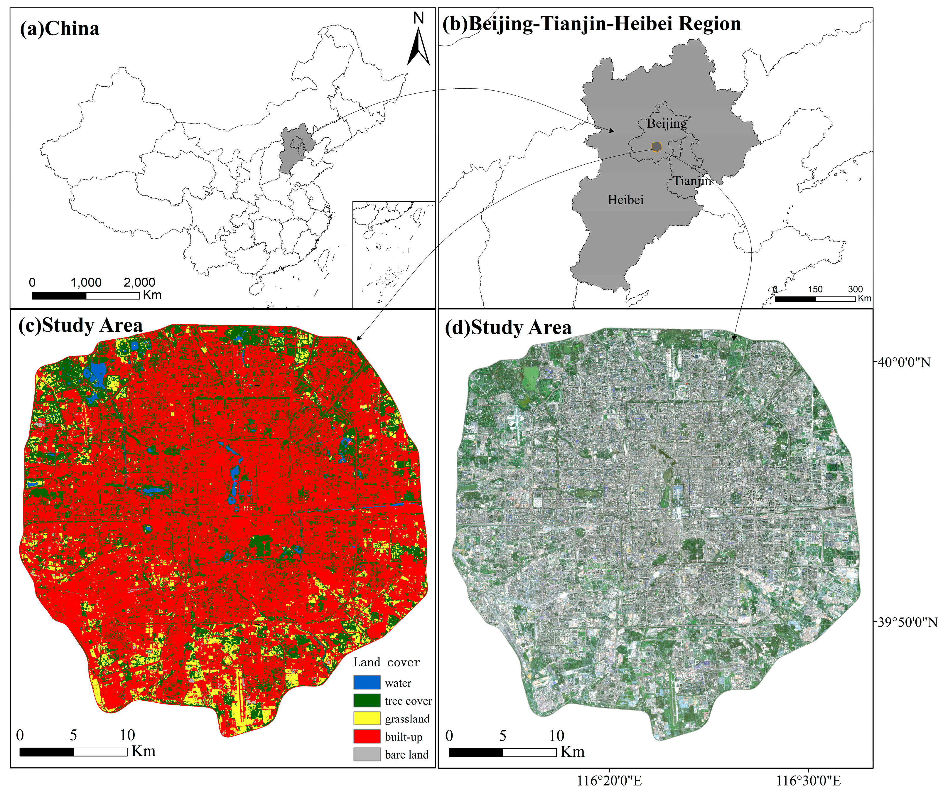
2.1. Study Area
2.2. Dataset
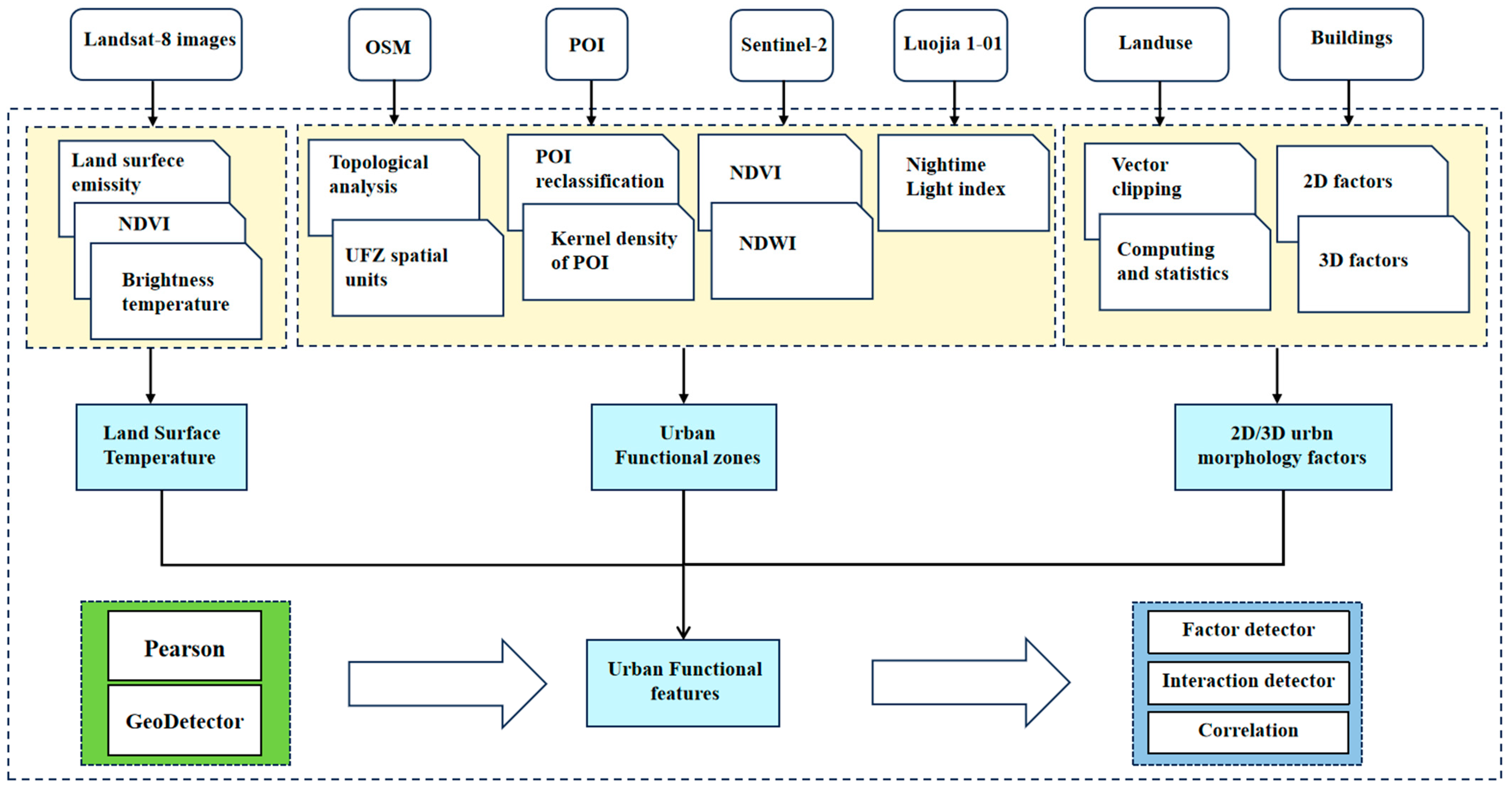
3. Method
3.1. LST Inversion
3.2. UFZ Mapping
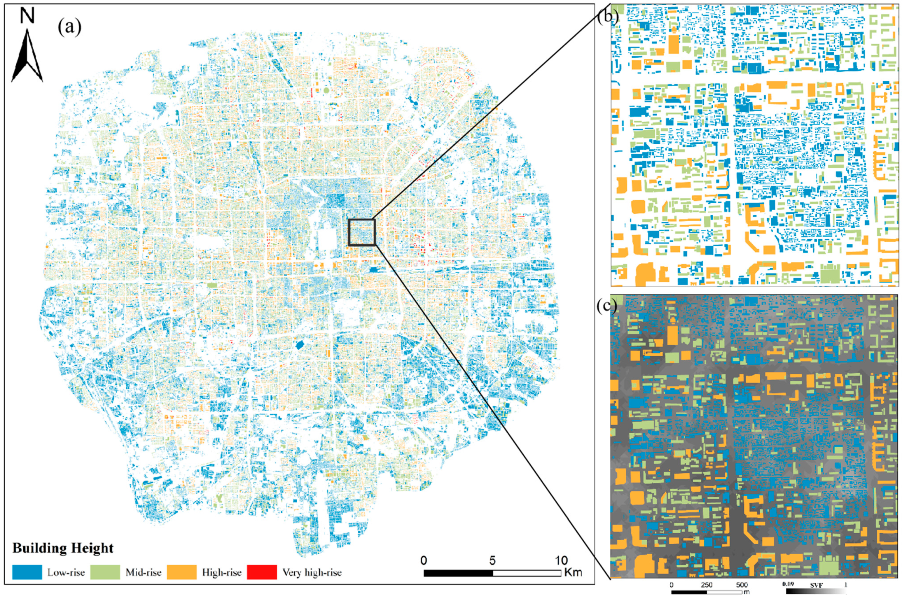
3.3. 2D/3D Urban Morphology Factors
3.4. Data Analysis Methods
3.4.1. Pearson Correlation Analysis
3.4.2. GeoDetector
4. Results
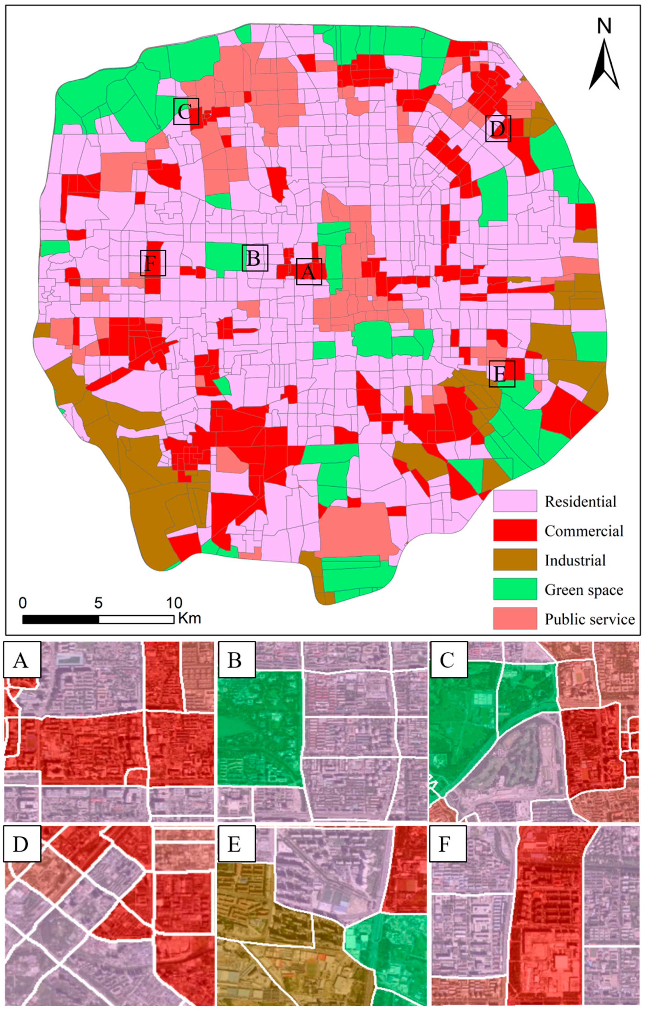
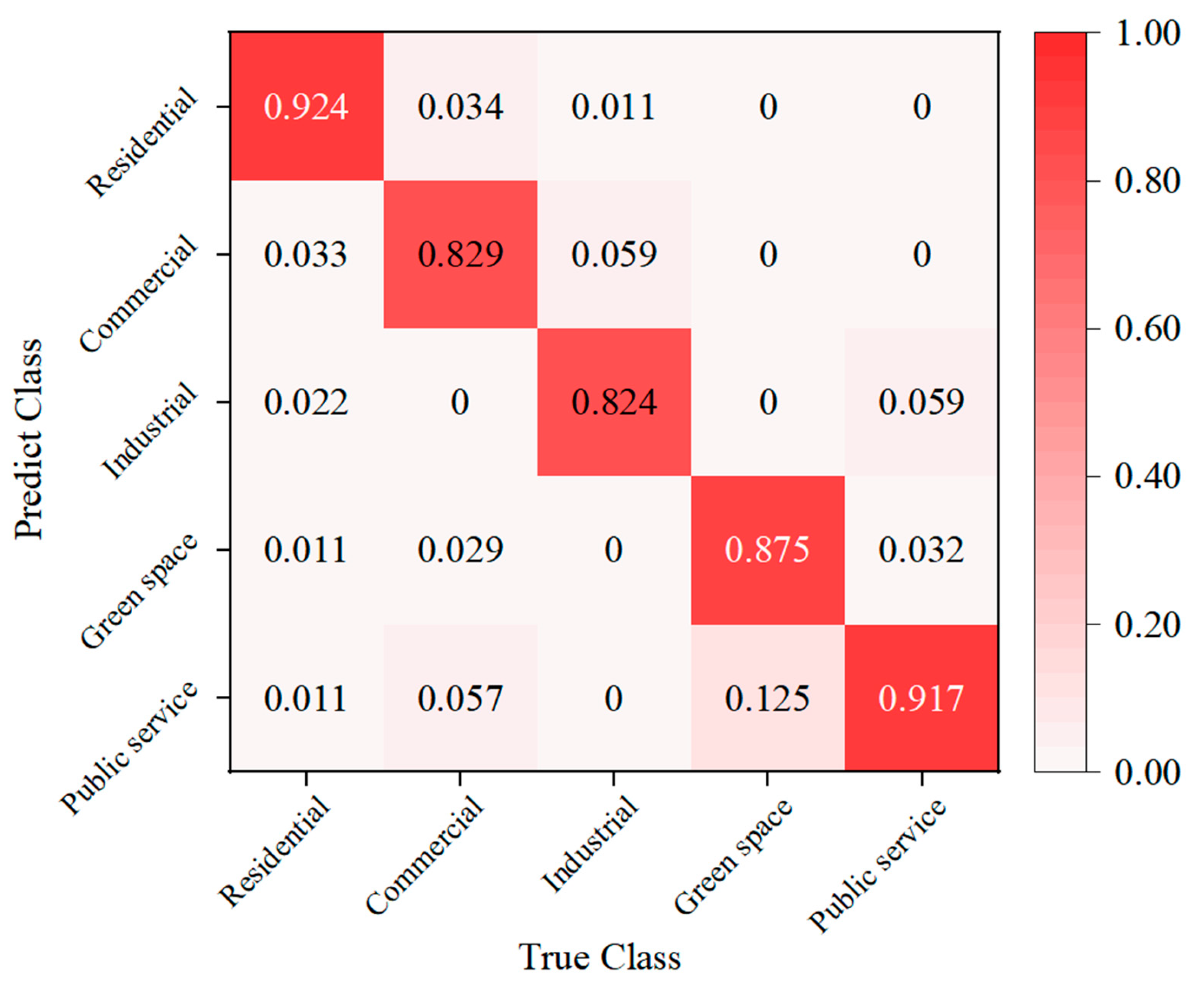
4.1. Results of UFZ Mapping
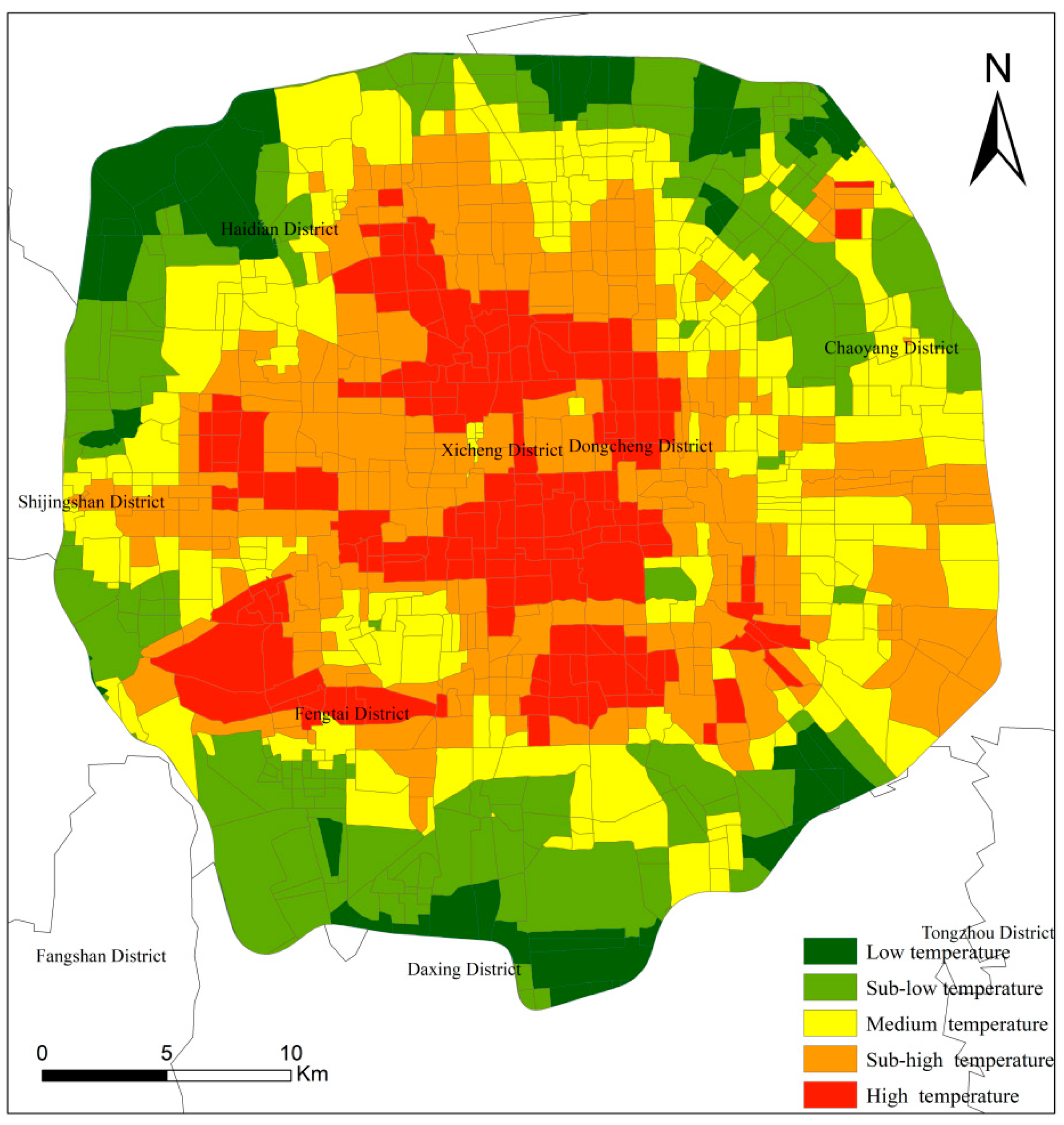
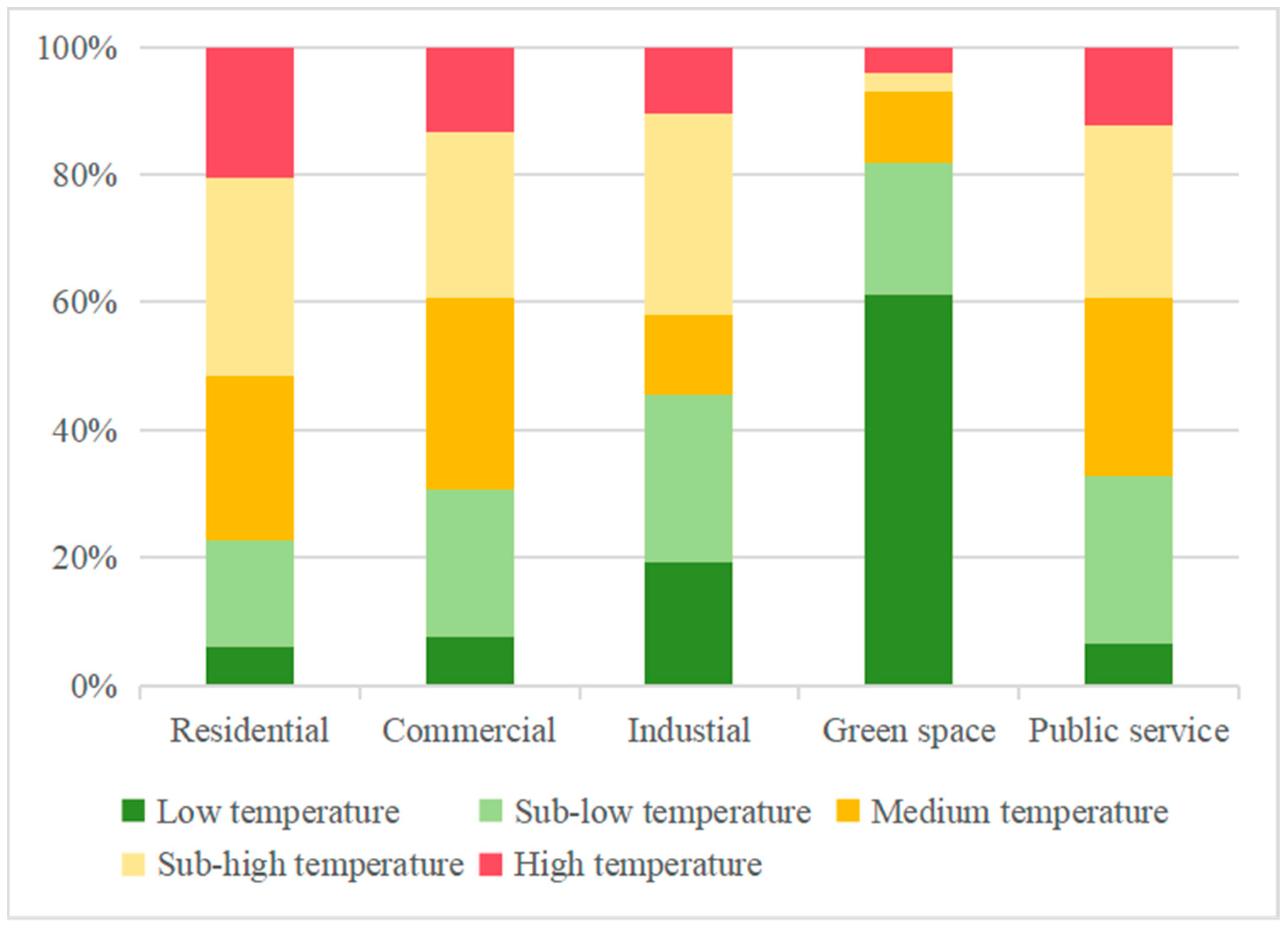
4.2. LST Inversion Results
4.3. Factors Influencing Analysis
4.3.1. Correlation between 2D/3D Factors and LST
4.3.2. The Influence of 2D/3D Factors on LST
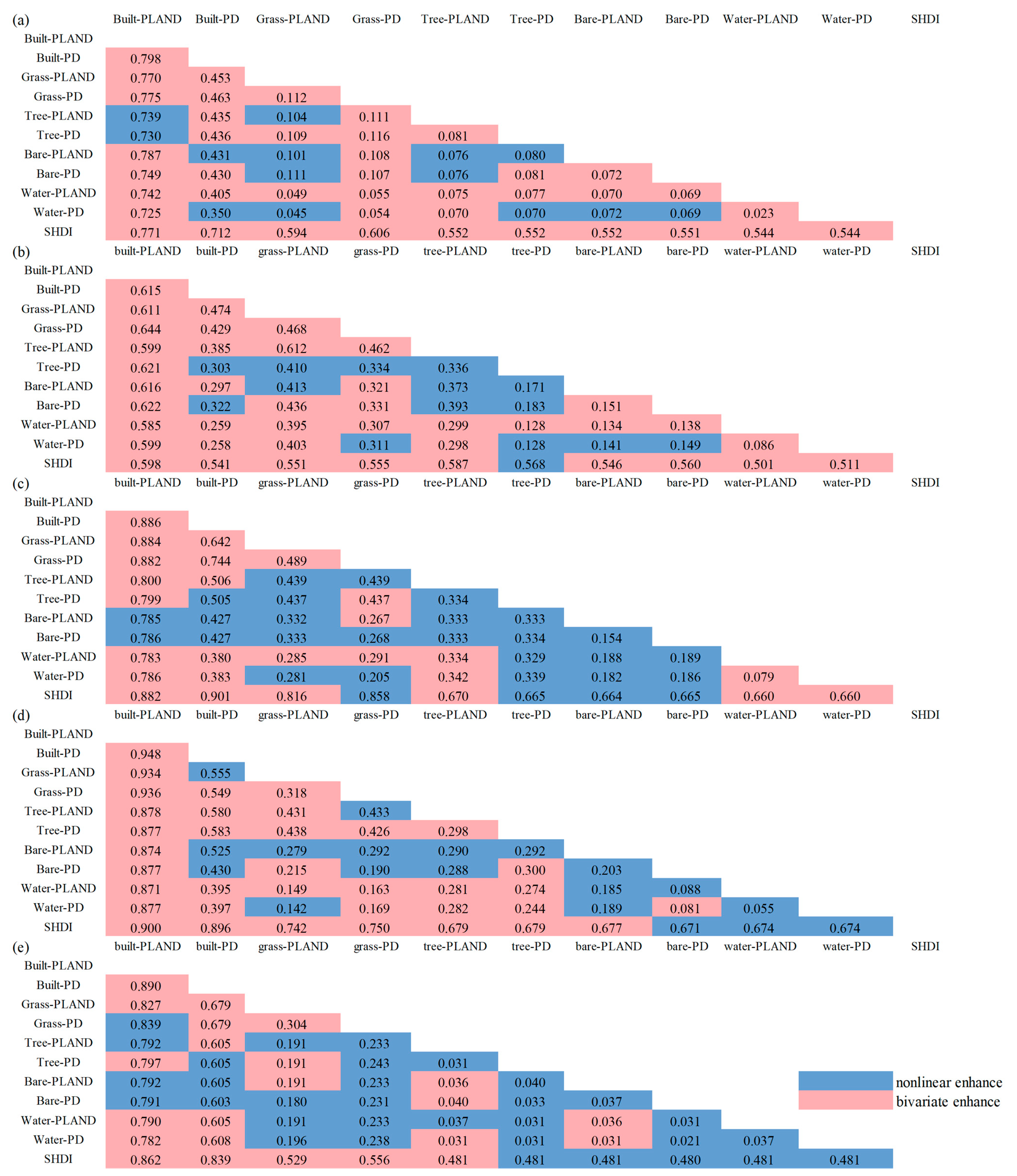
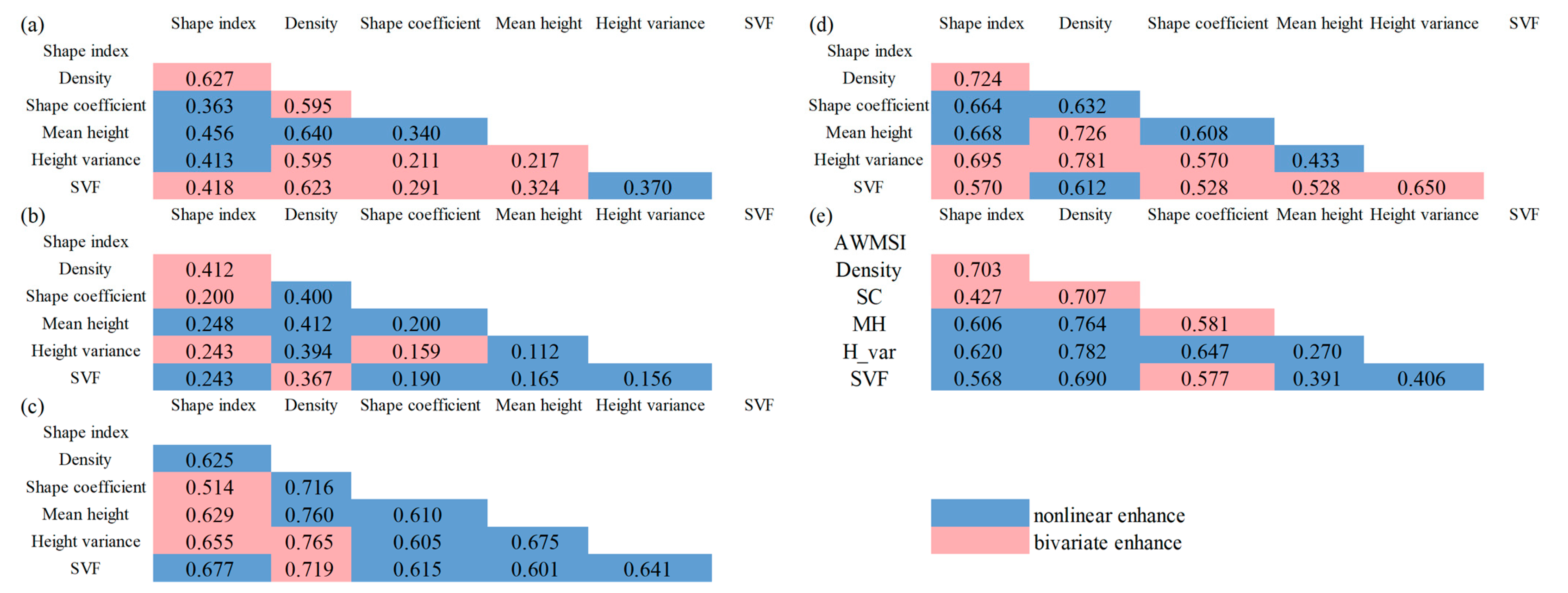
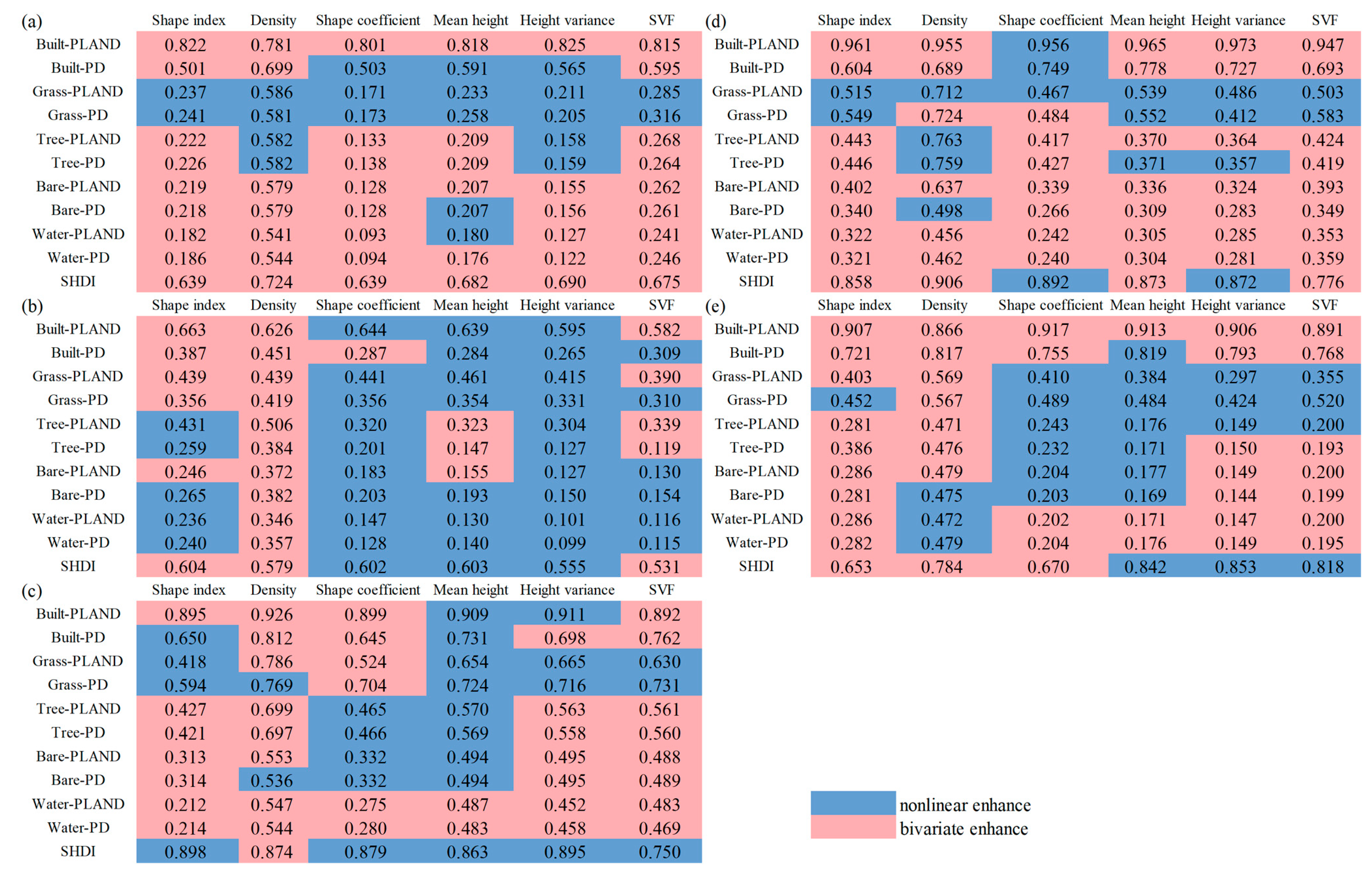
4.3.3. Factor Interaction Analysis
5. Discussion
5.1. Impact of 2D/3D Urban Morphology on LST
5.2. Comparison with Other Studies
5.3. Limitations
5.4. Urban Planning Recommendations
6. Conclusions
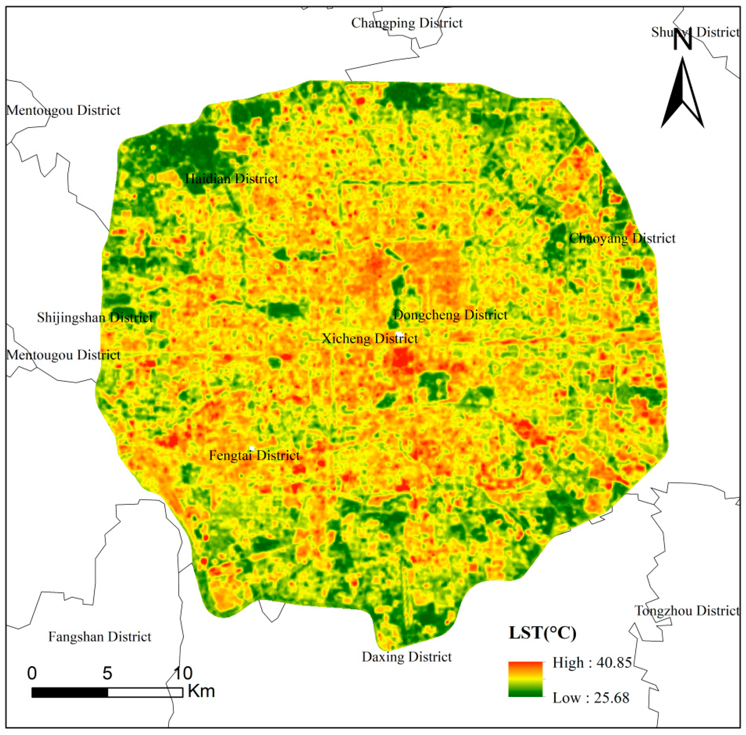
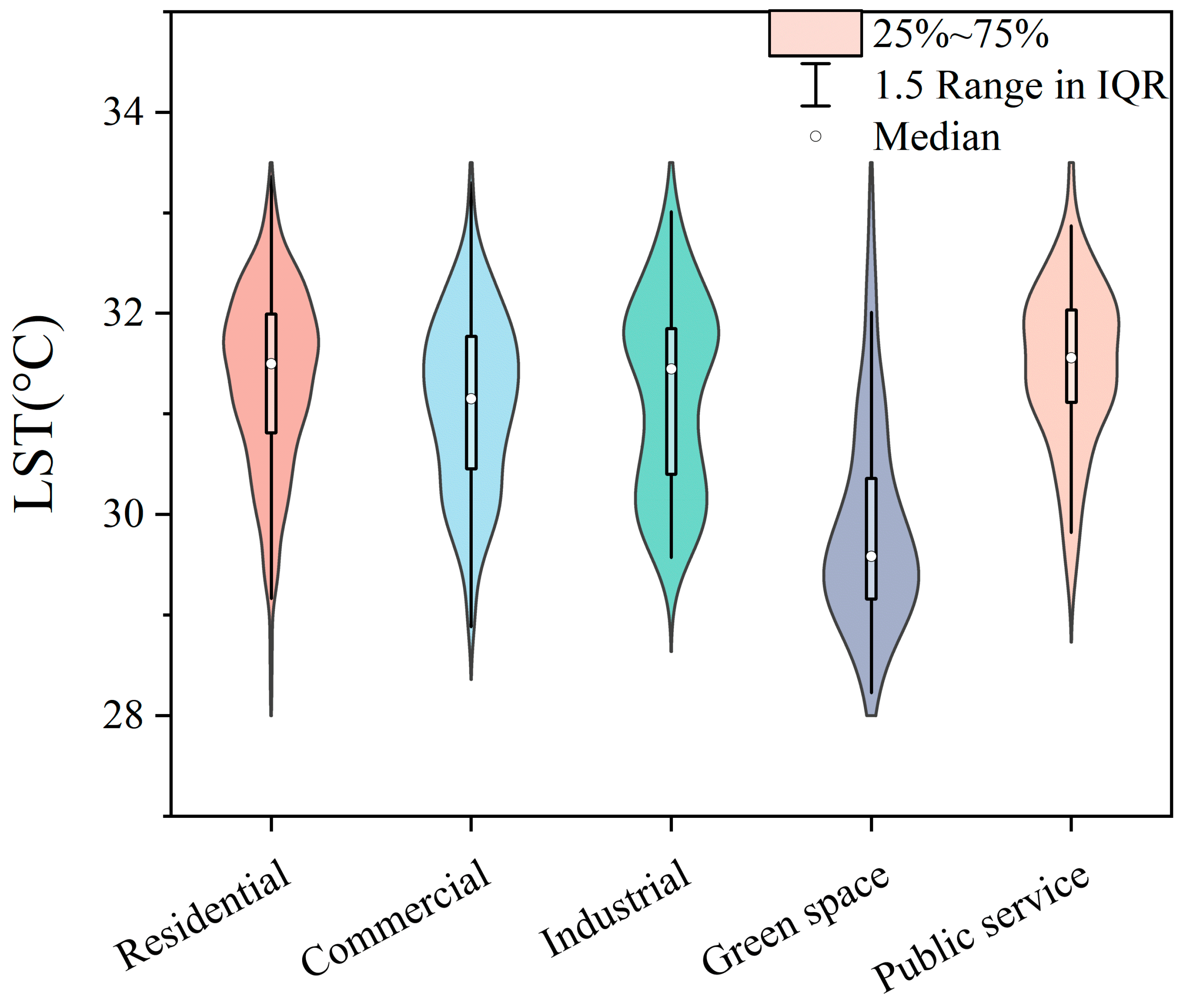
- The LST in Beijing within the Fifth Ring Road exhibits an overall pattern of “higher in the center, lower in the periphery”. Residential zones have the highest LST, followed by industrial zones. Notably, the public service zones show the highest standard deviation (0.95 °C), while the residential zones have the lowest (0.87 °C).
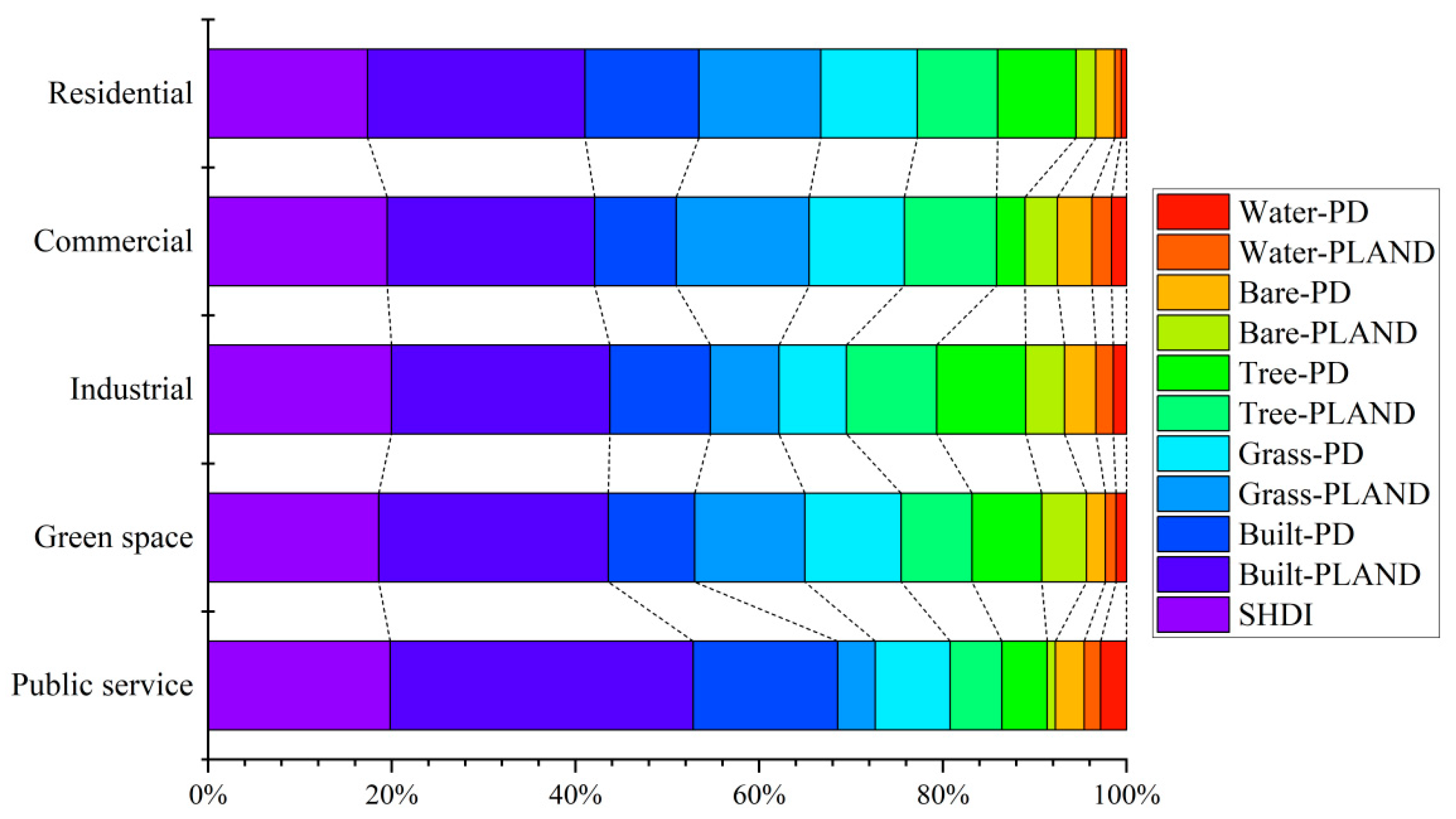
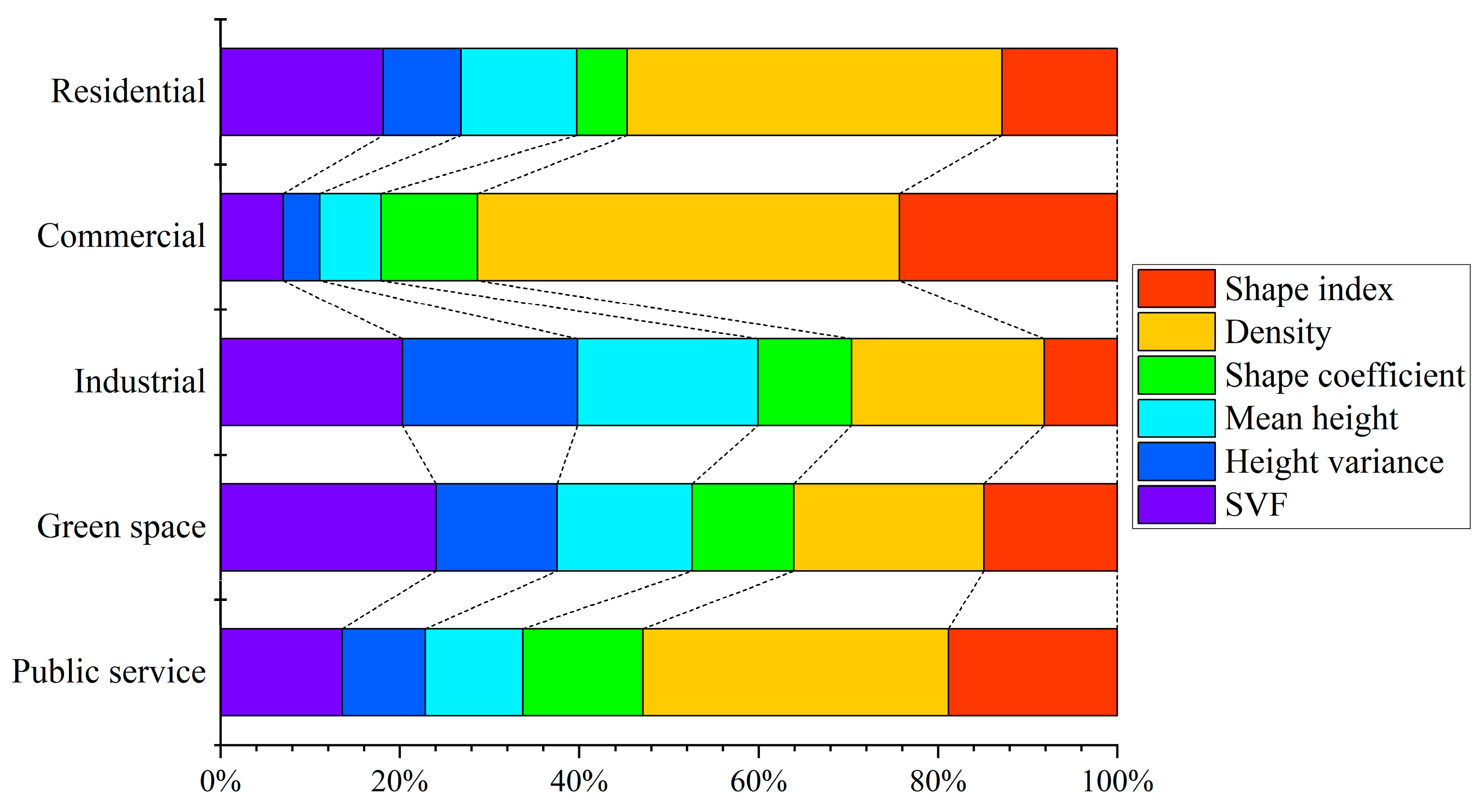
- Significant correlations exist between LST and both 2D and 3D urban morphology parameters. GeoDetector results indicate that built-PLAND and SHDI are the primary factors influencing LST in 2D urban morphology, while density, SVF, and shape index play a major role in 3D urban morphology. Three-dimensional urban morphology, including density, SVF, and shape index, also influences the variation of LST. Daytime LST tends to increase with building density, becoming higher as the complexity of building shapes increases. The SVF regulates ventilation, incoming solar radiation, and captures thermal radiation simultaneously, affecting LST. Therefore, it is advisable to reduce building density, increase building height, simplify building shapes, and disperse buildings. Additionally, the spatial distribution of trees, grasslands, and water bodies also helps mitigate LST, suggesting the adoption of fragmented distributions.
- In interaction detection results, all UFZs exhibit the highest interaction with the built-PLAND factor, with q-values as follows: residential zones (0.825), commercial zones (0.663), industrial zones (0.926), green space (0.973), and public service zones (0.917). This underscores the dominant role of built-up areas in influencing urban LST.
- Spatial variations are observed in the impact of different UFZs on LST. For instance, in residential, industrial, green space, and public service zones, the SVF is negatively correlated with LST, while in commercial zones, the SVF exhibits a positive correlation with LST. Additionally, in industrial zones and green space zones, height variance is positively correlated with LST, whereas in other UFZs, height variance shows a negative correlation with LST, with industrial zones and green space zones exhibiting a greater impact than the other three UFZs.
Author Contributions
Funding
Data Availability Statement
Conflicts of Interest
Abbreviations
| Abbreviation | Full name |
| 2D | Two-dimensional |
| 3D | Three-dimensional |
| LST | Land surface temperature |
| UHI | Urban heat island |
| SUHI | Surface urban heat island |
| UHZs | Urban functional zones |
| OLI | Operational land imager |
| POI | Points of interest |
| OSM | OpenStreetMap |
| NDVI | Normalized difference vegetation index |
| NDWI | Normalized difference water index |
| OA | Overall accuracy |
| SHDI | Shannon’s diversity index |
| PLAND | Percentage of landscape |
| PD | Patch density |
| Shape index | Area-weighted mean shape index |
| SVF | Sky view factor |
References
- Zhang, Z.; Luan, W.; Yang, J.; Guo, A.; Su, M.; Tian, C. The influences of 2D/3D urban morphology on land surface temperature at the block scale in Chinese megacities. Urban Clim. 2023, 49, 101553. [Google Scholar] [CrossRef]
- Khoshnoodmotlagh, S.; Daneshi, A.; Gharari, S.; Verrelst, J.; Mirzaei, M.; Omrani, H. Urban morphology detection and it’s linking with land surface temperature: A case study for Tehran Metropolis, Iran. Sustain. Cities Soc. 2021, 74, 103228. [Google Scholar] [CrossRef] [PubMed]
- Lai, D.; Lian, Z.; Liu, W.; Guo, C.; Liu, W.; Liu, K.; Chen, Q. A comprehensive review of thermal comfort studies in urban open spaces. Sci. Total. Environ. 2020, 742, 140092. [Google Scholar] [CrossRef] [PubMed]
- Oke, T.R.; Mills, G.; Christen, A.; Voogt, J.A. Urban Climates; Cambridge University Press: Cambridge, UK, 2017. [Google Scholar]
- Liu, X.; Zhou, Y.; Yue, W.; Li, X.; Liu, Y.; Lu, D. Spatiotemporal patterns of summer urban heat island in Beijing, China using an improved land surface temperature. J. Clean. Prod. 2020, 257, 120529. [Google Scholar] [CrossRef]
- Yang, J.; Jin, S.; Xiao, X.; Jin, C.; Xia, J.; Li, X.; Wang, S. Local climate zone ventilation and urban land surface temperatures: Towards a performance-based and wind-sensitive planning proposal in megacities. Sustain. Cities Soc. 2019, 47, 101487. [Google Scholar] [CrossRef]
- Hidalgo-García, D.; Arco-Díaz, J. Modeling the Surface Urban Heat Island (SUHI) to study of its relationship with variations in the thermal field and with the indices of land use in the metropolitan area of Granada (Spain). Sustain. Cities Soc. 2022, 87, 104166. [Google Scholar] [CrossRef]
- Peng, X.; Zhou, Y.; Fu, X.; Xu, J. Study on the spatial-temporal pattern and evolution of surface urban heat island in 180 shrinking cities in China. Sustain. Cities Soc. 2022, 84, 104018. [Google Scholar] [CrossRef]
- Tran, D.X.; Pla, F.; Latorre-Carmona, P.; Myint, S.W.; Caetano, M.; Kieu, H.V. Characterizing the relationship between land use land cover change and land surface temperature. ISPRS J. Photogramm. Remote Sens. 2017, 124, 119–132. [Google Scholar] [CrossRef]
- Yang, Q.; Huang, X.; Li, J. Assessing the relationship between surface urban heat islands and landscape patterns across climatic zones in China. Sci. Rep. 2017, 7, 9337. [Google Scholar] [CrossRef] [PubMed]
- Azhdari, A.; Soltani, A.; Alidadi, M. Urban morphology and landscape structure effect on land surface temperature: Evidence from Shiraz, a semi-arid city. Sustain. Cities Soc. 2018, 41, 853–864. [Google Scholar] [CrossRef]
- Bartesaghi-Koc, C.; Osmond, P.; Peters, A. Quantifying the seasonal cooling capacity of ‘green infrastructure types’ (GITs): An approach to assess and mitigate surface urban heat island in Sydney, Australia. Landsc. Urban Plan. 2020, 203, 103893. [Google Scholar] [CrossRef]
- Logan, T.M.; Zaitchik, B.; Guikema, S.; Nisbet, A. Night and day: The influence and relative importance of urban characteristics on remotely sensed land surface temperature. Remote Sens. Environ. 2020, 247, 111861. [Google Scholar] [CrossRef]
- Dai, Z.; Guldmann, J.-M.; Hu, Y. Spatial regression models of park and land-use impacts on the urban heat island in central Beijing. Sci. Total. Environ. 2018, 626, 1136–1147. [Google Scholar] [CrossRef] [PubMed]
- Yin, S.; Liu, J.; Han, Z. Relationship between urban morphology and land surface temperature—A case study of Nanjing City. PLoS ONE 2022, 17, e0260205. [Google Scholar] [CrossRef] [PubMed]
- Futcher, J.; Mills, G.; Emmanuel, R.; Korolija, I. Creating sustainable cities one building at a time: Towards an integrated urban design framework. Cities 2017, 66, 63–71. [Google Scholar] [CrossRef]
- Guo, A.; Yue, W.; Yang, J.; He, T.; Zhang, M.; Li, M. Divergent impact of urban 2D/3D morphology on thermal environment along urban gradients. Urban Clim. 2022, 45, 101278. [Google Scholar] [CrossRef]
- Li, H.; Li, Y.; Wang, T.; Wang, Z.; Gao, M.; Shen, H. Quantifying 3D building form effects on urban land surface temperature and modeling seasonal correlation patterns. Build. Environ. 2021, 204, 108132. [Google Scholar] [CrossRef]
- Alavipanah, S.; Schreyer, J.; Haase, D.; Lakes, T.; Qureshi, S. The effect of multi-dimensional indicators on urban thermal conditions. J. Clean. Prod. 2018, 177, 115–123. [Google Scholar] [CrossRef]
- Huang, X.; Wang, Y. Investigating the effects of 3D urban morphology on the surface urban heat island effect in urban functional zones by using high-resolution remote sensing data: A case study of Wuhan, Central China. ISPRS J. Photogramm. Remote Sens. 2019, 152, 119–131. [Google Scholar] [CrossRef]
- Koko, A.F.; Yue, W.; Abubakar, G.A.; Alabsi, A.A.N.; Hamed, R. Spatiotemporal Influence of Land Use/Land Cover Change Dynamics on Surface Urban Heat Island: A Case Study of Abuja Metropolis, Nigeria. ISPRS Int. J. Geo-Inf. 2021, 10, 272. [Google Scholar] [CrossRef]
- Chen, Y.; Yang, J.; Yu, W.; Ren, J.; Xiao, X.; Xia, J.C. Relationship between urban spatial form and seasonal land surface temperature under different grid scales. Sustain. Cities Soc. 2023, 89, 104374. [Google Scholar] [CrossRef]
- Bateman, I.J.; Harwood, A.R.; Mace, G.M.; Watson, R.T.; Abson, D.J.; Andrews, B.; Binner, A.; Crowe, A.; Day, B.H.; Dugdale, S.; et al. Bringing ecosystem services into economic decision-making: Land use in the United Kingdom. Science 2013, 341, 45–50. [Google Scholar] [CrossRef] [PubMed]
- National Bureau of Statistics of China. Chinese Statistics Summary 2023; China Statistics Press: Beijing, China, 2023.
- Jiang, W.; He, G.; Long, T.; Guo, H.; Yin, R.; Leng, W.; Liu, H.; Wang, G. Potentiality of Using Luojia 1-01 Nighttime Light Imagery to Investigate Artificial Light Pollution. Sensors 2018, 18, 2900. [Google Scholar] [CrossRef] [PubMed]
- Lu, P.; Shi, W.; Wang, Q.; Li, Z.; Qin, Y.; Fan, X. Co-seismic landslide mapping using Sentinel-2 10-m fused NIR narrow, red-edge, and SWIR bands. Landslides 2021, 18, 2017–2037. [Google Scholar] [CrossRef]
- Hong, Y.; Yao, Y. Hierarchical community detection and functional area identification with OSM roads and complex graph theory. Int. J. Geogr. Inf. Sci. 2019, 33, 1569–1587. [Google Scholar] [CrossRef]
- Lemus-Canovas, M.; Martin-Vide, J.; Moreno-Garcia, M.C.; Lopez-Bustins, J.A. Estimating Barcelona’s metropolitan daytime hot and cold poles using Landsat-8 Land Surface Temperature. Sci. Total. Environ. 2020, 699, 134307. [Google Scholar] [CrossRef] [PubMed]
- Ke, X.; Men, H.; Zhou, T.; Li, Z.; Zhu, F. Variance of the impact of urban green space on the urban heat island effect among different urban functional zones: A case study in Wuhan. Urban For. Urban Green. 2021, 62, 127159. [Google Scholar] [CrossRef]
- Feng, Y.; Du, S.; Myint, S.W.; Shu, M. Do Urban Functional Zones Affect Land Surface Temperature Differently? A Case Study of Beijing, China. Remote Sens. 2019, 11, 1802. [Google Scholar] [CrossRef]
- Hu, T.; Yang, J.; Li, X.; Gong, P. Mapping Urban Land Use by Using Landsat Images and Open Social Data. Remote Sens. 2016, 8, 151. [Google Scholar] [CrossRef]
- Breiman, L. Randomizing outputs to increase prediction accuracy. Mach. Learn. 2000, 40, 229–242. [Google Scholar] [CrossRef]
- Knotters, M.; Brus, D.J. Purposive versus random sampling for map validation: A case study on ecotope maps of floodplains in the Netherlands. Ecohydrology 2013, 6, 425–434. [Google Scholar] [CrossRef]
- Wang, P.; Yu, Q.; Pei, Y.; Wang, G.; Yue, D.; Hou, H. Scale Effect Analysis of Landscape Pattern in Wengniute Banner. Trans. Agric. Mach. 2020, 51, 223–231+181. [Google Scholar]
- Wu, Z.; Hou, Q.; Yang, Z.; Yu, T.; Li, D.; Lin, K.; Ma, X. Identification of factors driving the spatial distribution of molybdenum (Mo) in topsoil in the Longitudinal Range-Gorge Region of Southwestern China using the Geodetector model. Ecotoxicol. Environ. Saf. 2024, 271, 115846. [Google Scholar] [CrossRef]
- Rauf, S.; Pasra, M.M.; Yuliani. Analysis of correlation between urban heat islands (UHI) with land-use using sentinel 2 time-series image in Makassar city. IOP Conf. Ser. Earth Environ. Sci. 2020, 419, 012088. [Google Scholar] [CrossRef]
- Wang, J.; Xu, C. Geodetector: Principle and prospective. J. Geogr. Sci. 2017, 72, 116–134. [Google Scholar]
- Chen, Y.; Wu, J. Research on the Spatial Pattern and Influencing Factors of TourismComponents in Xi’an Based on POl Data. Surv. Geogr. Inf. 2023, 48, 96–100. [Google Scholar] [CrossRef]
- Wang, R.; Hou, H.; Murayama, Y.; Derdouri, A. Spatiotemporal Analysis of Land Use/Cover Patterns and Their Relationship with Land Surface Temperature in Nanjing, China. Remote Sens. 2020, 12, 440. [Google Scholar] [CrossRef]
- Zheng, Z.; Zhou, W.; Yan, J.; Qian, Y.; Wang, J.; Li, W. The higher, the cooler? Effects of building height on land surface temperatures in residential areas of Beijing. Phys. Chem. Earth Parts A/B/C 2019, 110, 149–156. [Google Scholar] [CrossRef]
- Kim, E.-S.; Yun, S.-H.; Park, C.-Y.; Heo, H.-K.; Lee, D.-K. Estimation of Mean Radiant Temperature in Urban Canyons Using Google Street View: A Case Study on Seoul. Remote Sens. 2022, 14, 260. [Google Scholar] [CrossRef]
- Luo, P.; Yu, B.; Li, P.; Liang, P.; Liang, Y.; Yang, L. How 2D and 3D built environments impact urban surface temperature under extreme heat: A study in Chengdu, China. Build. Environ. 2023, 231, 110035. [Google Scholar] [CrossRef]
- Yang, F.; Qian, F.; Lau, S.S.Y. Urban form and density as indicators for summertime outdoor ventilation potential: A case study on high-rise housing in Shanghai. Build. Environ. 2013, 70, 122–137. [Google Scholar] [CrossRef]
- Huang, J.; Wang, Y. Cooling intensity of hybrid landscapes in a metropolitan area: Relative contribution and marginal effect. Sustain. Cities Soc. 2022, 79, 103725. [Google Scholar] [CrossRef]
- Wang, Y.; Yi, G.; Zhou, X.; Zhang, T.; Bie, X.; Li, J.; Ji, B. Spatial distribution and influencing factors on urban land surface temperature of twelve megacities in China from 2000 to 2017. Ecol. Indic. 2021, 125, 107533. [Google Scholar] [CrossRef]
- Jeon, G.; Park, Y.; Guldmann, J.-M. Impacts of Urban Morphology on Seasonal Land Surface Temperatures: Comparing Grid- and Block-Based Approaches. ISPRS Int. J. Geo-Inf. 2023, 12, 482. [Google Scholar] [CrossRef]
- Cai, Z.; Tang, Y.; Liu, C.; Demuzere, M. Analyzing the Transformation of 3D Urban Morphology and Corresponding Surface Heat Island Effect in Beijing. Urban Plan. Int. 2021, 36, 61–68. [Google Scholar] [CrossRef]
- Zhi, D.; Zhao, H.; Chen, Y.; Song, W.; Song, D.; Yang, Y. Quantifying the heterogeneous impacts of the urban built environment on traffic carbon emissions: New insights from machine learning techniques. Urban Clim. 2024, 53, 101765. [Google Scholar] [CrossRef]


| Purpose | Data | Resolution | Time | Data Source |
|---|---|---|---|---|
| LST retrieval | Landsat-8 | 30 m | 1 August 2021–15 August 2021 | https://earthexplorer.usgs.gov/ (accessed on 15 July 2023) |
| UFZ mapping | Luojia 1-01 | 130 m | 2018 | http://59.175.109.173:8888/app/login.html (accessed on 27 February 2024) |
| Sentinel-2 | 10 m | 2022 | https://dataspace.copernicus.eu/ (accessed on 17 July 2023) | |
| OSM | shp | 2021 | https://www.openstreetmap.org/ (accessed on 15 July 2023) | |
| POI | shp | 2022 | https://www.amap.com/ (accessed on 15 July 2023) | |
| Accuracy assessment | Baidu Satellite Map | / | / | https://map.baidu.com/ (accessed on 15 July 2023) |
| 2D factors calculation | WorldCover v200 | 10 m | 2021.08.10 | https://dataspace.copernicus.eu/ (accessed on 15 July 2023) |
| 3D factors calculation | Building vectors | shp | 2019 | https://mp.weixin.qq.com/s/kCLLrSI7aPu7sSqi-Fuvhg (accessed on 14 July 2023) |
| UFZ Categories | POI Categories | Number |
|---|---|---|
| Residential | Commercial and residential areas, residential areas, dormitories, villa areas, etc. | 23,153 |
| Commercial | Companies, catering, leisure and entertainment, gas stations, sports and fitness, shopping and consumption, banking, life services, etc. | 478,751 |
| Industrial | Factories, industrial parks | 2310 |
| Public service | Public utilities, medical care, science, education and culture, schools, libraries, etc. | 52,383 |
| Green space | Scenic spots, parks, tourist attractions, memorial halls, city squares, etc. | 1736 |
| Type | Factor | Equation | Description | |
|---|---|---|---|---|
| 2D urban morphology factors | Percentage of landscape (PLAND) | 00 | represents the area of the j-th patch in the i-th landscape type; is the total area of the landscape | Describe the proportion of the land type in the landscape |
| Patch density (PD) | is the number of patches; is the total area of the landscape or patches | Describe the number of patches per unit area; the greater the density of patches, the finer the granularity of the landscape | ||
| Shannon’s diversity index (SHDI) | is the proportion of species i in the total number of species | Describe the complexity and variability of patches in the landscape; when there is only one patch type in the landscape, SHDI = 0 | ||
| 3D urban morphology factors | Area-weighted mean shape index (shape index) | is the perimeter of the patches, is the area of the patches | Shape complexity of individual buildings It is equal to the perimeter of the patch divided by the square root of the area of the patch | |
| Density | represents the area of the j-th building in the i-th functional zone | Indicates the building density within each block | ||
| Shape coefficient | is the building surface area; is the building volume | The ratio between exterior surface and building volume; it measures a building’s ability to exchange heat with the surrounding environment | ||
| Mean height | is the height of the i-th building | Represents the average height of buildings in each block | ||
| Height variance | is the height of the i-th building; is the average height of the building | Represents the height change of buildings within each block | ||
| Sky view factor (SVF) | represents the azimuth size of building height relative to the center, r, and n represents the number of azimuths within the buffer zone | The proportion of the covered hemisphere occupied by the sky, ranging from 0 (no sky visible) to 1 (no horizon obstruction visible); it measures the extent of a 3D open space | ||
| Interaction Type | Judgments Based |
|---|---|
| Nonlinear weaken | q(x1∩x2) < min[q(x1),q(x2)] |
| Single factor nonlinear weaken | min[q(x1),q(x2)] < q(x1∩x2) < [q(x1),q(x2)] |
| Bivariate enhance | q(x1∩x2) > max[q(x1),q(x2)] |
| Independent | q(x1∩x2) = q(x1),q(x2) |
| Nonlinear enhance | q(x1∩x2) > q(x1),q(x2) |
| UFZs | Number | Total Area/km2 | Average Area/km2 |
|---|---|---|---|
| Residential | 566 | 573.48 | 1.01 |
| Commercial | 196 | 194.92 | 0.99 |
| Industrial | 57 | 70.79 | 1.24 |
| Green space | 72 | 328.90 | 4.56 |
| Public service | 107 | 95.21 | 0.83 |
| Total | 998 | 1263.31 | 1.27 |
| Residential | Commercial | Industrial | Green Space | Public Service | |
|---|---|---|---|---|---|
| SHDI | −0.734 ** | −0.706 ** | −0.769 ** | −0.758 ** | −0.679 ** |
| Built-up | |||||
| Built-PLAND | 0.86 ** | 0.813 ** | 0.866 ** | 0.901 ** | 0.866 ** |
| Built-PD | −0.451 ** | −0.415 ** | −0.417 ** | −0.462 ** | −0.463 ** |
| Grass | |||||
| Grass-PLAND | −0.037 | −0.1 | −0.338 * | −0.087 | −0.249 ** |
| Grass-PD | −0.129 ** | −0.172 * | −0.174 | −0.034 | −0.342 ** |
| Tree | |||||
| Tree-PLAND | −0.2 ** | −0.197 ** | −0.473 ** | −0.462 ** | −0.062 |
| Tree-PD | −0.228 ** | −0.212 ** | −0.422 ** | −0.455 ** | −0.143 |
| Bare | |||||
| Bare-PLAND | 0.165 ** | 0.108 | 0.402 ** | 0.225 | 0.146 |
| Bare-PD | 0.188 ** | −0.115 | 0.434 ** | 0.258 * | 0.140 |
| Water | |||||
| Water-PLAND | −0.116 ** | −0.236 | −0.187 | −0.173 | −0.144 |
| Water-PD | −0.138 ** | −0.173 | −0.239 | −0.164 | −0.146 |
| Residential | Commercial | Industrial | Green Space | Public Service | |
|---|---|---|---|---|---|
| Shape index | 0.38 ** | 0.339 ** | 0.186 | 0.415 ** | 0.426 ** |
| Density | 0.566 ** | 0.443 ** | 0.412 ** | 0.482 ** | 0.608 ** |
| Shape coefficient | −0.025 | 0.096 | −0.212 | −0.021 | 0.267 ** |
| Mean height | −0.212 ** | −0.114 | −0.401 ** | −0.36 ** | −0.023 |
| Height variance | −0.132 ** | −0.128 | 0.344 ** | 0.307 ** | −0.016 |
| SVF | −0.216 | 0.017 | −0.409 ** | −0.395 | −0.278 * |
| Factors | Residential | Commercial | Industrial | Green Space | Public Service |
|---|---|---|---|---|---|
| SHDI | 0.543 ** | 0.481 ** | 0.652 ** | 0.643 ** | 0.473 ** |
| Built-up | |||||
| Built-PLAND | 0.740 ** | 0.558 ** | 0.777 ** | 0.865 ** | 0.787 ** |
| Built-PD | 0.388 ** | 0.219 ** | 0.357 ** | 0.325 | 0.376 ** |
| Grassland | |||||
| Grass-PLAND | 0.415 ** | 0.357 ** | 0.244 ** | 0.415 ** | 0.097 ** |
| Grass-PD | 0.329 ** | 0.256 ** | 0.240 ** | 0.363 * | 0.195 ** |
| Tree cover | |||||
| Tree-PLAND | 0.273 ** | 0.248 ** | 0.321 ** | 0.267 ** | 0.134 ** |
| Tree-PD | 0.267 ** | 0.076 ** | 0.317 * | 0.262 * | 0.118 ** |
| Bare | |||||
| Bare-PLAND | 0.067 ** | 0.087 * | 0.138 | 0.169 | 0.021 |
| Bare-PD | 0.065 ** | 0.093 * | 0.111 | 0.071 | 0.075 |
| Water | |||||
| Water-PLAND | 0.022 ** | 0.053 ** | 0.062 * | 0.041 | 0.043 |
| Water-PD | 0.018 | 0.040 | 0.047 * | 0.039 | 0.067 |
| Factors | Residential | Commercial | Industrial | Green Space | Public Service |
|---|---|---|---|---|---|
| Shape index | 0.160 ** | 0.167 ** | 0.177 * | 0.272 * | 0.258 ** |
| Density | 0.521 ** | 0.323 ** | 0.467 ** | 0.388 ** | 0.467 ** |
| Shape coefficient | 0.069 ** | 0.074 ** | 0.227 * | 0.208 | 0.183 |
| Mean height | 0.161 ** | 0.047 ** | 0.436 * | 0.274 | 0.149 ** |
| Height variance | 0.108 ** | 0.028 | 0.424 | 0.247 | 0.127 |
| SVF | 0.226 ** | 0.048 * | 0.441 * | 0.44 * | 0.186 * |
Disclaimer/Publisher’s Note: The statements, opinions and data contained in all publications are solely those of the individual author(s) and contributor(s) and not of MDPI and/or the editor(s). MDPI and/or the editor(s) disclaim responsibility for any injury to people or property resulting from any ideas, methods, instructions or products referred to in the content. |
© 2024 by the authors. Licensee MDPI, Basel, Switzerland. This article is an open access article distributed under the terms and conditions of the Creative Commons Attribution (CC BY) license (https://creativecommons.org/licenses/by/4.0/).
Share and Cite
Du, S.; Wu, Y.; Guo, L.; Fan, D.; Sun, W. How Does the 2D/3D Urban Morphology Affect the Urban Heat Island across Urban Functional Zones? A Case Study of Beijing, China. ISPRS Int. J. Geo-Inf. 2024, 13, 120. https://doi.org/10.3390/ijgi13040120
Du S, Wu Y, Guo L, Fan D, Sun W. How Does the 2D/3D Urban Morphology Affect the Urban Heat Island across Urban Functional Zones? A Case Study of Beijing, China. ISPRS International Journal of Geo-Information. 2024; 13(4):120. https://doi.org/10.3390/ijgi13040120
Chicago/Turabian StyleDu, Shouhang, Yuhui Wu, Liyuan Guo, Deqin Fan, and Wenbin Sun. 2024. "How Does the 2D/3D Urban Morphology Affect the Urban Heat Island across Urban Functional Zones? A Case Study of Beijing, China" ISPRS International Journal of Geo-Information 13, no. 4: 120. https://doi.org/10.3390/ijgi13040120
APA StyleDu, S., Wu, Y., Guo, L., Fan, D., & Sun, W. (2024). How Does the 2D/3D Urban Morphology Affect the Urban Heat Island across Urban Functional Zones? A Case Study of Beijing, China. ISPRS International Journal of Geo-Information, 13(4), 120. https://doi.org/10.3390/ijgi13040120