Article

Dry–Wet Changes in a Typical Agriculture and Pasture Ecotone in China between 1540 and 2019

1
College of Geographical Sciences, Changchun Normal University, Changchun 130032, China
2
College of Tourism and Geographical Science, Jilin Normal University, Siping 136000, China
3
Northeast Institute of Geography and Agroecology, Chinese Academy of Sciences, Changchun 130102, China
*
Author to whom correspondence should be addressed.
ISPRS Int. J. Geo-Inf. 2024, 13(6), 191; https://doi.org/10.3390/ijgi13060191
Submission received: 27 March 2024 / Revised: 31 May 2024 / Accepted: 5 June 2024 / Published: 7 June 2024

Abstract

:
Exploring periodic dry–wet changes is an important topic in climate change research due to its impact on drought and flood disasters. The purpose of this research was to determine the occurrence law of dry–wet changes in China on a scale of several hundred years, using the example of transitional zones. In this study, we analyzed typical areas of the ecotone between agricultural land and pasture along the Great Wall of China. The ring width index of Carya cathayensis was fitted with the March–August Palmer drought severity index (PDSI38). The PDSI38 was divided into different periods using the stepwise function fitting method. The results indicated that there were two dry periods and one wet period in the region from 1543 to 2019. In each dry and wet period, there were also different temporal periods, including long (decades), intermediate (ten years), and short periods (several years). Drought represents a significant threat to agricultural production in China. In the first dry period (1543–1756), four periods with low PDSI38 values (1633–1635, PDSI38 = −1.71; 1636–1939, PDSI38 = −3.35; 1640–1642, PDSI38 = −4.68; and 1643–1645, PDSI38 = −2.92) occurred, during which severe droughts (PDSI38 < −4) lasted for 13 years. The dry–wet change showed the characteristics of a 12-year or multiple 12-year cycle. The results can be used to prepare to effectively address extreme drought scenarios worldwide in the future.

1. Introduction

Droughts and floods cause considerable losses around the world each year, and their occurrence is closely related to the periodicity of dry–wet changes [1,2]. The temporal variability of dry–wet events may correspond to the regularity of drought and flood disasters. Prolonged dry periods led to drought conditions in several parts of the world in the 1930s and 1950s [3]. The analysis of dry–wet changes showed that the frequency of droughts and floods was synchronous with the decadal timescale in the Loess Plateau within the catchment of the River Jing, China [4]. As the frequency of dry–wet changes accelerated, so too did the occurrence of droughts and floods in China. The periodicity of the dry–wet changes in the country was 4–5 years, which was highly consistent with the occurrence of drought–flood disasters in some parts of China [5,6]. Periodic dry–wet changes have a direct impact on the occurrence of droughts and floods in different regions worldwide [7,8]. The periodicity of dry–wet changes is the main basis for the accurate forecasting of droughts and floods [9]. Therefore, the analysis of dry–wet changes may aid in minimizing their associated risks. It is crucial to reveal the laws of such dry–wet changes to obtain a deeper understanding and early identification of the presenting features of droughts and floods.
Northern China, located in the mid-latitude, experiences profound negative impacts from dry–wet changes. The agricultural water supply, crop yields, and planting systems depend on the dry–wet state and climate change mode of the region [10,11]. In the ecologically fragile zone of Northern China, dry–wet changes play a significant role in the ecotone between agriculture and pasture, especially in the analysis of the occurrence of droughts and floods in the region. Recently, many studies have focused on the dry–wet changes in this region [12]. The results of a wavelet analysis of the precipitation and evapotranspiration indexes revealed that the dry–wet changes exhibited a 14-year periodic variation from 1961 to 2012 [13]. Jia and Zhang (2019) indicated that the average annual frequency of drought events was higher than that of flood events from 1960 to 2016 [14]. Previous studies have indicated that, as the wettability decreases, aridity increases, and the periodic fluctuation of the dry–wet changes becomes increasingly stronger; this inference was based on the moisture indexes for 1951–2000 extracted from 160 meteorological stations in China [15]. Notably, Ma et al. (2005) indicated a humidity trend of 100 years in this region, with arid periods in the 50th and 20th years [16]. Xiao et al. (2013) indicated that the large-scale emigration and social unrest in the region in the mid-17th century were driven by extreme droughts [17].
Tree growth is more sensitive to dry–wet changes in the ecotone between semi-arid and arid conditions. Therefore, tree-ring records can be utilized for the reconstruction of climate indexes. In most previous studies, the natural variability of the dry–wet cycles before the instrumental period was estimated using tree-ring-based reconstructions [18,19,20]. The March–August Palmer drought severity index (PDSI) for the past 424 years was reconstructed based on the tree-ring width chronology data of Cedrus deodara in Northern Pakistan. Additionally, the seasonal variability in the frequency and severity of the dry–wet cycle in the southwestern United States of America for 1663–2015 was reconstructed according to tree-ring records, using a total of 183 stem increment cores collected from seven Pinus ponderosa stands [21]. The standardized precipitation–evapotranspiration index (SPEI), extending back to 1773 and calculated using the ring width chronology of Cedrus deodara, revealed five droughts and pluvials (cold humid periods) during a 244-year period in the Western Himalayas, India [22].
These studies have addressed the characteristics of the dry–wet changes in Northern China, and have confirmed that these changes are closely related to droughts and floods. However, these studies have focused on a timescale of several decades, and there is little research on the occurrence of extreme droughts and floods based on the laws of dry–wet changes over a long timescale. Based on this, we studied the laws of dry–wet changes on a timescale of 480 years and used the periodic changes to infer the characteristics of extreme droughts and floods, proposing potential strategies to address them. We used the tree-ring chronology method to reconstruct the March–August Palmer drought severity index (PDSI38) over 480 years and reveal the periodicity of the dry–wet changes within the region. The contributions of this work are summarized as follows: (1) We used the tree-ring chronology method to reconstruct the PDSI38 for each year from 1540 to 2019; (2) we used the stepwise function method to reveal the periodic law of the dry–wet changes; (3) we offer an understanding of the periodic characteristics of the dry–wet changes in the short, intermediate, and long term to infer the characteristics of extreme droughts and floods and propose strategies to address them.

2. Materials and Methods
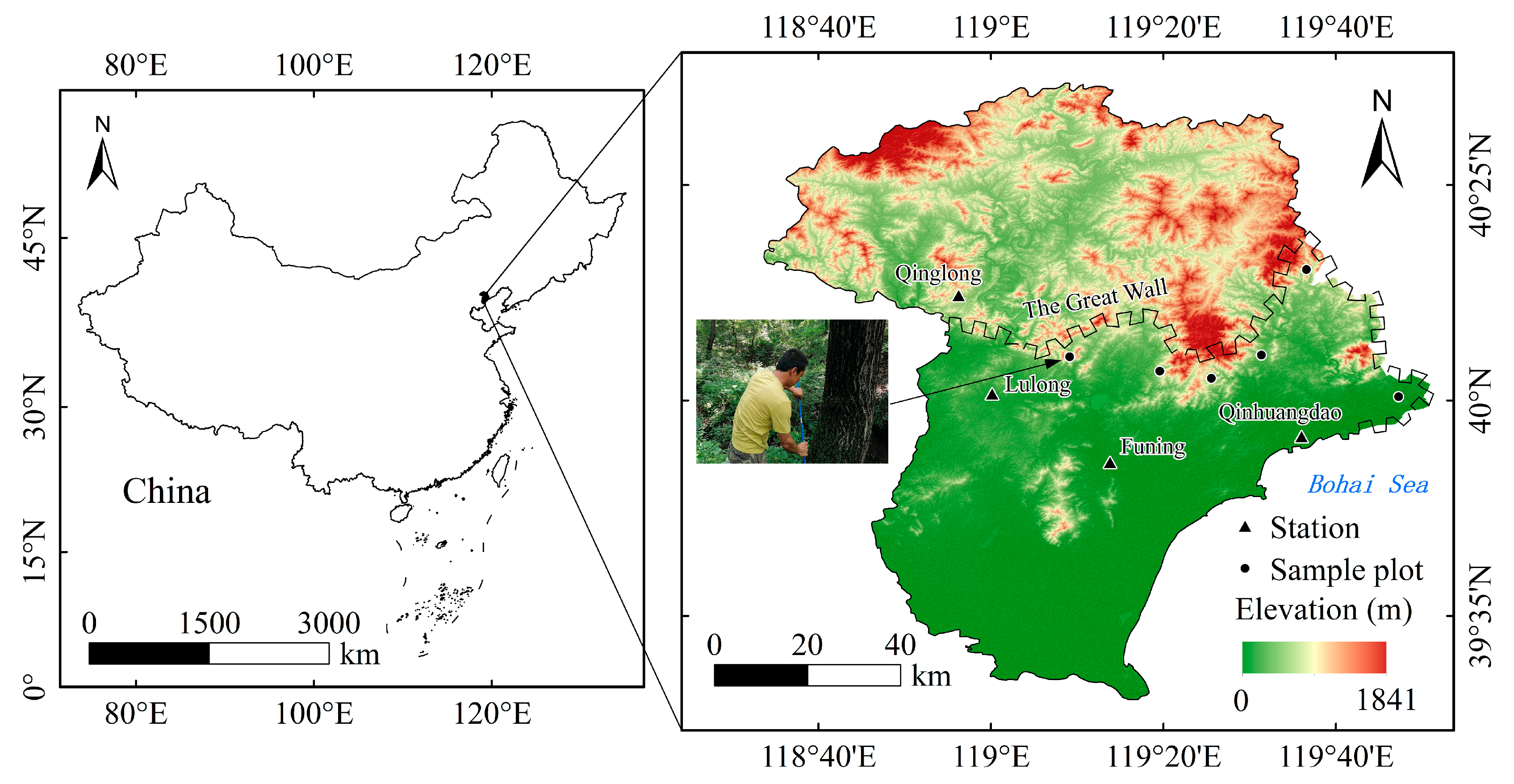
2.1. Study Area

Our study was located in Northern Hebei Province, adjacent to Liaoning (in the Inner Mongolia Provinces along the Great Wall) (Figure 1). The Great Wall was built along the Yanshan Mountains. The south of the Great Wall is an agricultural area, and the north is a pastoral area. Therefore, the study area is characterized as an agriculture and pasture ecotone that is typical of China (adjacent to the North China Plain) [23,24,25]. The annual temperatures range from 7.98 °C to 11.07 °C and the annual precipitation ranges from 388 mm to 1128 mm (Figure 2a). It is cold in winter and hot in summer, with the precipitation concentrated in the summer (Figure 2b). The North China Plain is a typical farming area and has a long history of farming [26]. The area is sensitive to dry–wet changes and is thus an ideal area for the study of the occurrence of droughts and floods resulting from dry–wet changes [27]. In the Yanshan Mountains, with a relatively small population, there are many ancient wild Carya cathayensis trees scattered across the area. The tree-ring width growth of Carya cathayensis is sensitive to climate change and can be used to obtain historical climate data [28].

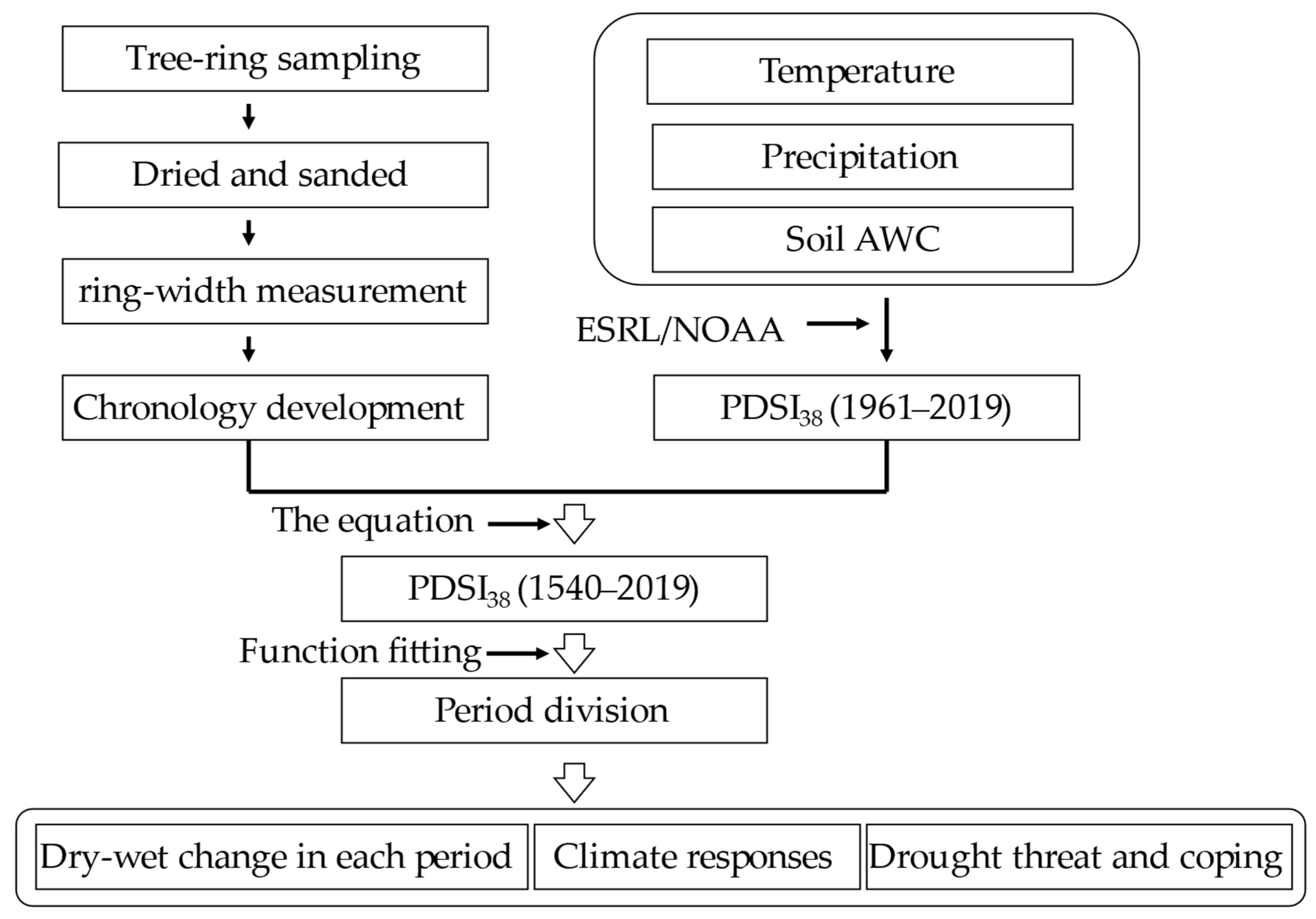
2.2. Tree-Ring Sampling

From 2 July 2018 to 14 September 2018, we obtained 120 Carya cathayensis samples (cores) from six plots in the study area. These sampling points were distributed from west to east along the Yanshan Mountains (the Great Wall), with different elevations at different sampling points, forming a sampling system with several altitude gradients (Figure 1). For each tree, in all plots, two incremental tree-ring cores perpendicular to each other were extracted at a height of 1.2 m above the ground. The cores were sampled from 60 living trees with a diameter at breast height (DBH) > 25 cm, to determine the tree-ring chronologies (Table 1). Four cores (from the total of 120) that were damaged were not considered in our analysis. Firstly, the 116 remaining cores were dried and sanded (to enhance the visibility of the tree growth of the samples). The tree-ring widths were measured using the Velmex ring measurement system [29]. Below, we provide a flowchart to demonstrate the process of data gathering and method of analysis (Figure 3).

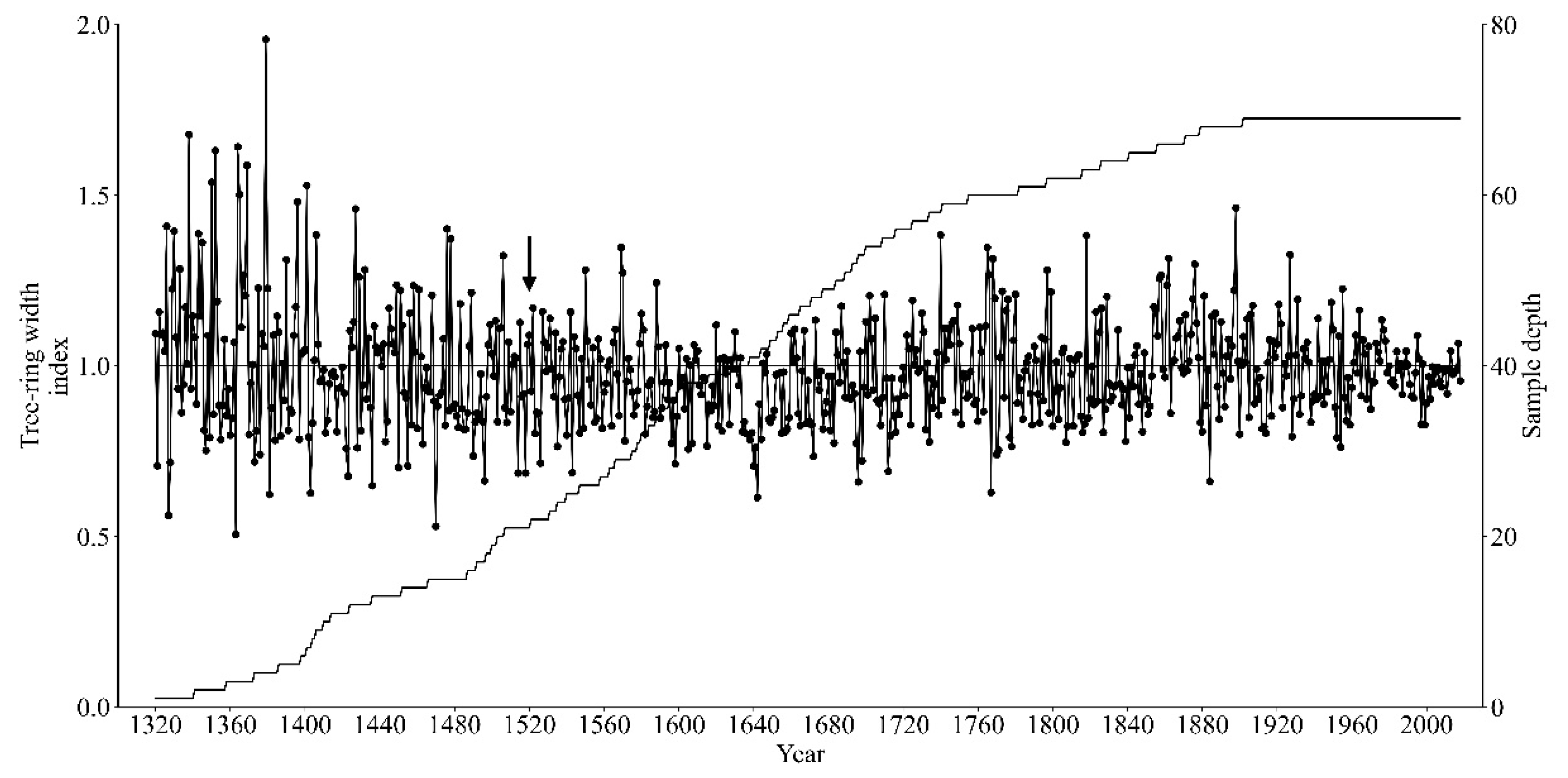
2.3. Chronology Development

All 116 cores were cross-dated by matching the patterns of relatively wide and narrow rings to account for the possibility of ring growth anomalies, such as missing or false rings or measurement errors [30]. The accuracy of the assigned dates regarding errors and measurements was further checked using the computer program COFECHA [31]. The tree-ring series that were poorly correlated with the master series were removed from the final dataset prior to chronology development. The remaining 91 cores were used to obtain the chronological order, using the ARSTAN software [32]. The ring width series were standardized using a smoothing spline with a 50% frequency–response cutoff of 67% of the length of each series. The detrended ring width index series were then pre-whitened by fitting an autoregressive model to remove any autocorrelation effects [33]. Finally, a standard deviation chronology (STD) was developed to reveal the relationship between the climate and tree growth. The mean index (MI) was greater than 0.95, the standard deviation (SD) was 0.03, and the variance of the 1st eigenvector (PCA1) was 43.28% of the STD; this could be used for the growth–climate analysis [34]. The mean series intercorrelation (0.36) and first-order autocorrelation (0.46) of the chronology’s reliability indicated that the STD was sufficient for climate change analysis [35]. The expressed population signal (EPS) (threshold value: 0.85) was determined to reflect a valid time range for the recovery of climate data from a chronology [36]. Therefore, the time span of the STD from 1540 to 2018 was used to analyze the climate change. During this period, the EPS was greater than 0.85 and the sample depth was 25 (Figure 4).

2.4. Statistical Analysis

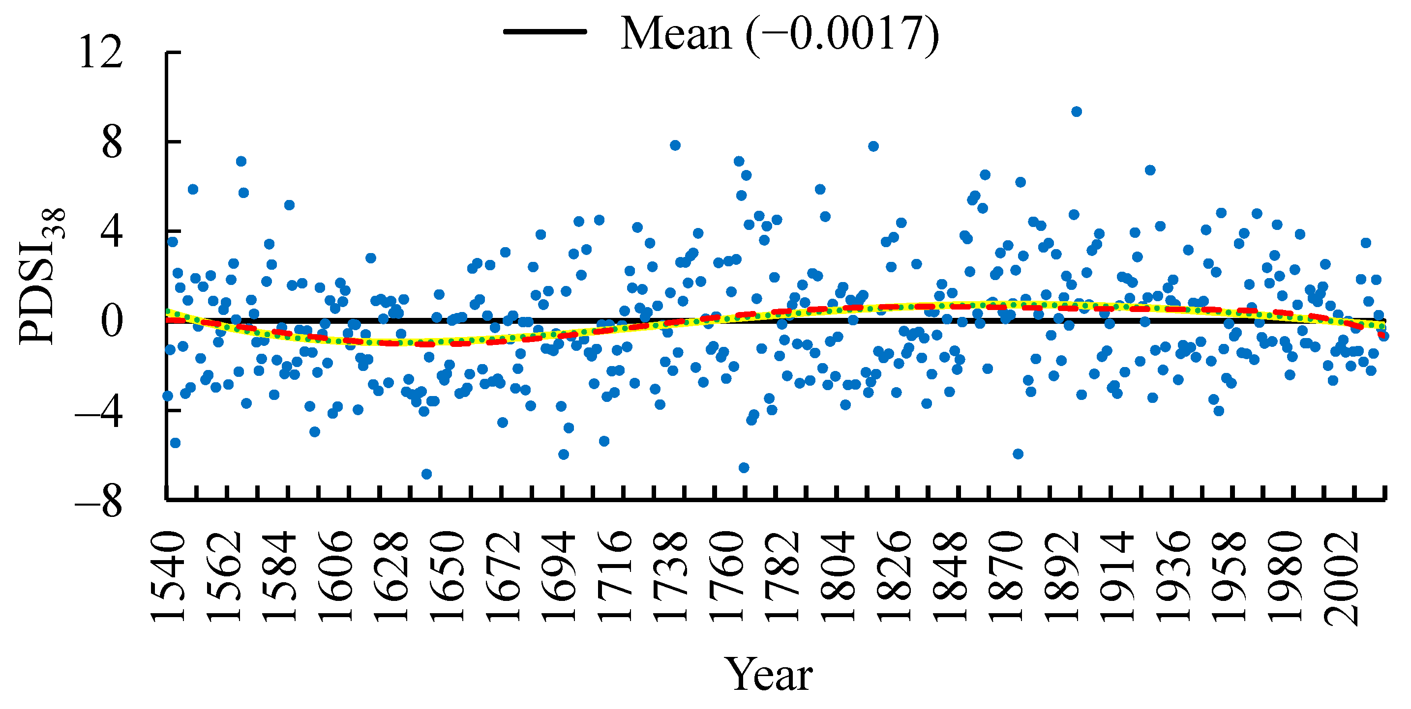
2.4.1. Reconstruction of PDSI38

The temperature and precipitation data were acquired from the Qinglong (118.57° E, 40.25° N), Funing (119.23° E, 39.88° N), Qinhuangdao (119.60° E, 39.93° N), and Lulong stations (118.53° E, 39.53° N) near the Great Wall, from tree-ring sampling spots for 1961–2019. The PDSI38 calculations included three data sets (temperature, precipitation, and the local available water content (AWC) of the soil) for each year (1961–2019) in the study area. Gridded precipitation and temperature data were extracted from the monthly 2.5° × 2.5° dataset compiled by the Climatic Research Unit from 1961 to 2019 [37], combined with the monthly precipitation and temperature data from five selected meteorological stations. The soil AWC data were extracted from the Global Soil Types 1-Degree Grid [38]. Calculations were performed on a 2.5° × 2.5° grid, chosen to achieve a trade-off between the spatial resolution and a reduced number of grid points for data processing. The PDSI38 reconstruction was based on the monthly self-calibrated PDSI (scPDSI) grid data, with a resolution of 2.5° × 2.5° for 1961–2019, which were provided by the Earth System Research Laboratory/National Oceanic and Atmospheric Administration (ESRL/NOAA). The correlation coefficients (Rs) were computed to investigate the relationship between the chronology and climatic factors from 1961 to 2018. The climatic factors included the monthly average temperature and total precipitation from January to December of the current year. The R was also calculated between the PDSI38 and tree-ring width. The relationship between the PDSI38 value and the STD from 1961 to 2018 was revealed using a linear equation. The dependent variable was the PDSI38 and the independent variable was the ring width index of the STD (Equation (1)). The equation passed the test of the leave-one-out model. The reduction of errors (RE) was 0.342, and the Durbin–Watson statistical coefficient (DW) was 1.720 (P (PMT and ST) < 0.05, where PMT represents the value derived using the product mean test and ST represents the sign test) (Table 2). The results indicated that the equation could be used to restore the values of the PDSI38 [39]. Therefore, the PDSI38 values between 1540 and 1960 were computed using Equation (1), based on the tree-ring width of the STD, as follows:
Y = −18.545 + 19.065·x (r = 0.692, R2 = 0.479, R2adj = 0.470, p < 0.01)
where the PDSI38 is represented as Y, the tree-ring width index is represented as x and adjusted R2 is represented as R2adj. The values of the PDSI38 from 1540 to 1960 were computed using Equation (1). The PDSI38 records were derived from the ESRL/NOAA data for 1961–2019. Then, we overlaid the PDSI38 from 1540 to 1960 with the PDSI38 from the ESRL/NOAA for 1961–2019. Finally, a 480-year (from 1540 to 2019) series for the PDSI38 was reconstructed by combining the two sets of results (Figure 5).

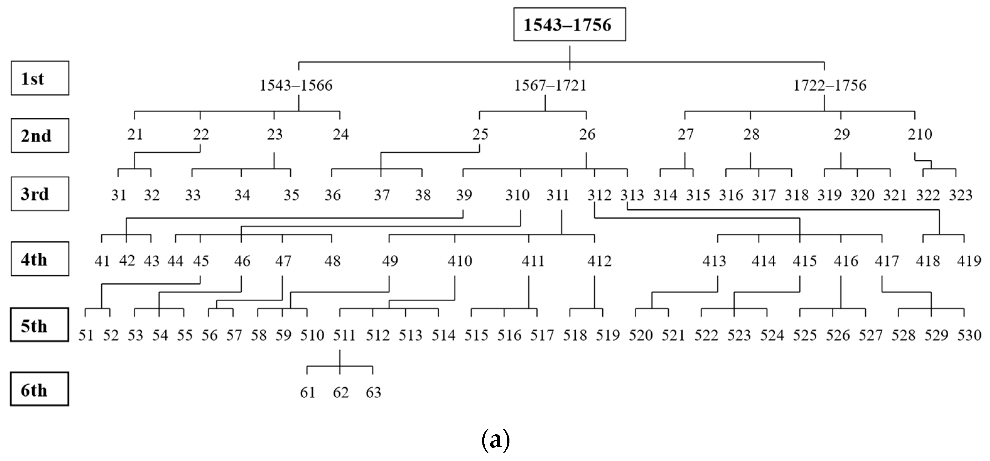
2.4.2. Period Division of the PDSI38 Related to Dry–Wet Changes

Division Using Function Fitting Methods

We used the year as the independent variable and the PDSI38 of each year as the dependent variable for function fitting. If a function fitted well (R2 > 0.6; p < 0.05), it indicated that the PDSI38 change followed the law of the function curve. Based on the fluctuation characteristics of the curve, it could be divided into different dry–wet periods. However, in the 480-year period, the fitting effects of all functions from 1 to 30 times were not satisfactory (R2 < 0.2; p > 0.05). Therefore, using a segmentation fitting method, the 480-year period was divided into different periods for function fitting, and good fitting functions (R2 > 0.6; p < 0.05) were extracted for the different time periods. Based on the changes in the function curves, the variation law of the PDSI38 was analyzed within the different periods. Well-fitting function curves can be used to divide the periodicity of the research object with the change in time. Therefore, the relationships may be used to divide the time series of the research object between the function curve and the mean line [40]. The periodic change in the PDSI38 was applied using the stepwise regression method from the 4th to 6th functions. The functions were selected between the PDSI38 (dependent variable) and the time series (independent variable) for 1540–2019. Firstly, the mean of the PDSI38 was calculated for 1540–2019. Then, the different periods were divided using the intersections between the function curve and the mean line. The mean of three intersections between the three function curves and the mean line was calculated to divide the different periods, because the three function curves from the 4th to 6th functions were similar during the study period. The wet cycle was selected when the function curve was above the mean line. The dry cycle was represented by the curve below the mean line. Finally, the periodic change in the PDSI38 values was divided completely in the first step. When the p values of the three functions were greater than 0.5 (p > 0.05), each period in the first step was divided again, using the same method as in the first step. The next step was carried out until the p value of the function was less than 0.05. The first step was considered as an example, to explain the periodic division of the PDSI38.

Division Process of Function Fitting

The left-most intersection was the year of 1541 between the 4th function curve (from 1540 to 2019) and the mean line (PDSI38 = −0.001). The 5th function was the year of 1545 and the 6th function was the year of 1543. Then, the mean (1543 year) of the three years (1541, 1545, and 1543) was considered as the first point for periodic division. The second point was the year of 1757, and 1992 was the third point (for periodic division, using a similar method). The PDSI38 values were divided into three cycles, from 1540 to 2019, according to the three intersections. The first dry cycle was from 1543 to 1756, because the three function curves (from 4th to 6th) were below the mean line (the three years from 1540 to 1542 were not considered in the study). The first wet cycle was from 1757 to 1992, because the three function curves (from 4th to 6th) were above the mean line during this period. The second dry cycle was from 1993 to 2019. The first step was concluded for the periodic division of the PDSI38 change. The p values of all functions were greater than 0.5. Therefore, a second step was needed for periodic division. Finally, periodic division was performed successively until the 6th step in the first dry period (Figure 6a). The wet period was divided completely by the 5th step (Figure 6b), and by the 2nd step in the second dry period, as there were only 28 years in this period (Figure 6c).

Analysis Methods

The means, STDs, and durations of the PDSI38 were calculated for the average of each period within each of the first dry, the first wet, and the second dry periods, respectively. Regarding the results of the mean PDSI38 for each step, the PDSI38 change of each period was analyzed using the 6th function in order to reveal the periodic characteristics of the dry–wet change. Regarding the results of the STDs of the PDSI38 for each period, the fluctuation law of the PDSI38 was analyzed for each step using the 6th function in order to reveal the periodic characteristics of the dry–wet change. The duration of the periodic dry–wet change was understood in the same way.

3. Results

The chronology was strongly correlated with the temperature and precipitation from June to August of the current year (the year corresponding to climate factors was the same as the year of tree-ring width growth) (p < 0.05 and p < 0.05) (Figure 10a,b), indicating that the tree-ring growth responded very positively to changes in the temperature and precipitation in the active growth period. In addition, the R between the ring width chronology and PDSI38 was 0.692 (p < 0.01). The tree growth was sensitive to dry–wet changes.

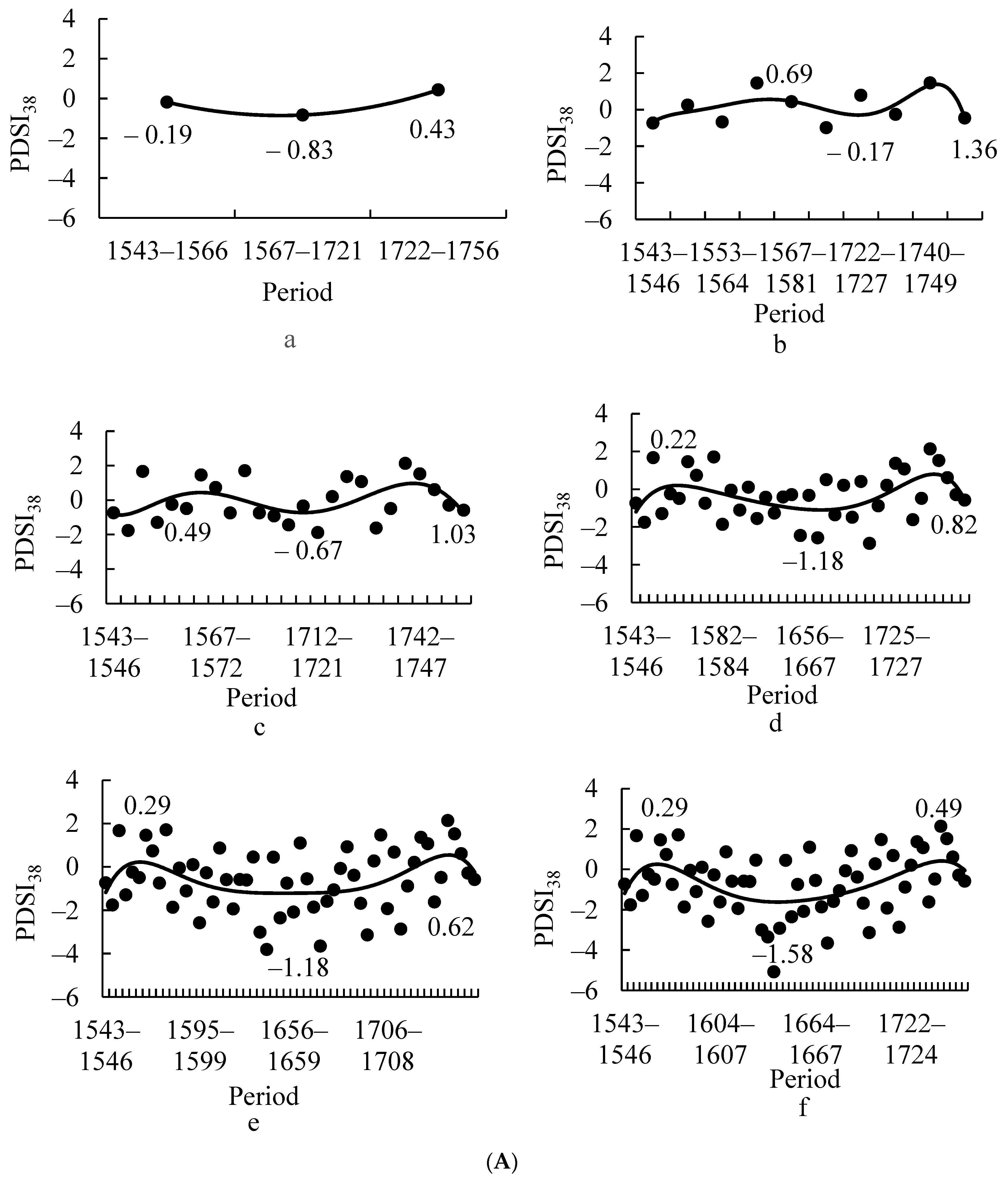
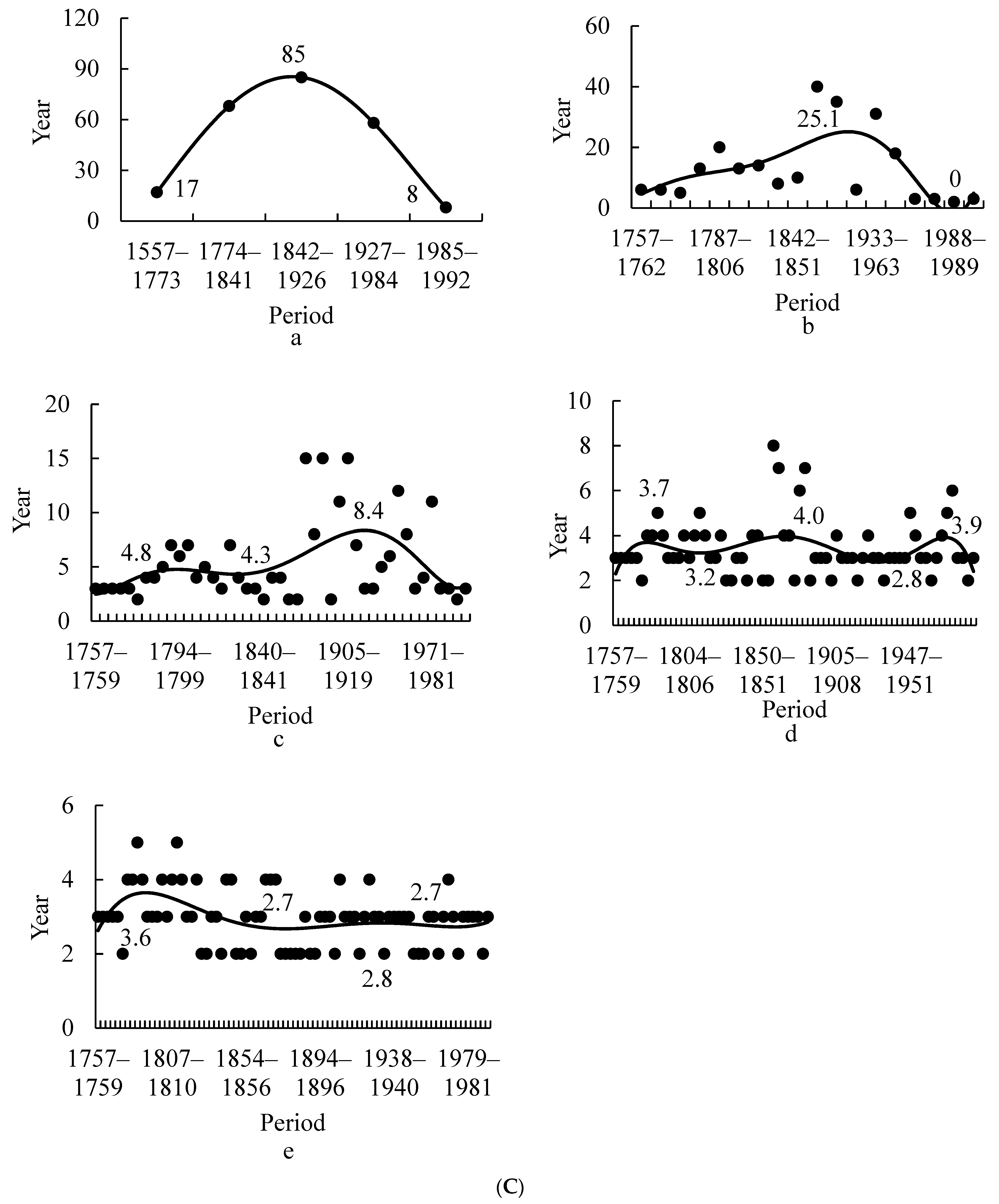
3.1. First Dry Period

3.1.1. Change in the Mean of the PDSI38 in All Periods

The averages of the mean PDSI38 values in all periods were −0.20 (first step), 0.12 (second step), −0.05 (third step), −0.35 (fourth step), −0.58 (fifth step), and −0.69 (sixth step) for all steps, respectively, for the long (the first step), intermediate (the second and third steps), and short (the fourth, fifth, and sixth steps) periods, indicating an initial trend of increasing followed by a decrease. The change range of the PDSI38 was 0.81 [0.12 (maximum)–−0.69 (minimum)], with fluctuations above and below the mean line (−0.001). The results indicated that the regional climate can maintain the relative stability of the dry–wet period, which reflected the region’s potential to become the first agricultural area in China. The SDs of the mean PDSI38 values in all periods were 0.51, 0.85, 1.19, 1.23, 1.43, and 1.54 from the first to the sixth steps, respectively, indicating a gradual increase; thus, the differences between the periods increased gradually, and the fluctuations increased from the long to the short periods. All function curves exhibited a single concave shape; the concavity of the shape increased and the maximum values were found at the curve edges (at 1550–1581 and 1725–1749) from the long to the short periods (Figure 7A). The results indicated that the region had certain wet season characteristics when entering and exiting a dry period. The minimum values occurred in the middle (at 1636–1659) of the curve (Figure 7A), indicating that the strongest drought appeared in the middle of the period.

3.1.2. Change in the Standard Deviation (SD) of the PDSI38 in All Periods

The averages of the SDs of the PDSI38 values in all periods were 24, 23, 22, 22, 19, and 18 from the first to the sixth steps, respectively, indicating a gradual downward trend, and the duration of the dry period decreased from the long to the short periods. The SDs of the PDSI38 values in all periods were 1, 9, 13, 11, 11, and 11 for the first to sixth steps, respectively, with a gradual upward trend, indicating that the dry difference among all periods increased gradually from the long to the short periods. The results indicated that the dry period relieves or even transforms into a wet period in the next period, to maintain the dry–wet balance, when the dry period within one cycle is long. The function curves presented a double concave shape in the intermediate and long periods (Figure 7B(b–d)), indicating that the fluctuations were small at the beginning and the end of the dry period, and the regional climate fluctuated relatively little in the early (approximately 1550–1581) and late periods (approximately 1725–1749) of the dry period. However, the dry fluctuation was the largest in the middle period (approximately 1636–1659) of the dry period, with the most severe droughts (Figure 7B(a–d)), which indicated that the regional climate tended to adjust itself as much as possible to overcome the drought in the long and intermediate periods. In the short periods, the function curves exhibited a single depression (Figure 7B(e,f)), indicating that the region could not change the severe drought conditions during 1633–1645.

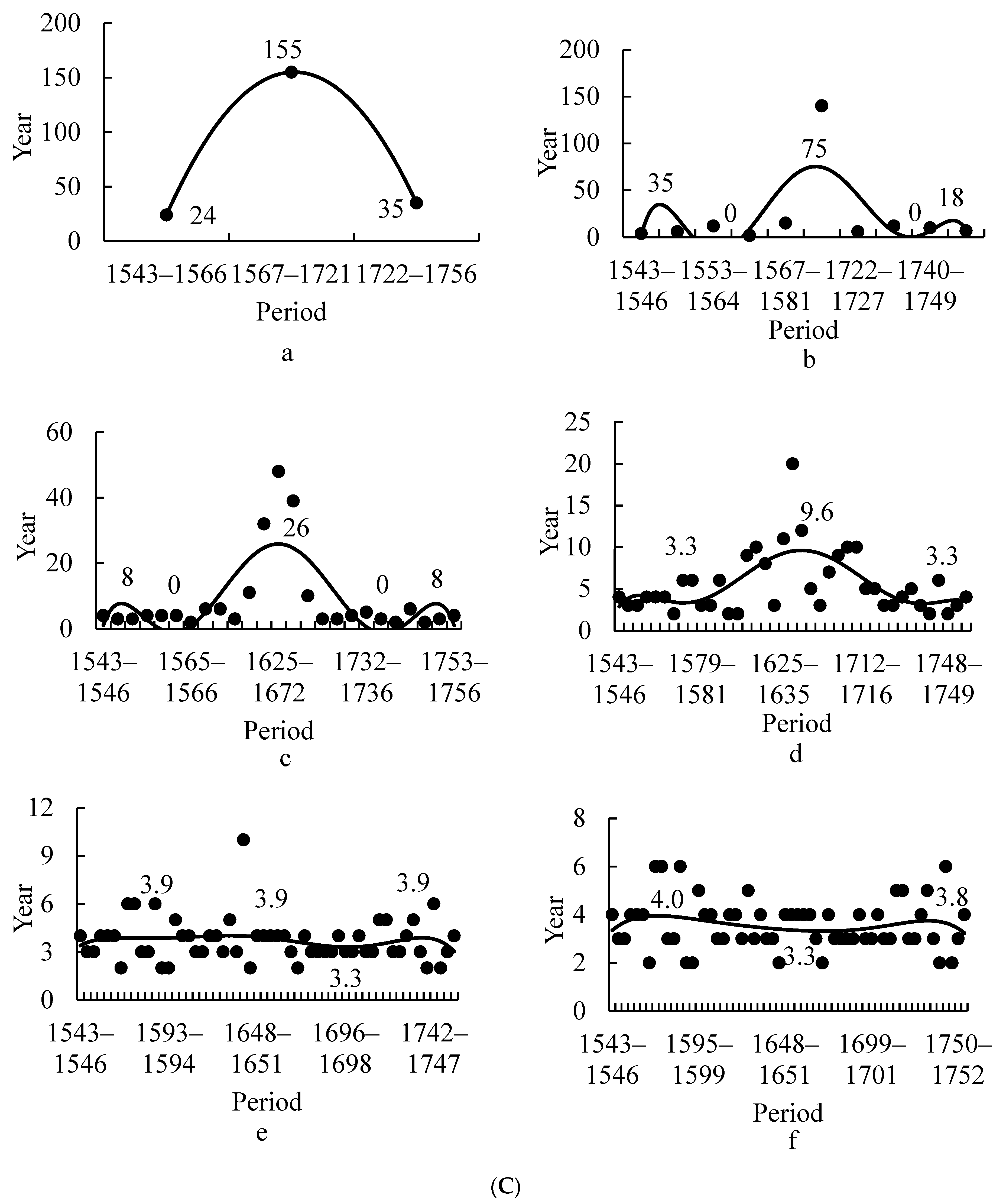
3.1.3. Change in the Duration of the PDSI38 in All Periods

The average durations of all periods were 71, 21, 9, 5, 3.7, and 3.6 years from the first to the sixth steps, respectively. The duration of the long period was 71, those of the intermediate periods were 21 and 9 years, and those of the short periods were 5, 3.7, and 3.6 years. The results were consistent with the historical data, i.e., during this period, disasters had periodic characteristics of 3–5, 20, and 70 years [41], which were influenced by the cyclical changes in the solar activity cycle and the cycle of the El Nino Southern Oscillation (ENSO) [42,43]. The SDs of the duration of the PDSI38 in all periods decreased from 59, 40, 12, 3.6, 1.3, and 1.0 years (from the first step to the sixth step, respectively), indicating that the difference in the duration of each period in the long period was the largest; the difference was only one year for each period in the short period. The dry situation changed once every 3–5 years. The function curves showed a single peak in the intermediate and long periods (Figure 7C(a–d)), indicating that the durations of the different periods were long in the intermediate and long periods. Some short periods with high PDSI38 values were interspersed to adjust the regional climate, so as to reduce the duration of a severe drought as far as possible. However, the function curves fluctuated very little in the short periods (Figure 7C(e,f)), indicating that the droughts were completely contained within the short periods.

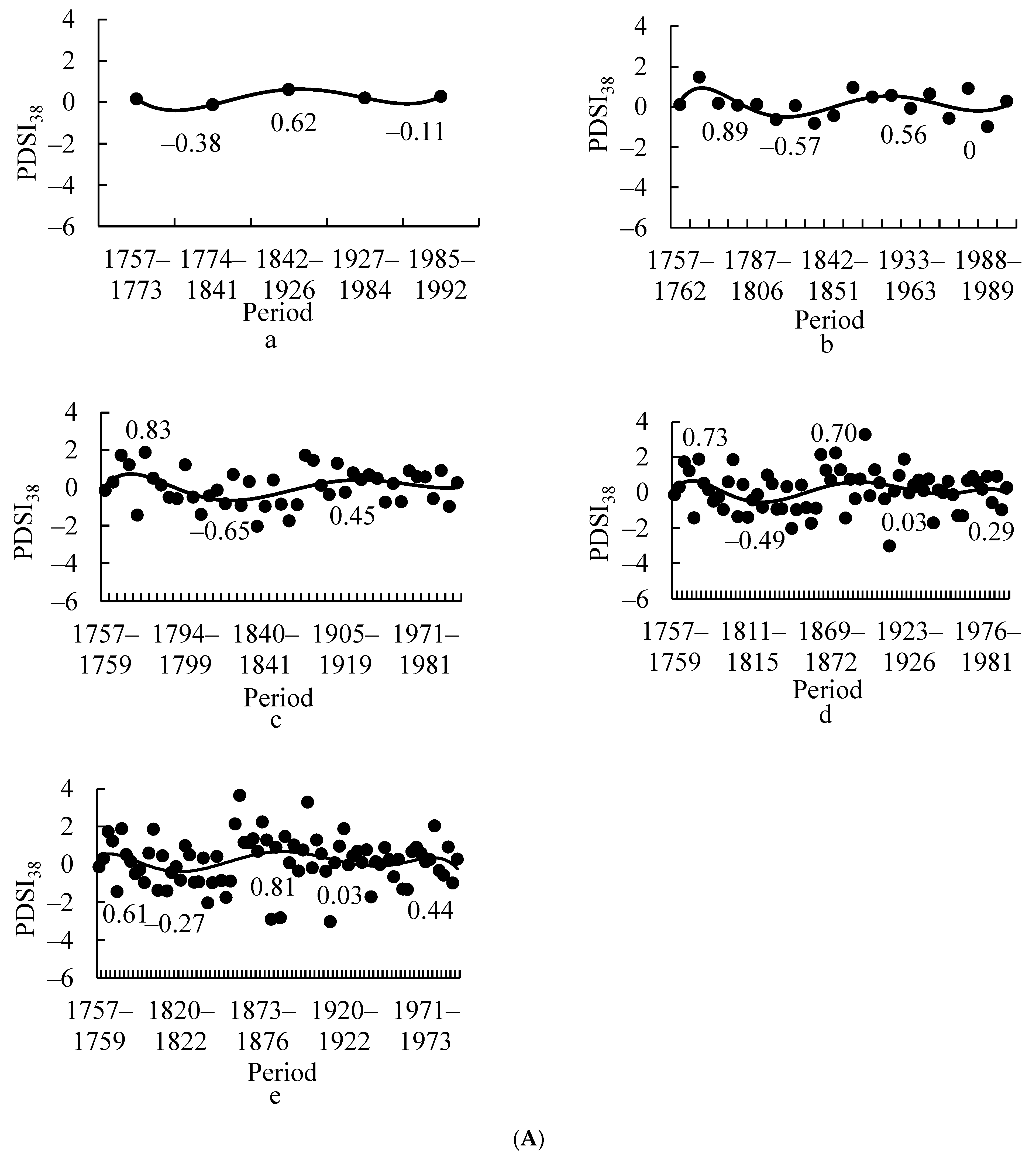
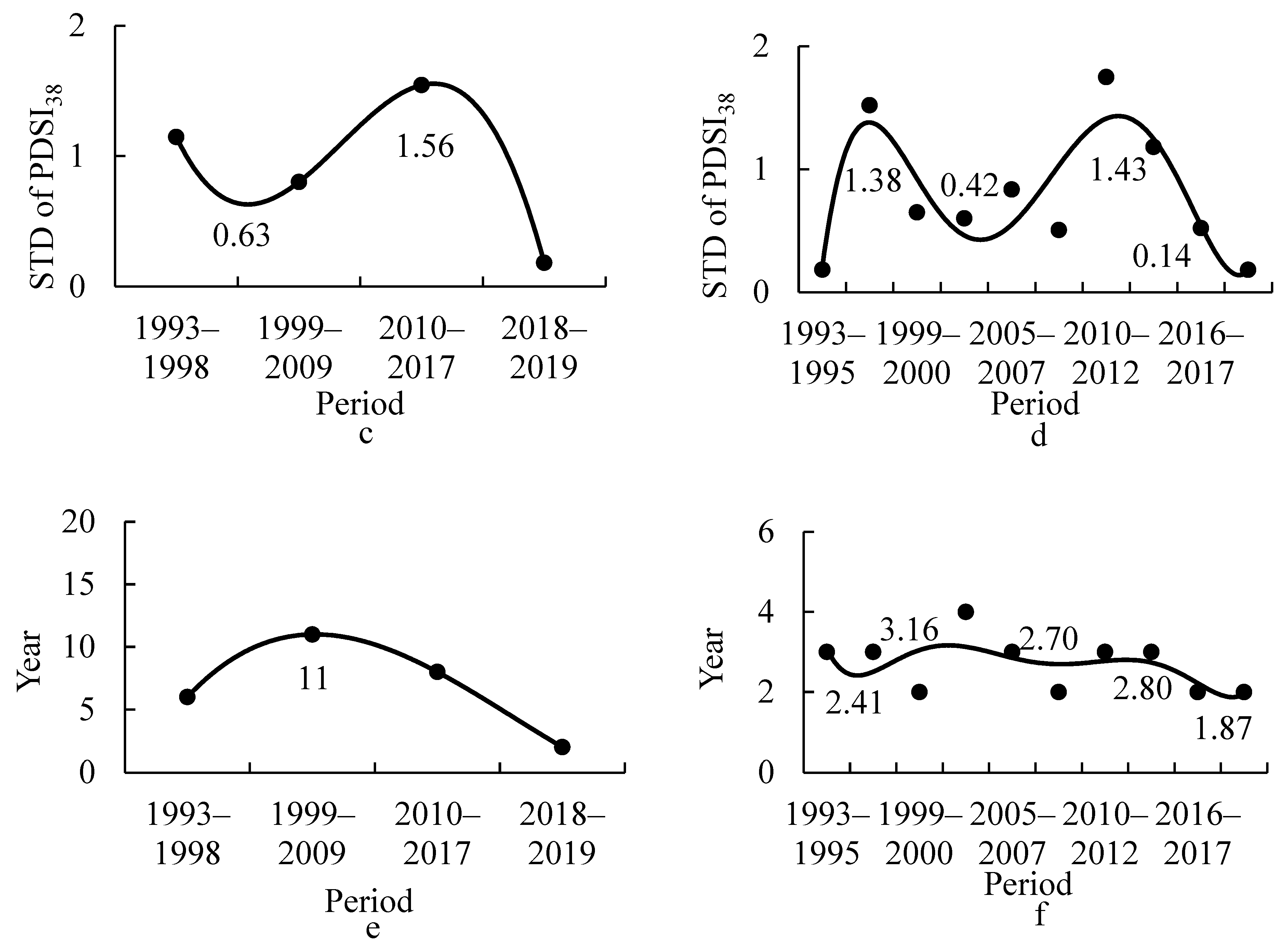
3.2. First Wet Cycle

3.2.1. Changes in the Mean PDSI38 in All Periods

The averages of the mean PDSI38 values in all periods were 0.23, 0.13, 0.05, 0.12, and 0.17 from the first to the fifth steps, respectively. The difference in the PDSI38 was only 0.18 [0.23 (maximum)–0.05 (minimum)] between the long (the first step), intermediate (the second step), and short (the third, fourth, and fifth steps) periods. Notably, all periods were relatively stable. Northern China is one of the most important grain-producing areas in China, and the planting structure is dominated by dry fields. The SDs of the mean PDSI38 in all periods were 0.24, 0.64, 0.95, 1.13, and 1.25 from the first to the fifth steps, respectively, indicating a gradual increase, and the wet difference among all periods became larger as the period became shorter. The function curves were almost double concaves, progressing from the long to the intermediate and short periods (Figure 8A(a–e)), which indicated that the PDSI38 was rather low at the beginning (1807–1839) and end (1938–1955) of the wet period. The regional climate tended to be dry in the early and late stages of the wet period. Meanwhile, the PDSI38 was high in the middle of the period (approximately 1876–1904), which indicated that the flood with the wettest characteristics appeared during the wet period.

3.2.2. Changes in the SD of the PDSI38 in All Periods

The average SDs of the PDSI38 values in all periods were 2.14, 1.94, 1.75, 1.58, and 1.53 from the first to the fifth steps, respectively, with a gradual downward trend, indicating that the wet period decreased from the long period to the short period. However, the SD values of all periods were 0.67, 0.89, 0.94, 0.96, and 0.98 (for the first to fifth steps, respectively), with a gradually increasing trend, indicating that the wet difference between the internal periods increased gradually. The function curves were double concaves from the long to the short periods, and the second concave was relatively flat (Figure 8B(a–e)), indicating that the PDSI38 value fluctuated minimally and was relatively stable during the entire wet period, after a short period of adjustment at the beginning (1763–1768) of this period. The results indicated that the region maintained a relatively stable dry–wet state, which could provide suitable climatic conditions for agricultural production in wet periods.

3.2.3. Change in the Duration of the PDSI38 in All Periods

The average durations of all periods were 47, 13, 5, 3, and 3 years from the first step to the fifth step, respectively. The duration of the long period was 47 years, that of the intermediate period was 13 years, and that of the short period was 3 years. The results were consistent with the changes in the drought and flood disasters in the Han River Basin over the past few hundred years. In addition, during this period, the number of floods (25 times) was greater than the number of droughts (13 times), indicating that the overall climate was relatively humid in this period [44]. The SDs of the duration of the PDSI38 values of all periods decreased from 33, 12, 3.6, and 1.3 to 0.8 years, from the first step to the fifth step, respectively, indicating that the difference in duration was small in the short period. The function curves consisted of a single peak in the long periods (Figure 8C(a)), indicating that the duration was long in the middle stage (1842–1926). The curve had a small single peak at the back (Figure 8C(c)), indicating that the duration of each small period was not notably different in the short period. There was only one small single peak in the function curve in the initial stage of the short cycle, following which the shape was linear (Figure 8C(e)), indicating that the durations were relatively stable during the short cycles.

3.3. Second Dry Period

The function curves for the mean PDSI38 values of all periods consisted of double concaves; however, the right concave was small, indicating an upward trend (Figure 9a,b), illustrating that the regional climate had a certain rectifying effect in the early part of the dry period, which caused the dry conditions to change to normal conditions. The function curve for the SDs of the PDSI38 values of all periods was very complex (Figure 9d), indicating that the dry fluctuation increased at the beginning of the period. The function curve for the duration presented a double-concave shape (Figure 9f), indicating that the ability of the region to achieve climate adjustment and dry rectification was strong as the period began.

4. Discussion

4.1. Climate Responses

The Rs between the monthly average temperature and STD from June to August were 0.35 (JUN, p < 0.01), 0.49 (JUL, p < 0.01), and 0.28 (AUG, p < 0.05), respectively (Figure 10a), indicating that, during the growing season, changes in temperature yielded a positive effect on tree growth [45]. From 1961 to 2019, the average monthly air temperature in the studied area was 22 °C in June, 25 °C in July, and 24 °C in August (Figure 10b). The temperatures were high and the conditions were favorable. The trees began their most active growth period, experiencing increased cell growth and radial expansion, indicating that the active growth period is crucial for tree-ring width growth. The STD was highly correlated with the precipitation from June to August of the current year (p < 0.01 and p < 0.05). The study by Stjepanovic et al. (2018) found that the growth of Carya cathayensis was affected by the precipitation, with significant differences observed when there was a lack of rainfall (p < 0.05) [46]. A drought during the growth period also contributed to reduced growth. The precipitation was highest in June, July, and August, with 100 mm, 231 mm, and 175 mm of rainfall, respectively (Figure 2b). The period was characterized by both high heat and high water availability in the region. Based on the findings of Li et al. (2016), trees grow better at higher temperatures when adequate water is available [45]. During the growth season, the tree rings widen in response to the temperature and rainfall. Moreover, there was a significant (p < 0.05) correlation between February’s mean temperature and the ring width index. According to the lag characteristics of trees when adapting to cold conditions [47], the growth of the trees was related to the coldest temperature during January (−7.24 °C). To cope with low temperatures, the trees had to use their stored resources, which resulted in less growth. The Rs values between the STD and either the temperature or precipitation did not reach significant levels (p > 0.05), as shown in Figure 10a,b. Thus, the lack of extreme heat limited the growth of the trees. During the previous year’s growing season, the trees accumulate storage reserves, utilizing carbon allocation to endure the harsh non-growing season [48]. Therefore, the cold temperatures (except during the coldest month) and low rainfall did not have a significant impact. The R value of 0.692 between the STD and PDSI38 (p < 0.01) indicated that tree growth requires less water in agricultural and pastoral ecoregions [49], due to a combination of increased precipitation and the accelerated depletion of the water supply by warmer temperatures [48]. Thus, the water availability is influenced by these factors.

4.2. Drought Threat

There is one additional step in the first dry period (consisting of six steps) (Figure 6b) compared to the first wet period (consisting of five steps) (Figure 6c), and the number of cycles in each step of the first wet period was greater than that in the corresponding step of the first dry period (Figure 6b,c). The results indicated that droughts were relatively more concentrated and prominent, while floods were relatively scattered; thus, the floods were less severe than the droughts. The regional climate could not be effectively regulated in some periods, which could have had a serious impact on agriculture when severe droughts occurred. For example, the most severe drought in the first period occurred between 1640 and 1642, with the mean PDSI38 value being only −4.68. Therefore, we could conclude that the region was experiencing an extreme drought at that time, when the value of the PDSI38 was <−4 [50]. In addition, the mean PDSI38 values of the two periods (1633–1635 and 1636–1639) were −1.71 and −3.35, respectively, which indicated that the droughts were mild and severe in these two periods [50]. According to historical records, this time period coincided with the reign of the late Ming Dynasty. During this period, successive droughts caused agricultural failures, resulting in a lack of agricultural production in Northern China [51]. In the first two drought periods (1633–1635 and 1636–1639), agricultural production was reduced significantly, and the population consumed all of the available food. At the end of the Ming Dynasty in 1644, the most severe drought (1640–1642) occurred in the region; there was no food to eat, and severe starvation and social unrest occurred [52]. Then, the Qing Dynasty gradually began its reign over China. Notably, there was no drought in China between 1646 and 1647 [53]. This was roughly consistent with the results of our study (1646–1647: PDSI38 = 0.44, normal) [54]. During this period, i.e., around the middle of the 17th century, extreme droughts occurred in many parts of the world. For example, extreme droughts occurred in South Asia in 1615–1626 [55], South America in 1620–1630 [56], Europe in 1625–1632 [57,58], Australia in 1636–1645 [59], South Africa in 1640–1660 [60], and North America in 1655–1675 [61]. Therefore, many parts of the world experienced severe droughts in different years during this stage (1633–1642) (or near this stage).

4.3. Strategies to Address Severe Droughts

In the first dry period, from 1633 to 1645, four periods (1633–1635 (PDSI38 = −1.71), 1636–1939 (PDSI38 = −3.35), 1640–1642 (PDSI38 = −4.68), and 1643–1645 (PDSI38 = −2.92)) with low PDSI38 values occurred successively, and severe droughts lasted 13 years. We speculate that there will be a severe drought in the early part of the 22nd century, based on the Chinese calendar of dry–wet changes that we have studied, where the duration of the first drought period was 214 years. In the middle of the period, the most severe drought occurred, with a half period of 108 years. The time point at which the second drought period began was 1992. According to this time point, it is speculated that 2100 will be the driest year in the future, occurring 108 years later. At the same time, according to the IPCC [62], at the end of the 21st century, sudden changes in climate factors such as temperature and precipitation may cause extreme droughts on a large scale throughout the world. Therefore, appropriate risk management measures should be planned accordingly. In addition, building water conservancy facilities and storing water and grain would provide active assistance in locations where severe droughts may occur in the future. The agricultural planting scheme should also be changed according to the actual dry–wet conditions in different regions. For example, according to historical records, there were 11 droughts in Sichuan during 1625–1645, with the average value of the PDSI38 being −2.03 for all periods, based on the results of this study (the lowest of the research years). In order to survive this difficult period, the region was forced to transition from paddy fields to dry fields [63]. During 1646–1682, grain production increased gradually; finally, it led to large harvests for three consecutive years during 1680–1682 [63]. Therefore, some traditional rice-producing areas changed to dry land and planted food crops with higher yields. In the Yangtze River Basin, from 1633 to 1645, drought and wind disasters reached an average annual frequency of 2.6 times. Under the pressure of such drastic climate changes, millions of people moved from the Yangtze River Basin to the south of the Nanling Mountains (Pearl River Basin) [64], indicating that the impact of the drought on Guangdong and Guangxi was small. During this period, other tropical regions in the world were also insignificantly affected by extreme droughts [65,66,67]. Since China once purchased rice from the Indochina Peninsula and extreme droughts did not occur simultaneously worldwide, the time differences of the drought period could be used when purchasing different grains from different regions. For example, an extreme drought in South America (1620–1630) occurred earlier than that in North America (1655–1675). Owing to this asynchronism with North America, South America could have first purchased grains from South America; then, when North America entered the drought period, North America could have purchased grains from South America. Australia, South Asia, Europe, and East Asia could also have followed this method. In addition, the droughts in tropical areas are not serious; thus, the surplus produce from these regions could be exported to other parts of the world. Therefore, the threat of extreme drought can be minimized through global cooperation.

4.4. Period of Dry–Wet Change

The dry–wet change occurs in a cycle of 12 years or multiples of 12, and the first wet period (1757–1992) lasted a total of 236 years. By merging the period of 1985–1992 with the previous period of 1927–1984, we initially divided the first wet period into four periods (long cycle) (Figure 6c). The average length of the initial wet period’s long intervals was 59 years, which was nearly a 60-year interval. The average duration (13 years) of all intermediate periods (the fourth step) in the initial wet period was comparable to the 12-year duration of the initial wet period. However, the duration of each interval in the dry period was slightly shorter than 12 years. The first dry period lasted 214 years (1543–1756), which is 26 years shorter than 240 years, and each period lasted 2 years less than two 12-year periods. The average length of the long periods (first step) during the first dry period was 71 years, one year less than the 72-year period of the sum of the 60- and 12-year periods. The average length of all intermediate periods (third step) during the first dry period was 9 years, or 3 years less than the 12-year average. These outcomes could reflect a 12-year change that is influenced by both the lowest point of the solar cycle and ENSO [68,69]. The dry–wet change over 60 years might be impacted by the Pacific Decadal Oscillation (PDO) [70], and the 120-year change could be linked to centennial-scale solar cycles [71]. Thus, the years of the dry–wet change can be roughly inferred using a 12-year or multiple 12-year cycle. The duration of the short period was 3–5 years in all dry and wet periods; this finding was in agreement with several previous studies. For example, the droughts in the region presented a 4-year periodic oscillation from 1961 to 2009 [72]. The main period of dry–wet changes in China lasted 4.4 years [73]. Even in Southern Africa, floods also occurred in one period with four years [74]. These periodic changes are all related to the El Nino and La Nina phenomena [75]. Therefore, that the shortest period of dry–wet changes in the region, and even in China, lasts 3–5 years indicates that China is deeply affected by these two phenomena.

5. Conclusions

The tree-ring data of Carya cathayensis were used to establish a chronology and restore the PDSI3 of the ecotone between farming and animal husbandry along the Great Wall for the period of 1540–2019. The stepwise function method was used to study the periodicity of the dry–wet changes. There were two dry cycles and one wet cycle during the 477 years considered in this study. Each dry–wet period was divided into different levels, including long (decades), intermediate (10 years), and short periods (several years, less than 10 years). In the first dry period, the change range of the PDSI38 value was not high for all periods (from the first to the fifth steps), indicating that the region maintained a stable dry–wet status. However, in the short period (the sixth step), there were periods of severe drought (1633–1645). In the first wet period, the fluctuations in the PDSI38 values were very small in each individual period. The capacity for the regulation of regional floods was stronger than that of regional droughts, and the values of the PDSI38 changed smoothly during this period; thus, the conditions were favorable for agricultural production. In the second drought period, only the initial stage of the drought was analyzed. During this period, the changes in the dry–wet period were corrected and, thus, the region maintained a relatively stable status. Compared with floods, droughts pose a greater threat, not only in China but throughout the entire world. Therefore, we should plan and implement effective measures to prepare for the severe droughts that may occur in the future. Notably, the durations of the long, intermediate, and short periods of the dry–wet periods were consistent with those indicated in a 12-year or multiple 12-year cycle; thus, the information in the sexagenary can be used to predict the occurrence of droughts and floods in China.

Supplementary Materials

The following supporting information can be downloaded at: https://www.mdpi.com/article/10.3390/ijgi13060191/s1, Table S1: The numbers in the Figure 6a indicate the years of the cycles in the first dry cycle (1540–1756); Table S2: The numbers in the Figure 6b indicate the years of the cycles in the first wet cycle (1756–1992) and the Figure 6c (the second dry cycle (1993–2019)). This study’s supplementary materials can be available from the author upon.

Author Contributions

Conceptualization, methodology, and writing-original draft preparation, Xiaodong Wang; methodology, investigation, and writing-original draft preparation, Xiaoqiang Li; formal analysis, Yujia Song; investigation, Yu An; editing and project administration, Xiaohui Liu. All authors have read and agreed to the published version of the manuscript.

Funding

This research was funded by Joint Funds of the National Natural Science Foundation of China (U2243230); the National Natural Science Foundation of China (42230516); Technology Development Program of Jilin Province (20230203003SF); and Natural Science Foundation of Changchun Normal University (CSJJ2022008ZK).

Data Availability Statement

The data presented in this study are available from the author upon reasonable request.

Acknowledgments

The authors would like to thank the anonymous reviewers and handling editors for their constructive comments.

Conflicts of Interest

The authors declare no conflict of interest.

References

  1. Hu, Z.Y.; Zhou, J.J.; Zhang, L.L.; Wei, W.; Cao, J.J. Climate dry-wet change and dry evolution characteristics of different dry-wet areas in northern China. Acta Ecol. Sin. 2018, 38, 1908–1919, (In Chinese with English Abstract). [Google Scholar]
  2. Misra, V.; Solomon, S.; Mall, A.K.; Prajapati, C.P.; Hashem, A.; Allah, E.F.; Ansari, M.I. Morphological assessment of water stressed sugarcane: A comparison of waterlogged and dry affected crop. Saudi J. Biol. Sci. 2020, 27, 1228–1236. [Google Scholar] [CrossRef]
  3. Wu, J.F.; Chen, X.H. Spatiotemporal trends of dryness/wetness duration and severity: The respective contribution of precipitation and temperature. Atmos. Res. 2019, 216, 176–185. [Google Scholar] [CrossRef]
  4. Yu, X.F.; Wang, Y.; Yu, S.Y.; Kang, Z.H. Synchronous droughts and floods in the southern Chinese Loess Plateau since 1646 CE in phase with decadal solar activities. Glob. Plant Change 2019, 183, 103033. [Google Scholar] [CrossRef]
  5. Huang, Q.Z.; Zhang, Q.; Singh, V.P.; Shi, P.J.; Zheng, Y.J. Variations of dryness/wetness across China: Changing properties, drought risks, and causes. Glob. Planet Change 2017, 115, 1–12. [Google Scholar] [CrossRef]
  6. Peng, Y.; Long, S.F.; Ma, J.W.; Song, J.Y.; Liu, Z.W. Temporal-spatial variability in correlations of drought and flood during recent 500 years in Inner Mongolia, China. Sci. Total Environ. 2018, 633, 484–491. [Google Scholar] [CrossRef]
  7. Cheng, Q.P.; Gao, L.; Zuo, X.A.; Zhong, F.L. Statistical analyses of spatial and temporal variabilities in total, daytime, and nighttime precipitation indices and of extreme dry/wet association with large-scale circulations of Southwest China, 1961–2016. Atmos. Res. 2019, 219, 166–182. [Google Scholar] [CrossRef]
  8. Manoj, V.G.; Jain, K. Unravelling the teleconnections between ENSO and dry/wet conditions over India using nonlinear Granger causality. Atmos. Res. 2021, 247, 105168. [Google Scholar]
  9. Melsen, L.A.; Teuling, A.J.; Torfs, P.J.J.F.; Zappa, M.; Mizukami, N.; Mendoza, P.A.; Clark, M.P.; Uijlenhoet, R. Subjective modeling decisions can significantly impact the simulation of flood and drought events. J. Hydrol. 2019, 568, 1093–1104. [Google Scholar] [CrossRef]
  10. Hao, X.Y.; Wei, H.; Lam, S.K.; Li, P.; Zong, Y.Z.; Zhang, D.S.; Li, F.Y. Enhancement of no-tillage, crop straw return and manure application on field organic matter content overweigh the adverse effects of climate change in the arid and semi-arid Northwest China. Agric. For. Meteorol. 2020, 295, 108199. [Google Scholar] [CrossRef]
  11. Xu, X.C.; Ge, Q.S.; Zheng, J.Y.; Liu, C.W. Reviews of agricultural drought risk assessment. Agric. Res. Arid. Areas 2010, 6, 263–270, (In Chinese with English Abstract). [Google Scholar]
  12. Shi, W.J.; Liu, Y.T.; Shi, X.L. Contributions of climate change to the boundary shifts in the farming-pastoral ecotone in northern China since 1970. Agric. Syst. 2018, 161, 16–27. [Google Scholar] [CrossRef]
  13. Wang, T.F.; Su, B.D.; Zhai, J.Q.; Jiang, T.; Wen, S.S. Variation of drys in Luanhe river basin, 1961–2012. J. Arid. Land Resour. Environ. 2015, 29, 180–185, (In Chinese with English Abstract). [Google Scholar]
  14. Jia, Y.Q.; Zhang, B. Spatio-temporal changes of the extreme drought and wet events in Northern China from 1960 to 2016. J. Nat. Resour. 2019, 34, 1543–1554, (In Chinese with English Abstract). [Google Scholar]
  15. Ma, Z.G.; Dan, L.; Hu, Y.W. The extreme dry/wet events in northern China during recent 100 years. J. Geogr. Sci. 2004, 3, 275–281. [Google Scholar]
  16. Ma, Z.G.; Huang, G.; Gan, W.Q.; Chen, M.L. Multi-Scale temporal characteristics of the dryness /wetness over northern China during the last century. Chin. J. Atmos. Sci. 2005, 29, 671–681, (In Chinese with English Abstract). [Google Scholar]
  17. Xiao, L.B.; Fang, X.Q.; Ye, Y. Reclamation and revolt: Social responses in Eastern Inner Mongolia to flood/dry-induced refugees from the North China Plain 1644–1911. J. Arid. Environ. 2013, 88, 9–16. [Google Scholar] [CrossRef]
  18. Gao, S.; Zhou, T.; Yi, C.X.; Shi, P.J.; Fang, W.; Liu, R.S.; Liang, E.Y.; Camarero, J.J. Asymmetric impacts of dryness and wetness on tree growth and forest coverage. Agric. For. Meteorol. 2020, 288–289, 107980. [Google Scholar] [CrossRef]
  19. Klippel, L.; George, S.S.; Buntgen, U.; Krusic, P.J.; Esper, J. Differing pre-industrial cooling trends between tree rings and lower-resolution temperature proxies. Clim. Past 2020, 16, 729–742. [Google Scholar] [CrossRef]
  20. Maxwell, J.T.; Harley, G.L.; Matheus, T.J.; Strange, B.M.; Van Aken, K.; Au, T.F.; Bregy, J.C. Sampling density and date along with species selection influence spatial representation of tree-ring reconstructions. Clim. Past 2020, 5, 1901–1916. [Google Scholar] [CrossRef]
  21. Ziaco, E.; Miley, N.; Biondi, F. Reconstruction of seasonal and water-year precipitation anomalies from tree-ring records of the southwestern United States. Palaeogeogr. Palaeoclimatol. Palaeoecol. 2020, 547, 109689. [Google Scholar] [CrossRef]
  22. Yadava, A.K.; Misra, K.G.; Singh, V.; Misra, S.; Sharma, Y.K.; Kotlia, B.S. 244-YEAR long tree-ring based drought records from Uttarakhand, western Himalaya, India. Quat. Int. 2021, 599–600, 128–137. [Google Scholar] [CrossRef]
  23. Li, S.J.; Sun, Z.G.; Tan, M.H.; Guo, L.L.; Zhang, X.B. Changing patterns in farming pastoral ecotones in China between 1990 and 2010. Ecol. Indic. 2018, 89, 110–117. [Google Scholar] [CrossRef]
  24. Lin, C.C.; Wang, K.; Sun, Y.M. Study on the change of temperature time series in medium section of agro-pastoral ectone of Northern China during the last 60 years. Acta Agrestia Sin. 2016, 4, 747–753, (In Chinese with English Abstract). [Google Scholar]
  25. Zhou, Y.M.; Zhang, A.; Zhao, X.Y. Analysis of vulnerable characteristics in Chinese northern farming-pastoral region based on coordinated regional downscaling experiment. Acta Sci. Nat. Univ. Pekin. 2017, 53, 1099–1107, (In Chinese with English Abstract). [Google Scholar]
  26. Shelach-Lavi, G.; Tu, D.D. Food, pots and socio-economic transformation: The beginning and intensification of pottery production in North China. Archaeol. Res. Asia 2017, 12, 1–10. [Google Scholar] [CrossRef]
  27. Zhai, X.J.; Huang, D.; Tang, S.M.; Li, S.Y.; Guo, J.X.; Yang, Y.J.; Liu, H.F.; Li, J.S.; Wang, K. The emerge of metabolism in different ecosystems under the same environmental conditions in the agro-pastoral ecotone of northern China. Ecol. Indic. 2017, 74, 198–204. [Google Scholar] [CrossRef]
  28. Stokes, M.; Harlan, T.; Harris, M.; Storey, J.B. Datability of pecan tree ring. HortScience 1995, 30, 523–524. [Google Scholar] [CrossRef]
  29. Velmex, Inc. The Velmex “TA” System for Research and Non-Contact Measurement Analysis; Velmex Inc.: Bloomfield, NY, USA, 1992. [Google Scholar]
  30. Fritts, H.C. Tree Rings and Climate; Academic Press: New York, NY, USA, 1976. [Google Scholar]
  31. Holmes, R. Computer assisted quality control. Tree-Ring Bull. 1983, 43, 69–78. [Google Scholar]
  32. Camarero, J.J.; Martin, E.; Gil-Pelegrin, E. The impact of a needleminer (Epinotia subsequana) outbreak on radial growth of silver fir (Abies alba) in the Aragon Pyrenees: A dendrochronological assessment. Dendrochronologia 2003, 21, 3–12. [Google Scholar] [CrossRef]
  33. Cook, E.R.; Kairiukstis, L.A. Methods of Dendrochronology: Applications in the Environmental Sciences; Kluwer Academic Publishers: Dordrecht, The Netherlands, 1990. [Google Scholar]
  34. Helama, S.; Begin, Y.; Vartiainen, M.; Peltola, H.; Kolstrom, T.; Merilainen, J. Quantifications of dendrochronological information from contrasting microdensitometric measuring circumstances of experimental wood samples. Appl. Radiat. Isot. 2012, 70, 1014–1023. [Google Scholar] [CrossRef]
  35. Davi, N.K.; Jacoby, G.C.; Wiles, G.C. Boreal temperature variability inferred from maximum latewood density and tree-ring width data, Wrangell Mountain region, Alaska. Quat. Res. 2003, 60, 252–262. [Google Scholar] [CrossRef]
  36. Wigley, T.; Briffa, K.R.; Jones, P.D. On the average value of correlated time series, with applications in dendroclimatology and hydrometeorology. J. Appl. Meteorol. Climatol. 1984, 23, 201–213. [Google Scholar] [CrossRef]
  37. Dai, A.G. Drought under global warming: A review. Wiley Interdiscip. Rev. Clim. Change 2011, 2, 45–65. [Google Scholar] [CrossRef]
  38. Zobler, L. Global Soil Types, 1-Degree Grid; Oak Ridge National Laboratory Distributed Active Archive Center: Auckland, New Zealand, 1999. [Google Scholar]
  39. Fan, Z.X.; Brauning, A.; Tian, Q.H.; Yang, B.; Cao, K.F. Tree ring recorded May-August temperature variations since A.D. 1585 in the Gaoligong Mountains, southeastern Tibetan Plateau. Palaeogeogr. Palaeoclimatol. Palaeoecol. 2010, 296, 94–102. [Google Scholar] [CrossRef]
  40. Cromer, T.L. A periodicity threshold theorem for a volterra integral equation. Appl. Anal. 1986, 21, 1–8. [Google Scholar] [CrossRef]
  41. Yao, S.Y. The geographical distribution of floods and droughts in Chinese history, 206 B.C.-A.D. 1911. Far East. Q. 1943, 4, 357–378. [Google Scholar]
  42. Sun, J.Q.; Wang, X.J.; Yin, Y.X.; Shahid, S. Analysis of historical drought and flood characteristics of Hengshui during the period 1649–2018: A typical city in North China. Nat. Hazards 2021, 108, 2081–2099. [Google Scholar] [CrossRef]
  43. Liu, X.Y.; Li, D.L.; Wang, J.D. Spatiotemporal characteristics of dry over China during 1961–2009. J. Desert Res. 2012, 32, 473–483, (In Chinese with English Abstract). [Google Scholar]
  44. Zhang, X.D.; Ren, G.Y.; Yang, Y.D.; Bing, H.; Hao, Z.X.; Zhang, P.F. Extreme historical droughts and floods in the Hanjiang River Basin, China, since 1426. Clim. Past 2022, 18, 1775–1796. [Google Scholar] [CrossRef]
  45. Li, Y.J.; Wang, S.Y.; Niu, J.J.; Fang, K.Y.; Li, X.L.; Li, Y.; Bu, W.L.; Li, Y.H. Climate-adial growth relationship of Larix principis-upprechtii at different altitudes on Luya Mountain. Acta Ecol. Sin. 2016, 36, 1608–1618, (In Chinese with English Abstract). [Google Scholar]
  46. Stjepanovic, S.; Matovic, B.; Stojanovic, D.; Lalic, B.; Levanic, T.; Orlovic, S.; Gutalj, M. The Impact of Adverse Weather and Climate on the Width of European Beech (Fagus sylvatica L.) Tree Rings in Southeastern Europe. Atmosphere 2018, 9, 451. [Google Scholar] [CrossRef]
  47. Zeng, L.B.; Wang, X.P.; Cheng, J.F.; Lin, X.; Wu, Y.L.; Yin, W.L. Alpine timberline ecotone tree growth in relation to climatic variability for Picea crassifolia forests in the middle Qilian Mountains, northwestern China. J. Beijing For. Univ. 2012, 34, 50–56, (In Chinese with English Abstract). [Google Scholar]
  48. Lockwood, B.R.; Leblanc, D.C. Radial growth-climate relationships of white ash (Fraxinus americana L. Oleaceae) in the eastern United States. J. Torrey Bot Soc. 2017, 144, 267–279. [Google Scholar]
  49. Dai, J.H.; Wang, M.M.; Wang, H.J.; Bai, J.; Cui, H.T. Climate changes and their ecological impacts of the last 50 years in semihumid and semiarid transitional zones of the east part of north west China. Quat. Sci. 2009, 29, 920–930. [Google Scholar]
  50. Gaire, N.P.; Dhakal, Y.R.; Shah, S.K.; Fan, Z.X.; Brauning, A.; Thapa, U.K.; Bhandari, S.; Aryal, S.; Bhuju, D.R. Drought (scPDSI) reconstruction of trans-Himalayan region of central Himalaya using Pinus wallichiana tree-rings. Palaeogeogr. Palaeoclimatol. Palaeoecol. 2019, 514, 251–264. [Google Scholar] [CrossRef]
  51. Fang, X.Q.; Xiao, L.B.; Su, Y.; Zheng, J.Y.; Wei, Z.D.; Yin, J. Social impacts of climate change on the history of China. J. Palaeogeogr. 2017, 19, 729–736, (In Chinese with English Abstract). [Google Scholar]
  52. Yang, Y. The influence of natural disasters on the extinction of the Ming Dynasty. J. Suizhou Univ. 2016, 31, 73–77, (In Chinese with English Abstract). [Google Scholar]
  53. Jia, T.F.; Shi, W.Y.; Zheng, X.Y.; Zhang, W.G.; Yu, L.Z. The flood and drought disasters of the Chaohu lake basin in the past 600 years. Sci. Geogr. Sin. 2012, 32, 66–73, (In Chinese with English Abstract). [Google Scholar]
  54. Lu, J.Y.; Sun, L.Y.; Wang, C.L.; Zhai, Z.H.; Wu, J.D. Analysis of drought characteristics in Guangdong in recent 40 years based on PDSI index. J. Meteorol. Res. Appl. 2022, 43, 36–40, (In Chinese with English Abstract). [Google Scholar]
  55. Arsalani, M.; Grieinger, J.; Pourtahmasi, K.; Brauning, A. Multi-centennial reconstruction of drought events in South-Western Iran using tree rings of Mediterranean cypress (Cupressus sempervirens L). Palaeogeogr. Palaeoclimatol. Palaeoecol. 2021, 567, 110296. [Google Scholar] [CrossRef]
  56. Hadad, M.A.; Gonzalez-Reyes, A.; Roig, F.A.; Matskovsky, V.; Cherubini, P. Tree-ring-based hydroclimatic reconstruction for the northwest Argentine Patagonia since 1055 CE and its teleconnection to large-scale atmospheric circulation. Glob. Planet Change 2021, 202, 103496. [Google Scholar] [CrossRef]
  57. Buntgen, U.; Trouet, V.; Frank, D.; Leuschner, H.H.; Friedrichs, D.; Luterbacher, U.; Esper, J. Tree-ring indicators of German summer drought over the last millennium. Quat. Sci. Rev. 2010, 29, 1005–1016. [Google Scholar] [CrossRef]
  58. Yue, R.P.H.; Lee, H.F. Drought-induced spatio-temporal synchrony of plague outbreak in Europe. Sci. Total Environ. 2020, 698, 134138. [Google Scholar] [CrossRef]
  59. Karanitsch-Ackerl, S.; Mayer, K.; Gauster, T.; Laaha, G.; Holawe, F.; Wimmer, R.; Grabner, M. A 400-year reconstruction of spring–summer precipitation and summer low flow from regional tree-ring chronologies in North-Eastern Austria. J. Hydrol. 2019, 577, 123986. [Google Scholar] [CrossRef]
  60. Stager, J.C.; Ryves, D.B.; King, C.; Madson, J.; Hazzard, M.; Neumann, F.H.; Maud, R. Late Holocene precipitation variability in the summer rainfall region of South Africa. Quat. Sci. Rev. 2013, 67, 105–120. [Google Scholar] [CrossRef]
  61. Sutheimer, C.M.; Meunier, J.; Hotchkiss, S.C.; Rebitzke, E.; Radeloff, V.C. Historical fire regimes of North American hemiboreal peatlands. For. Ecol. Manag. 2021, 498, 119561. [Google Scholar] [CrossRef]
  62. Zhou, T.J.; Chen, Z.M.; Chen, X.L.; Zou, M.; Jiang, J.; Hu, S. Interpreting IPCC AR6: Future global climate based on projection under scenarios and on near-term information. Clim. Change Res. 2021, 17, 652–663. [Google Scholar]
  63. Huang, L.Y. Analysis on the change of crops structure in Chengdu plain in little ice age of Ming and Qing dynasties. Agric. Archaeol. 2018, 4, 66–71, (In Chinese with English Abstract). [Google Scholar]
  64. Liu, T.Y. The she people’s acculturation during the little ice age in the Ming and Qing dynasties: Environmental change and ethnic relations in the juncture areas of Fujian, Guangdong, Jiangxi and Hunan Provinces. Guangxi Ethn. Stud. 2019, 146, 96–102, (In Chinese with English Abstract). [Google Scholar]
  65. Locosselli, G.M.; Brienen, R.J.W.; Martins, V.T.S.; Gloor, E.; Boom, A.; Camargo, E.P.; Saldiva, P.H.N.; Buckeridge, M.S. Intra-annual oxygen isotopes in the tree rings record precipitation extremes and water reservoir levels in the Metropolitan Area of Sao Paulo, Brazil. Sci. Total Environ. 2020, 743, 140798. [Google Scholar] [CrossRef]
  66. Rigozon, N.R.; Prestes, A.; Nordemann, D.J.R.; Silva, H.E.; Echer, M.P.S.; Echer, E. Solar maximum epoch imprints in tree-ring width from Passo Fundo, Brazil (1741–2004). J. Atmos. Solar-Terr. Phys 2008, 70, 1025–1033. [Google Scholar] [CrossRef]
  67. Yang, B.; Chen, X.H.; He, Y.H.; Wang, J.W.; Lai, C.G. Reconstruction of annual runoff since CE 1557 using tree-ring chronologies in the upper Lancang-Mekong River basin. J. Hydrol. 2019, 569, 771–781. [Google Scholar] [CrossRef]
  68. Mikhailov, A.V.; Perrone, L.; Nusinov, A.A. Thermospheric parameters’ long-term variations over the period including the 24/25 solar cycle minimum. Whether the CO2 increase effects are seen? J. Atmos. Solar-Terr. Phys 2021, 223, 105736. [Google Scholar]
  69. Wang, D.; Du, S.C.; Jia, W.J. Multiscale variability of China historical flood/drought index and precipitation teleconnections with ENSO using wavelet analyses. Theor. Appl. Climatol. 2022, 149, 1583–1597. [Google Scholar] [CrossRef]
  70. Chen, Y.; Wang, H.; Liu, H.; Wang, F.; Li, F.M.; Cheng, H.; Ma, Z.B.; Cai, B.G.; Xiao, J.L. Summer monsoon precipitation variability during recent 700 years recorded in a high-resolution stalagmite from southwestern Yunnan, China. Quat. Sci. 2021, 41, 398–410, (In Chinese with English Abstract). [Google Scholar]
  71. Gregory, B.R.B.; Patterson, R.T.; Galloway, J.M.; Reinhardt, E.G. The impact of cyclical, multi-decadal to centennial climate variability on arsenic sequestration in lacustrine sediments. Palaeogeogr. Palaeoclimatol. Palaeoecol. 2021, 565, 110189. [Google Scholar] [CrossRef]
  72. Liu, Y.L.; Wen, Y.J.; Zhao, Y.Q.; Hu, H.N. Analysis of drought and flood variations on a 200-Year scale based on historical environmental information in western China. Int. J. Environ. Res. Public Health 2022, 19, 2771. [Google Scholar] [CrossRef]
  73. Wang, Z.L.; Li, J.; Huang, Z.Q.; Zhong, R.D.; Chen, J.Y.; Qiu, Z.H. Spatiotemporal variations analysis of meteorological drought in China based on scPDSI. Trans. Chin. Soc. Agric. Eng. 2016, 32, 161–168, (In Chinese with English Abstract). [Google Scholar]
  74. Franchi, F.; Ahad, J.M.E.; Geris, J.; Jhowa, G.; Petros, A.K.; Comte, J.C. Modern sediment records of hydroclimatic extremes and associated potential contaminant mobilization in semi-arid environments: Lessons learnt from recent flood-dry cycles in southern Botswana. J. Soils Sediments 2020, 20, 1632–1650. [Google Scholar] [CrossRef]
  75. Stojanovic, M.; Liberato, M.L.R.; Sori, R.; Vazquez, M.; Phan-Van, T.; Hieu, D.; Hoang, C.T.; Nguyen, P.N.B.; Raquel, N.; Luis, G. Trends and extremes of dry episodes in vietnam sub-regions during 1980–2017 at different timescales. Water 2020, 3, 813. [Google Scholar] [CrossRef]
Figure 1. Map of the study area, sample plot, and field photos. The colored part in the bottom map of the right is a layered color topographic map, with green indicating low flat areas, yellow indicating slightly higher terrain, and brown yellow indicating the highest terrain. The elevation is shown in the legend.
Ijgi 13 00191 g001
Figure 2. (a) Annual average temperature (black line with red squares) and yearly precipitation (blue bars) in the study area across 59 years from 1961 to 2019. (b) Monthly mean temperature (black line with red squares) and monthly precipitation (blue bars) for each year between 1961 and 2019.
Ijgi 13 00191 g002
Figure 3. Flowchart of the relationship between the data and methods.
Ijgi 13 00191 g003
Figure 4. Standard deviation chronology (STD) for Carya cathayensis and the number of tree rings (sample depth). The numbers of tree rings are represented by solid lines; an arrow is used to mark the years with an expressed population signal (EPS) > 0.85.
Ijgi 13 00191 g004
Figure 5. Changes in the reconstructed PDSI38. The yellow solid line is the 4th function curve, the green dotted line is the 5th function curve, and the red dashed line is the 6th function curve.
Ijgi 13 00191 g005
Figure 6. Stepwise regression of periodic change in PDSI38 values for the (a) first dry (See Table S1), (b) first wet (See Table S2), and (c) second dry periods. The numbers represent the dry and wet periods (see Supplementary Materials). The means, standard deviations (SDs), and durations of the PDSI38 values were calculated for each period of each step for the first dry, first wet, and second dry periods. The means of the PDSI38 values were analyzed from the first to the last step, using the sixth function, to reveal the periodic characteristics of the dry–wet changes. The SDs of the PDSI38 values were analyzed from the first to the last steps, using the sixth function, to reveal the periodic characteristics of the dry–wet changes. The durations of the periodic dry–wet periods were determined using the same method.
Ijgi 13 00191 g006aIjgi 13 00191 g006b
Figure 7. Sixth function curves of the (A) means, (B) standard deviations (SDs), and (C) durations of all periods of the PDSI38 in the first dry period from the first step to the sixth step, where (af) denote the first to sixth steps. The numbers indicate the minimum and maximum values of all function curves. The solid lines are the function curves with the biggest R2, and the dots are the index values of the vertical axis in the figures.
Ijgi 13 00191 g007aIjgi 13 00191 g007bIjgi 13 00191 g007c
Figure 8. Sixth function curves of the (A) means, (B) standard deviations (SDs), and (C) durations of all periods in the first wet period from the first to the fifth steps, where (ae) denote the first to fifth steps. The numbers on the graph indicate the minimum and maximum values of all function curves. The solid lines are the function curves with the biggest R2, and the dots are the index values of the vertical axis in the figures.
Ijgi 13 00191 g008aIjgi 13 00191 g008bIjgi 13 00191 g008c
Figure 9. Sixth function curves of the means ((a): first step, (b): second step), standard deviations (STDs) ((c): first step, (d): second step), and durations ((e): first step, (f): second step) of all periods, indicating the PDSI38 values in the second dry period for each step (from the first to the second steps). The numbers on the graphs indicate the minimum and maximum values of all function curves. The solid lines are the function curves with the biggest R2, and the dots are the index values of the vertical axis in the figures.
Ijgi 13 00191 g009aIjgi 13 00191 g009b
Figure 10. Correlation of the tree-ring chronology of Carya cathayensis and climatic factors (monthly average temperature (black line with red solid circles) (a) and total precipitation (black line with red solid circles) (b)) from the current January to December.
Ijgi 13 00191 g010
Table 1. Information about the plots considered in this study. C/T is the number of cores/trees, NCC is the number of cores for the chronology, and RP is the recording period for Carya cathayensis.
PlotLongitude (E)Latitude (N)C/TNCCRP (Year)
1119.16269340.21776018/9181320–2018
2119.44644940.14476420/10181341–2018
3119.53090740.20424720/10201373–2018
4119.56180640.21965024/12221410–2018
5119.62018540.48135616/8161503–2018
6119.74205040.04417522/11221531–2018
Table 2. Calibration results of the leave-one-out (common period: 1961–2019) model. r is the correlation coefficient, R2 is the explained variance, R2adj is the adjusted explained variance, RE is the reduction of error statistic, ST is the sign test, PMT is the product mean test, and DW is the Durbin–Watson test; ** p < 0.01, * p < 0.05.
rR2R2adjRESTPMTDW
Calibration0.69 **0.4790.470
Verification0.67 **0.4490.4070.34230+/29− *3.534 *1.720
Disclaimer/Publisher’s Note: The statements, opinions and data contained in all publications are solely those of the individual author(s) and contributor(s) and not of MDPI and/or the editor(s). MDPI and/or the editor(s) disclaim responsibility for any injury to people or property resulting from any ideas, methods, instructions or products referred to in the content.

