Identifying the Nonlinear Impacts of Road Network Topology and Built Environment on the Potential Greenhouse Gas Emission Reduction of Dockless Bike-Sharing Trips: A Case Study of Shenzhen, China

Abstract

Existing studies have limited evidence about the complex nonlinear impact mechanism of road network topology and built environment on bike-sharing systems’ greenhouse gas (GHG) emission reduction benefits. To fill this gap, we examine the nonlinear effects of road network topological attributes and built environment elements on the potential GHG emission reduction of dockless bike-sharing (DBS) trips in Shenzhen, China. Various methods are employed in the research framework of this study, including a GHG emission reduction estimation model, spatial design network analysis (sDNA), gradient boosting decision tree (GBDT), and partial dependence plots (PDPs). Results show that road network topological variables have the leading role in determining the potential GHG emission reduction of DBS trips, followed by land use variables and transit-related variables. Moreover, the nonlinear impacts of road network topological variables and built environment variables show certain threshold intervals for the potential GHG emission reduction of DBS trips. Furthermore, the impact of built environment on the potential GHG emission reduction of DBS trips is moderated by road network topological indicators (closeness and betweenness). Compared with betweenness, closeness has a greater moderating effect on built environment variables. These findings provide empirical evidence for guiding bike-sharing system planning, bike-sharing rebalancing strategy optimization, and low-carbon travel policy formulation.

1. Introduction

Over the past few decades, urban transport systems have faced tremendous pressure to reduce greenhouse gas (GHG) emissions due to increasing population and private cars. To handle the rapidly growing travel demands and mitigate urban environmental degradation, numerous cities worldwide continually develop low-carbon transport modes to achieve carbon neutrality [1,2]. Meanwhile, commuters may have to experience long distances between their origins (or destinations) and public transport stations due to urban sprawl. The “first kilometer” and “last kilometer” problem stemming from this phenomenon has likewise garnered considerable focus from scholars. Bike sharing, as one of the environment-friendly travel modes, presents evident advantages in resolving the above issues [3,4]. In fact, bike sharing is a valuable complement to urban public transport systems, especially when other travel modes are unavailable and walking distances are too long [5]. Furthermore, bike-sharing schemes offer a sustainable solution to the shortcomings of conventional public transport and contribute to the development of low-carbon travel, commuting and economy [2,3,6,7,8]. In particular, bike sharing has considerable environmental benefits in reducing GHG emissions [9,10,11]. On the one hand, bike sharing offers a green travel choice with no GHG emissions during its operation. On the other hand, bike sharing also has an important impact on sustainable development and the GHG emission reduction of urban transport systems because of its potential substitution and supplementation of other travel modes. Nevertheless, the uneven distribution of shared bikes in cities may affect bike-sharing usage, which could further lead to traffic congestion and environmental pollution [12]. Therefore, it is imperative to understand the complex influence mechanisms of bike-sharing trips and curb the GHG emissions of urban transport systems by guiding bike-sharing development.

There exists a large and increasing body of published studies that have described the impacts of the built environment on bike-sharing trips. Much of the existing literature has focused on examining the spatial–temporal distribution and utilization levels of bike-sharing trips and their built environment determinants [8,13,14,15,16,17,18,19,20,21,22,23], along with system layout optimization, rebalancing strategies, and environmental benefits [9,11,24,25,26]. These built environment determinants mainly contain the following aspects: public transport, land use, road networks, population density, regional location, and bike infrastructure. In particular, some studies have attempted to elucidate the complex nonlinear associations between urban built environment attributes and bike-sharing usage [27,28,29,30,31]. However, although bike-sharing environmental benefits have been fully recognized and assessed, existing studies fail to specify the nonlinear impacts and thresholds intervals of built environment factors on the potential GHG emission reduction of bike-sharing trips. In addition, urban road networks affect the routes, durations, and distances of residents in a direct way when they travel by bike sharing. Meanwhile, the topological attributes of streets at varying scales frequently indicate the accessibility for cyclists in distinct urban functional zones. Thus, street configurations and their topological attributes may prominently influence the potential GHG emission reduction of bike-sharing trips. Many scholars have tried to understand the self-organized state and pattern of cycle flows in cities by exploring the topological associations of street networks [32,33,34]. However, the impacts of road network topological attributes on the potential GHG emission reduction of bike-sharing trips have not been systematically evaluated in the relevant literature. Therefore, it is essential to examine the possibility of improving the operational efficiency and potential GHG emission reduction of bike sharing when considering road network topology.

In comparison to docked bike sharing (public bicycle), dockless bike sharing (DBS) offers smart locks with numerous positioning functions, allowing for adaptable parking arrangements and rebalancing strategies. During the last few years, the popularity of DBS has been on the rise across numerous cities globally, which is attributed to its perceived social, environmental, and health benefits [35,36,37,38]. In particular, the development of DBS is an important way for citizens to choose green travel and practice low-carbon life. The existing literature demonstrates that DBS can bring about GHG emission reduction benefits by its potential substitution of other transport modes (e.g., public transportation, taxis, and private cars) [2,10,11,39]. Moreover, several studies have explored the built environment features that influence DBS trips at the street level [40,41]. Furthermore, the studies that illustrate the nonlinear relationships between built environment elements and the utilization of bike sharing are often conducted in the context of DBS trips. Therefore, we focus on the potential GHG emission reduction of DBS trips and take Shenzhen, China, as a study case, examining the nonlinear effects and threshold intervals of road network topological attributes and built environment elements. The overall research framework of this paper employs various methods, including a GHG emission reduction estimation model, spatial design network analysis (sDNA), gradient boosting decision tree (GBDT) algorithm, and partial dependence plots (PDPs).

The major research contributions of this paper are summarized in the following. First, it evaluates the relative importance of various built environment attributes on the potential GHG emission reduction of DBS trips and highlights the vital role of road network topology. Second, it illustrates the complex nonlinear effects and threshold intervals of road network topology and built environment elements on the potential GHG emission reduction of DBS trips. Third, it further examines how road network topological attributes moderate the impacts of built environment determinants on predicting the potential GHG emission reduction of DBS trips.

The remainder of this study is structured as follows. Section 2 reviews the previous related studies. Section 3 illustrates the methods. Section 4 describes the research data. Section 5 analyzes and discusses the modeling results obtained. Section 6 presents the main findings and explains the implications for practice or policy.

2. Literature Review

2.1. Environmental Benefits of Bike Sharing

Bike sharing, due to perceived environmental benefits and convenience, has received widespread attention from policy makers and scholars during its early development stages. The implementation of bike-sharing systems holds immense importance in optimizing urban travel structure, promoting the growth of slow traffic, and establishing a sustainable and environment-friendly society. Due to the increased availability of relevant data, it has become possible to assess the environmental benefits of bike sharing in a scientific and effective manner. These studies examine the impacts of using shared bikes on reducing GHG emissions and other pollutants. Zhang and Mi (2018) [9] evaluated the spatiotemporal influences of bike sharing on environmental benefits in Shanghai, involving the change in carbon dioxide (CO₂) emission, nitrogen oxide (NOx) emission, and energy consumption. Cao and Shen (2019) [6] employed a response surface method and Minitab to evaluate how bike sharing affects CO₂ emission reduction and the economic growth of Beijing. Kou et al. (2020) [42] constructed a model, designated as BS-EREM, which can be used for the analysis of emission reduction and environmental benefits related to the utilization of shared bikes. By incorporating variables such as travel start time, travel distance, and the distribution of previous transport mode choices, BS-EREM can stochastically estimate the transport modes substituted by bike-sharing trips. Shang et al. (2021) [43] developed a novel approach to compute possible trajectories and distances of bike-sharing trips, which enabled them to accurately investigate the potential changes in bike sharing’s environmental benefits and their users’ travel behaviors resulting from the COVID-19 pandemic. Li et al. (2021) [11] proposed a high-resolution assessment framework for the environmental impact of DBS, which can estimate the substitution rate of each DBS trip to various travel modes and GHG emission reductions. Chen et al. (2022) [26] took New York as a case study to analyze the long-term environmental benefits of bike sharing. The findings indicated that the utilization of bike sharing as an alternative to public transit or private cars in commuting has emerged as a viable option to eliminate the carbon footprint and urban pollutants. Saltykova et al. (2022) [10] examined the environmental effects of bike sharing when taking its substitution of public transit into consideration. They found that the environmental benefits may be overestimated if bike sharing’s substitution of public transit is not considered. Although prior studies have indicated that the substitution rate of bike-sharing trips to other transport modes is not constant, bike sharing can indeed reduce motorized travel and contribute to enhancing environmental benefits.

In addition, some scholars have applied life cycle assessments (LCAs) to examine the environmental benefits of bike sharing. They investigated the environmental impacts and resource consumption of shared bikes at the different phases of their life cycle. Luo et al. (2019) [44] compared the GHG emissions of DBS systems and station-based bike systems in the U.S from the perspective of an LCA. Chen et al. (2020) [45] used an LCA to measure CO₂ emissions thresholds during the production, operation, and recycling of shared bikes. They also calculated the minimum time needed using bike sharing to offset the above CO₂ emissions. Wang and Sun (2022) [46] quantitatively measured the impact of the DBS program in Beijing on the GHG emissions generated from the urban transportation system by employing an LCA and bottom-up approach. Furthermore, some literature also focuses on the GHG emissions produced by motor vehicles during the rebalancing process of bike sharing. Luo et al. (2020) [12] designed a framework to reduce the life cycle GHG emissions of bike-sharing systems by obtaining the optimal rebalancing strategy and bicycle fleet size and validated this framework by applying it to the DBS system in Xiamen, China. D’Almeida et al. (2021) [47] employed an LCA to measure the CO₂ emissions of the Just Eat Cycles program in Edinburgh, UK, which involves the production, operation, and disposal stages of shared bikes. The findings indicated that improving the rebalancing strategies and producing bicycles near their operation areas may further enhance the GHG emission reduction benefits from bike-sharing systems.

2.2. Built Environment Factors Affecting Bike-Sharing Usage

To enhance the effectiveness of government regulation and bike rebalancing, it is crucial to identify the factors that influence the travel behaviors and demand distribution of residents who utilize bike sharing. In contrast to natural environment and individual attributes, urban planners can optimize the built environment elements through rational planning and scientific arrangement. The associations between the utilization of bike sharing and built environments have therefore been a subject of considerable interest to scholars in the transportation field. In early studies, researchers used interviews or questionnaires to collect data. They often analyzed bike-sharing usage while considering users’ social economy attributes and travel willingness. Using various regression models, researchers can better explain how subjective perceptions of built environments affect bike-sharing travel behavior. These models include multiple linear regression [13,19], negative binomial regression [24,48], logistic regression [49,50], Poisson regression [51], and the like. With the continuous advancement of data mining technology, many scholars have analyzed the spatial–temporal features and behavioral patterns of bike-sharing trips based on trajectory data and order data. On this basis, scholars have explored how built environment attributes affect the utilization of shared bikes from the following aspects:

Public transport development: Existing studies have primarily focused on how the density of metro stations and bus stops and transport accessibility affect bike-sharing travel willingness and demand distribution [17,52,53]. In addition, some scholars have explored how the related factors affect the integration of public transport with bike sharing, e.g., Guo and He (2020) [1] suggested that DBS is more probable when integrated with metro stations with a higher ridership that are closer to city centers. Guo et al. (2021) [54] indicated a positive correlation between metro stations with a higher ridership and the integrated utilization of DBS and metro. Zhou et al. (2023) [55] found that the integrated utilization of DBS and metro is significantly influenced by the accessibility of bus stops.

Land use factors: In general, there are differences in land use types and their mixing degree in different urban functional areas. These differences and the distribution of public service facilities in different land use types will directly influence travelers’ willingness to cycle and the origins and destinations of bike-sharing trips. Zhao et al. (2020) [56] employed a panel spatial regression model to investigate the relationships between land use and DBS trips. The findings suggested that the percentage of green land significantly affects DBS usage, and a positive correlation exists between land use mix and DBS usage frequency. Moreover, numerous studies have evaluated the associations between various categories of POIs and bike-sharing trips. In particular, some POI types have garnered substantial focus, including commercial facilities, employment-related, residences, education-related, leisure facilities, and hotels [17,20,22,25,52,57]. The density of various POIs and land use mixture tend to positively affect the usage of bike sharing. Furthermore, residential facilities and job density have a strong association with bike-commuting behavior, as well as the integration utilization of public transit and bike sharing.

Road network factors: Road network density and intersection density are the most common influencing factors when investigating the relationships between bike-sharing usage and built environment design, e.g., El-Assi et al. (2017) [16] indicated that a lower intersection density may promote bike-sharing travel. The research conducted by Chen and Ye. (2021) [28] suggested that DBS trips may be positively affected by a higher road density. In the meantime, some scholars have explored the associations between the utilization of bike sharing and different street patterns. Tu et al. (2019) [58] implied that people tend to use bicycles on streets with a higher density and greater connectivity. At the same time, streets with better destination accessibility may tend to attract more cycling travel [15]. Ji et al. (2023) [29] offered a systematic review that compared the impacts of different street patterns on bike-sharing trips and usage. Furthermore, related studies suggested that the centrality index and connectivity index are critical road network topological measurements that affect bike-sharing usage. Wang et al. (2023) [15] revealed that when paired with the centrality of road networks and crucial facilities such as libraries and supermarkets, streetscape elements have significantly higher explanatory power for the utilization of bike sharing.

Population density: Population density directly influences the travel demand of urban residents and the origins and destinations of bike-sharing trips. Moreover, it also guides the operation and rebalancing of bike sharing in different urban areas. Therefore, population density is widely regarded as the primary explanatory variable or control variable in most studies that examine the associations between built environment factors and bike-sharing trips [16,20,21,57,59]. The existing literature has verified that the threshold interval of population density on the number of bike-sharing trips varies when other variables are considered. Nevertheless, the positive impact of population density on bike-sharing trips has become a consensus in the academic community [17,18,23].

Regional location: Some scholars have examined the associations between regional location and bike-sharing ridership. They usually choose the distance to the nearest city center or central business district (CBD) as the regional location variable, which represents destination accessibility. Duran-Rodas et al. (2019) [14] found that the distance to the city center is another critical built environment factor that influences bike-sharing usage, apart from city population, leisure-related establishments, and transport-related infrastructure. Taking Chicago’s Divvy bicycle system as the study case, Yang et al. (2020) [60] studied the associations between bike-sharing trips and built environment elements. The results showed that the ridership of bike sharing is negatively related to the distance to the urban CBD. In fact, areas with high economic vitality and large ridership are often located in the city center and CBD. Travelers whose origins are close to such areas are more inclined to use shared bikes [61]. Also, metro stations with a higher ridership near city centers may be more easily integrated with bike-sharing systems [1].

Bike infrastructure: Bike lanes and stations are the main components of bike infrastructures. Many scholars have examined the effects of bike stations or bike lanes on bike-sharing ridership. These bike infrastructures usually have a positive impact on bike-sharing ridership [16,21,53,62]. In particular, previous studies have primarily concentrated on the impacts of bike stations and their neighborhoods with adjacent bike lanes or stations. Buck and Buehler. (2012) [59] found that placing bike stations near bike lanes had a significant impact on the utilization of shared bikes by analyzing the influence factors of ridership at the station level. Rixey (2013) [63] found that a well-established bike-sharing station network and bike stations with numerous adjacent stations in their service scope have a positive impact on the ridership of bike sharing. Noland et al. (2016) [64] suggested that bike-sharing stations near busy subway stations and bike infrastructures experienced greater utilization. Similarly, Kabak et al. (2018) [65] found that a positive correlation existed between individuals’ travel willingness by bike and the proximity of bike-sharing stations to bike lanes. In addition, women’s bike-sharing usage may be more affected by bike facilities [66,67]. Moreover, the existing literature has also studied the effects of interaction density and the spatial distribution of bike stations on bike-sharing trips [16].

2.3. Nonlinear Relationships between Bike-Sharing Usage and Built Environment Factors

Built environment factors have been identified as a kind of key determinant which affect the usage of shared bikes in previous studies. However, the impacts of built environment factors on the utilization of shared bikes may be nonlinear and present various intervals of effective range. Furthermore, the thresholds of various built environment determinants that affect the usage of shared bikes and travel demands differ in terms of their maximum and minimum values. In addition, these intervals and thresholds may indicate noticeable spatial variations across various research scales and traffic zones [17]. This does not correspond to the assumption in many studies that a linear relationship exists between bike-sharing usage and built environment factors [8]. Therefore, numerous scholars have initiated the analysis of the nonlinear associations between diverse factors and bike-sharing usage. Wang et al. (2022) [31] applied a random forest (RF) approach and partial dependency plots (PDPs) to analyze the contribution and nonlinear impacts of various influencing factors on the utilization of DBS. Zhuang et al. (2022) [30] employed a gradient boosting decision tree (GBDT), relative importance, and PDPs to identify the nonlinear relationships and threshold intervals of built environment factors and traffic conditions at the street level for DBS in the central regions of Shenzhen. Cheng et al. (2022) [27] applied quantile regression to assess the nonlinear impacts of built environment factors on the integrated usage of urban rail transit and DBS. In particular, Ji et al. (2023) [29] utilized generalized additive mixed modeling (GAMM) to measure the nonlinear impacts of land use and street patterns on bike-sharing usage. The findings indicated that an increased average geodesic distance is often associated with a decrease in the arrival and departure of bike-sharing trips. Furthermore, an inversely U-shaped nonlinear relationship exists between land use density and the quantity of arriving and departing bike-sharing trips when considering street patterns.

Existing studies have offered valuable insights into bike-sharing usage, rebalancing, and environmental benefits from multiple perspectives, but the following gaps remain to be addressed. On the one hand, although the environmental benefits of bike sharing during its operation phase are widely recognized by scholars, limited studies emphasize the associations between the potential GHG emission reduction from bike-sharing trips and built environment attributes. In particular, no literature has examined the nonlinear impacts and threshold intervals of built environments on the potential GHG emission reduction of bike sharing. On the other hand, few studies have considered road network topological attributes and measured their relative contribution in predicting the potential GHG emission reduction of bike-sharing trips. In addition, road network topological attributes may show moderating effects on the potential GHG emission reduction of bike-sharing trips. To fill these gaps, we examine the nonlinear effects of road network topology and built environment attributes on the potential GHG emission reduction of DBS trips in Shenzhen, China. Furthermore, this study also explores the interaction effects of road network topology and built environment factors on predicting the potential GHG emission reduction of DBS trips.

3. Methodology

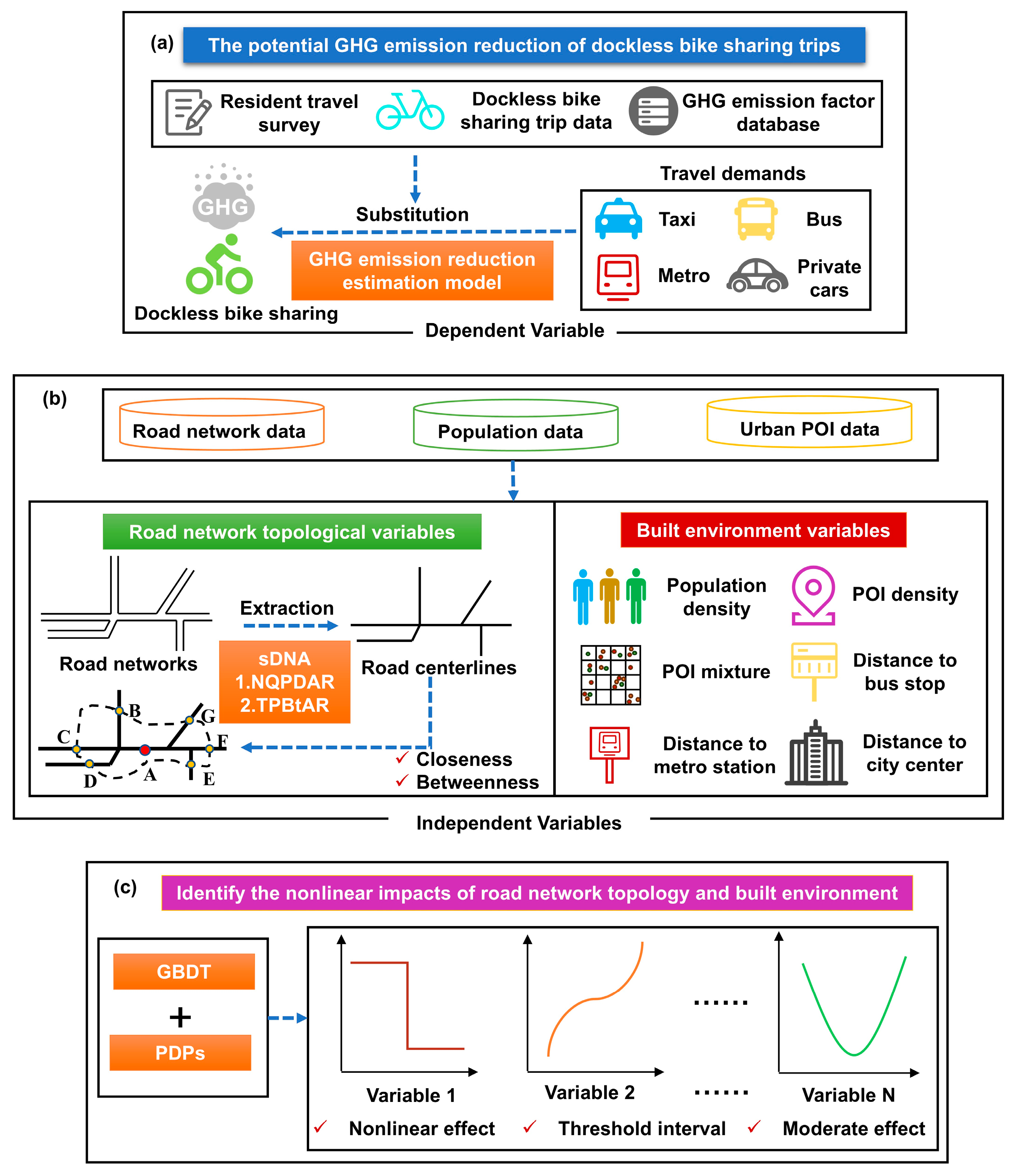
3.1. Research Framework

To explore the complex nonlinear impact mechanism of road network topology and built environment on the potential GHG emission reduction of DBS trips, we designed the research framework of this study based on multisource datasets (Figure 1). First, the potential GHG emission reduction of DBS trips was measured by the change in GHG emissions according to the potential travel mode substitution of DBS trips. The dependent variable of the research framework is the potential GHG emission reduction of DBS trips. Second, we used a spatial design network analysis (sDNA) to quantify the road network topological attributes of the study area under an optimal research scale. Moreover, we extracted several built environment indicators that prominently affect the usage of DBS from different raw datasets. Road network topological variables and built environment variables are the independent variables of the research framework. Third, a gradient boosting decision tree (GBDT) algorithm and partial dependence plots (PDPs) were employed to examine the nonlinear effects and threshold intervals of road network topology indicators and built environment elements on the potential GHG emission reduction of DBS trips. In addition, we examined how road network topology moderates the impacts of built environment elements on predicting the potential GHG emission reduction of DBS trips.

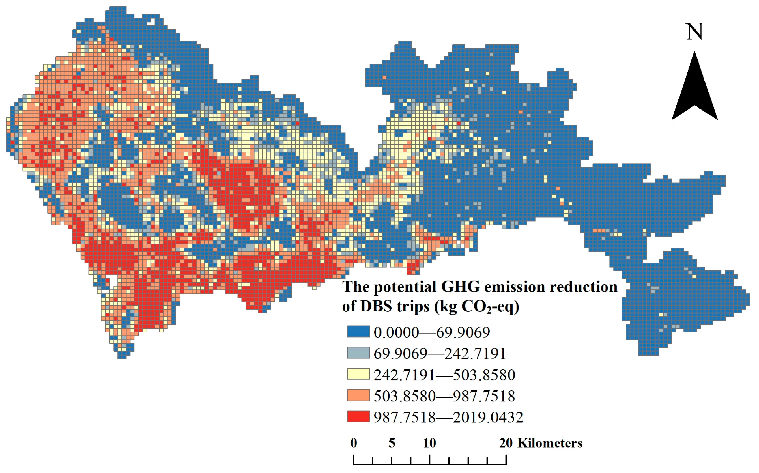
3.2. Dependent Variable

The GHG emission reduction benefits of bike sharing are often estimated by the GHG emissions of the travel modes which replace bike-sharing trips [2,10,11,39]. Existing studies often assume that all travel demands of bike sharing can be met by car travel in urban areas. However, public transport, cars, and other motorized travel modes may replace the corresponding travel volume if bike sharing is unavailable in the real world [10,26]. Moreover, travelers with a cycling distance less than 1 km are more likely to choose walking rather than motorized travel modes [10,39]. In addition, the “bottom-up” approach has been widely used to calculate the GHG emissions of the motorized travel modes in previous studies [46]. The workflow of the “bottom-up” approach begins with collecting and analyzing the underlying activity data, including travel modes, travel distance, and emission factors. This approach estimates the GHG emissions of urban transportation systems based on the gradual aggregation of these data. Therefore, we introduced an estimation model to evaluate the potential GHG emission reduction of DBS trips based on the “bottom-up” approach and motorized travel mode replacement. This estimation model considers the total distances of all DBS trips in the study area and their replacement of motorized travel modes. The detailed description is illustrated as follows: (1) Due to walking not producing GHG emissions and some motorized travel modes (e.g., motorcycle) account for a relatively small proportion of urban transportation [39], only four motorized travel modes (bus, metro, taxi, and car) are considered in the estimation model. (2) The potential GHG emission reduction of DBS trips is represented by the GHG emissions of the alternative motorized travel modes that would result from replacing all the demand for DBS trips within a distance of more than 1 km. This replacement applies to the entire demand for DBS trips in the study area and does not mean that each DBS order can be replaced with an alternative travel mode. (3) The GHG emission factors are determined by the average emission coefficient of each travel mode at the macrolevel. Accordingly, we employ the motorized split rate data of the study area to reflect the travel mode replacement of DBS trips from a macroperspective. Furthermore, this study does not consider the differences of individual trips and the impact of emergencies or major events on GHG emissions within urban transport systems. The potential GHG emission reduction of DBS trips in the study area can be denoted as Equation (1):

$$PE{R}_{GHG}={\displaystyle \sum _i{\displaystyle \sum _j{D}_i}\times M_j\times E{F}_j}$$

(1)

where $PE{R}_{GHG}$ represents the potential GHG emission reduction of DBS trips in the study area; $D_i$ denotes the travel distance (km) of the $i$th DBS order in the study area; $M_j$ is the split rate of the $j$th potential substitution travel mode in the study area; and $E{F}_j$ is the average GHG emission coefficient (kg CO₂-eq/pkm) of the $j$th travel mode during its operation phase.

3.3. Independent Variables

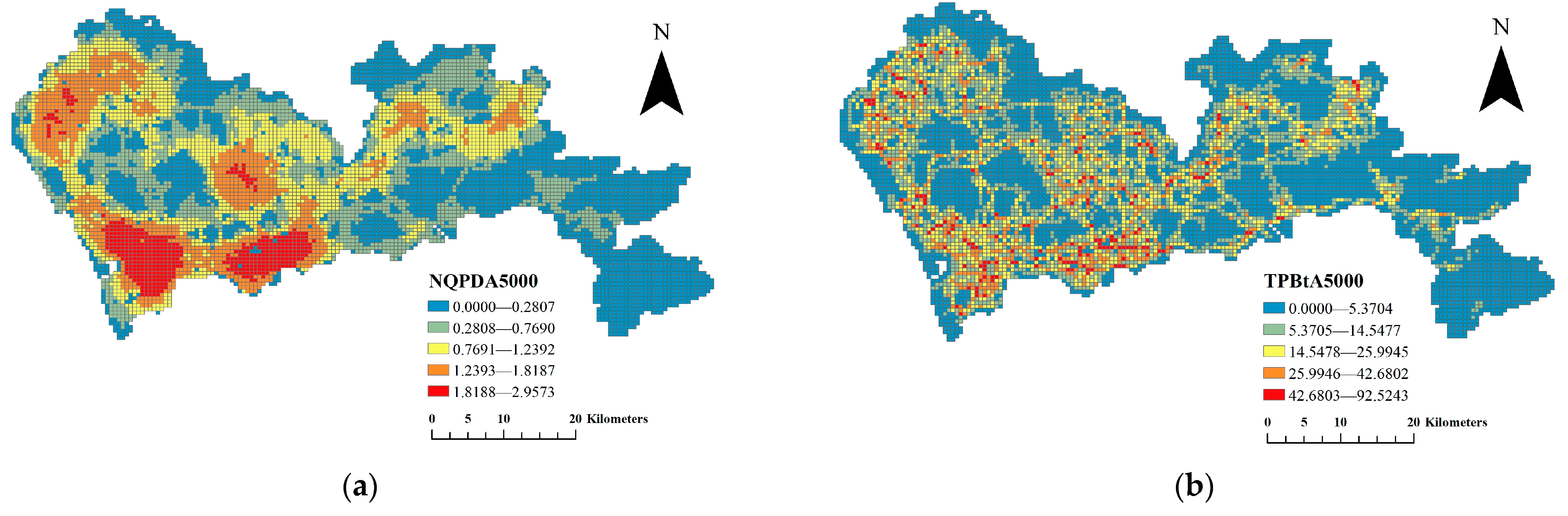
3.3.1. Road Network Topological Variable Measurement

sDNA is a sophisticated three-dimensional spatial network analysis approach, which can be applied to examine the associations between various spatial networks and transport systems. The measured output and parameters from sDNA provide evidence for the design of better networks in urban built environments. Specially, sDNA is particularly suitable for modeling sustainable transport systems. Therefore, this paper quantifies the road network topological attributes of the study area from the perspective of sDNA. In sDNA, closeness and betweenness have been usually selected by previous studies to explore the multiscale network laws [68,69], which are introduced in the following.

1.

Closeness

Closeness is employed to measure the accessibility of street networks in the study area and their ability to attract traffic flows. This topological attribute represents the relative difficulty of moving from one street link to other street links within the given road networks under different search radii. The street links with a higher closeness usually have better accessibility and make it easier for cyclists to arrive at their potential destinations [69]. This phenomenon is likely to promote the emergence of DBS orders near these street links. Network quantity penalized by distance (NQPD) is utilized to quantify closeness in sDNA [70]. Given that cyclists are inclined to follow angular geodesics, our study employs NQPD in radius angular (NQPDA) to quantify closeness, which is calculated by Equation (2):

$$NQPDAR\left(x\right)={\displaystyle \sum _{y\in R_x}\frac{w\left(y\right)p\left(y\right)}{d_A\left(x,y\right)}}$$

(2)

where $NQPDAR\left(x\right)$ represents the closeness of street link $x$ in the defined network radius $R$; $p\left(y\right)$ denotes the proportion of street link $y$ in the network radius $R$, whose value ranges from 0 to 1 in continuous space analysis and equals 0 or 1 in discrete space analysis; $R_x$ is the link set in the network radius $R$ of street link $x$; and $d_A\left(x,y\right)$ denotes the shortest angular geodesic distance from street link $x$ to $y$.

2.

Betweenness

Betweenness is employed to identify the probability of the street links that can be passed by the traffic flows in the study area. This topological attribute represents the traffic diversion capacity and passing capacity of the street networks under different search radii. In fact, the passing capacity of various traffic flows (including bikes) is often better within road networks which have a higher value of betweenness [69]. An advanced form of betweenness, namely, two phase betweenness (TPBt), is put forth to quantify betweenness in sDNA [70]. TPBt can identify and assess the potential for competition among all of the destinations within the given street networks. Given that cyclists are inclined to follow angular geodesics, our study employs TPBt angular (TPBtA) to quantify betweenness, which is calculated by Equation (3):

$$TPBtAR\left(x\right)={\displaystyle \sum _{y\in N}{\displaystyle \sum _{z\in R_{\mathrm{y}}}OD\left(y,z,x\right)}}{\displaystyle \frac{w\left(z\right)p\left(z\right)}{tw\left(y\right)}}$$

(3)

where $TPBtAR\left(x\right)$ denotes the betweenness of street link $x$ in the defined network radius $R$; $R_y$ represents the link set in the network radius $R$ of street link $y$; $w\left(z\right)$ denotes the weight of street link $z$; $N$ is the street link set in the study area; $p\left(z\right)$ represents the proportion of street link $z$ in the network radius $R$; and $tw\left(y\right)$ is the total weight of the street link set within the radius $R$ of street link $y$. $OD\left(y,z,x\right)$ represents the shortest angular geodesic route between link $y$ and link $z$ traversing link $x$ under the given network radius $R$, which is calculated by Equation (4):

$$OD\left(y,z,x\right)=\left\{\begin{array}{l}1,ifxisonthegeodesicfromytoz\\ {\displaystyle \frac{1}{2}},ifx=y\ne z\\ {\displaystyle \frac{1}{2}},ifx=z\ne y\\ {\displaystyle \frac{1}{3}},ifx=y=z\\ 0,otherwise\end{array}\right.$$

(4)

3.3.2. Built Environment Variable Selection

Urban built environment systems restrict the usage of shared bikes and residents’ travel behavior. Compared with docked bike sharing, the users of DBS are more susceptible to the impacts of built environments. Referring to previous studies [1,8,13,14,15,16,17,18,19,20,21,22,23,25,27,28,29,30,31,52,53,54,55,56,57,59,60,61], we selected 18 built environment variables that are closely associated with the utilization of DBS and its potential GHG emission reduction benefits, involving population, land use, transport accessibility, and regional location. Specifically, built environment variables include population density, restaurant density, life service density, commercial residence density, government organization density, enterprise density, education facility density, hotel facility density, sport facility density, medical service density, shopping density, tourist attraction density, POI mix entropy, bus stop density, metro station density, distance to the nearest bus stop, distance to the nearest metro station, and distance to the nearest city center. In addition, road density, intersection density, bike lanes, and bike stations are excluded in the built environment variables of this study. This is because road density and intersection density influence the topological attributes of road networks directly, which may lead to a deviation in the research conclusions. Moreover, the impacts of bike lane variables and bike station variables on the use of DBS are often insignificant in actual traffic circumstances.

3.4. Research Model and Main Algorithms

3.4.1. Gradient Boosting Decision Tree (GBDT) Algorithm

GBDT is utilized in this paper to investigate the nonlinear impact mechanism of urban road network topology and built environment on the potential GHG emission reduction of DBS trips. GBDT is a machine learning algorithm that does not make any initial assumptions about the model. By adjusting the weight of predictor variables through staged learning data, GBDT is suitable for explaining potential nonlinear relationships between different variables, and the model prediction results have a high accuracy [71,72,73,74,75,76]. At the same time, GBDT can effectively manage the issue of multicollinearity among variables and can account for missing values of independent variables [77]. In addition, GBDT is suitable for handling larger sample sizes and demonstrates strong adaptability in addressing traffic issues, particularly those that necessitate the division of study zones. GBDT has been extensively utilized in examining nonlinear relationships in urban transportation and other domains [76,78,79]. Some scholars have also applied this algorithm to the research of travel-related CO₂ emissions [80]. For this study, using GBDT has the following advantages. First, GBDT can be used to analyze the impact thresholds, effective ranges, and relative importance of road network topological indicators and built environment variables on the potential GHG emission reduction of DBS trips. Second, this study can utilize the GBDT algorithm to analyze the interaction effects between each road network topological indicator and each built environment variable on the potential GHG emission reduction of DBS trips. Equation (5) presents the mathematical form of the GBDT algorithm, which estimates the function $F(x)$ as an additive expansion of the basis function $h\left(x;{\theta }_j\right)$.

$$F\left(x\right)={\displaystyle \sum _{j=1}^m{f}_j\left(x\right)}={\displaystyle \sum _{j=1}^m{\alpha }_{j}h\left(x;{\theta }_j\right)}$$

(5)

where $x$ is a set of explanatory variables like road network topological indicators and build environment elements in this study; $F(x)$ represents the potential GHG emission reduction of DBS trips, which is the dependent variable in this study; ${\theta }_j$ denotes the mean of the split positions and terminal nodes of an individual decision tree $h\left(x;{\theta }_j\right)$; and ${\alpha }_j$ is the weight of $h\left(x;{\theta }_j\right)$, which is estimated by minimizing the loss function $L\left(y,F\left(x\right)\right)={\left(y-F\left(x\right)\right)}^2$. The optimization iterative procedure of the GBDT method is summarized in the following.

First, the initial function is set by Equation (6):

$$f_0\left(x\right)=\arg \underset{\alpha }{\min }{\displaystyle \sum _{i=1}^{n}L\left(y_i,\alpha \right)}$$

(6)

Second, for iteration rounds from $j=1$ to $m$, the negative gradient $r_{ij}$ of data sample $i$ $(i=1,2,3,\cdots ,n)$ is computed by Equation (7):

$$r_{ij}=-{\left[{\displaystyle \frac{\partial L\left(y_i,f\left(x_i\right)\right)}{\partial f\left(x_i\right)}}\right]}_{f\left(x\right)=f_{j-1}\left(x\right)}$$

(7)

Third, a regression tree $h\left(x;{\theta }_j\right)$ is fitted to the target $r_{ij}$, and the optimal gradient descent step length can thus be estimated in Equation (8):

$${\alpha }_j=\arg \underset{\alpha }{\min }{\displaystyle \sum _{i=1}^{n}L\left(y_i,F_{j-1}\left(x_i\right)+{\alpha }_{j}h\left(x_i;{\theta }_j\right)\right)}$$

(8)

The fourth step is to update the model based on Equations (7) and (8) as follows:

$$f_j\left(x\right)=f_{j-1}\left(x\right)+{\alpha }_{j}h\left(x;{\theta }_j\right)$$

(9)

The last step is to output the results of the final model as Equation (10):

$$F\left(x\right)={\displaystyle \sum _{j=1}^m{f}_j}\left(x\right)$$

(10)

To moderate the overfitting problem, a learning rate $\xi (0<\xi <1)$ is introduced to scale the contribution of each tree model. Thus, the final model can be rewritten as Equation (11):

$$f_j\left(x\right)=f_{j-1}\left(x\right)+\xi {\alpha }_{j}h\left(x;{\theta }_j\right)$$

(11)

The GBDT method provides an approach to capture the potential of reducing prediction errors according to the final model, which represents the relative importance of different independent variables. The square importance of an independent variable $x_i$ can be defined as Equations (12) and (13):

$$I_{x_i}^2={\displaystyle \frac{1}{m}}{\displaystyle \sum _{j=1}^m{I}_{x_i}^2\left(T_j\right)}$$

(12)

$$I_{x_i}^2\left(T_j\right)={\displaystyle \sum _{k=1}^h{d}_k}$$

(13)

where $I_{x_i}$ is the relative importance of independent variable $x_i$; $I_{x_i}\left(T_j\right)$ denotes the relative importance of independent variable $x_i$ when a decision tree is added to the model; $d_k$ is the corresponding improvement of squared errors if setting variable $x_i$ as the $j$th split node for each tree $T$; and $k$ represents the number of terminal nodes.

3.4.2. Partial Dependence Plots (PDPs)

The GBDT approach can depict the associations between the predicted outcome and the independent variable (usually, one or two) by producing PDPs when the other independent variables are controlled. This feature enables this study to visualize the nonlinear associations between different independent variables and the potential GHG emission reduction of DBS trips. Moreover, PDPs can be used to evaluate the interaction effects between road network topological variables and built environment variables. The partial dependence of $f_s$ on $x_s$ can be defined as Equation (14):

$$f_s\left(x_s\right)=E_{x_c}\left[f\left(x_s,x_c\right)\right]$$

(14)

where $x_c$ are the other control variables; and $E_{x_c}\left[f\left(x_s,x_c\right)\right]$ represents the marginal expectation value of $f\left(x_s,x_c\right)$. Specially, $f\left(x_s,x_c\right)$ can be calculated by the mean value of the training dataset as Equation (15):

$${\overline{f}}_s\left(x_s\right)={\displaystyle \frac{1}{n}}{\displaystyle \sum _{i=1}^n\left[f\left(x_s,x_c\right)\right]}$$

(15)

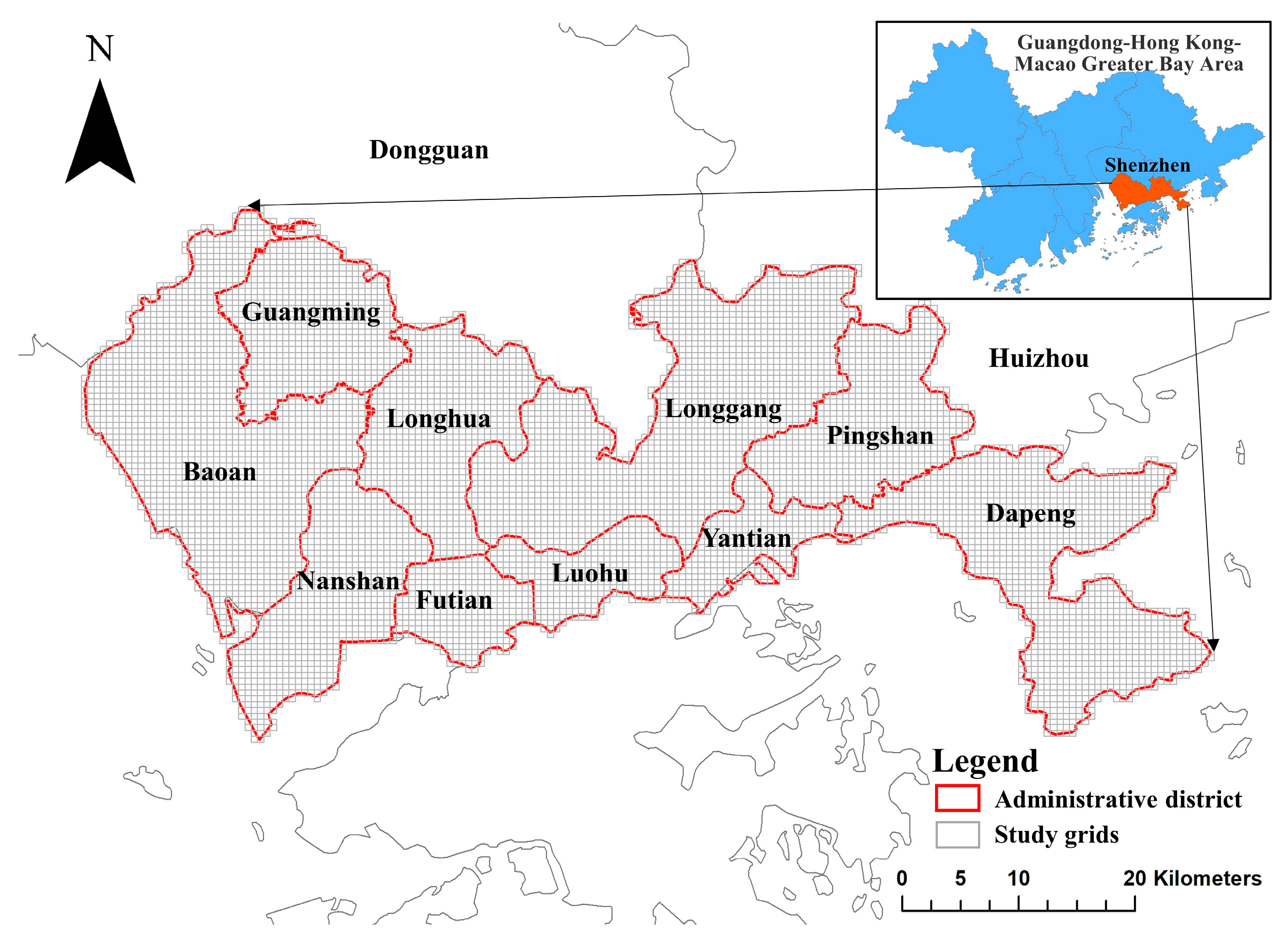
4. Study Area and Data Processing

4.1. Study Area

Shenzhen is one of the four economically developed first-tier cities in China and the central hub of the Guangdong–Hong Kong–Macau Greater Bay Area. In 2016, a DBS operation mode based on the Internet was introduced to Shenzhen. At present, Shenzhen has developed a well-established DBS system. Moreover, Shenzhen shares similar characteristics with many other cities in China in terms of planning and operating strategies for DBS. Therefore, we selected the administrative district of Shenzhen as the study area (Figure 2). According to previous studies [79,81], grid cells of 500 m × 500 m were determined as the units of analysis in this study. After removing grids without DBS trips, we attained 4260 grids for further analysis.

4.2. Data Sources and Processing

Three datasets, DBS order data, traffic GHG emission factor data, and the split rate data of various transport modes, were used to compute the dependent variable. Another three datasets, road network data, population data, and urban point of interest (POI) data, were applied to compute the independent variables.

4.2.1. DBS Order Data

The DBS order data were collected from the Shenzhen data open platform (https://opendata.sz.gov.cn/, accessed on 5 June 2022). The sample dataset used by this study spans the period from February 1 to February 14 in 2021, covering 14 days. The fields of data records contain bike ID, company ID, start time, end time, start longitude, start latitude, end longitude, and end latitude. According to the longitude and latitude information of origins and destinations, we computed the distance and the duration of each DBS trip. We removed the DBS trips with a distance less than 100 m or a duration less than 60 s [29,39]. Moreover, the trips with origins or destinations outside the study area were also deleted. In addition, we filtered out the invalid data and the data records with errors. After the above data preprocessing, 13,726,046 data records were included in this study.

4.2.2. Traffic GHG Emission Factor Data

The GHG emission coefficients of various urban travel modes in Equation (1) are sourced from the China products carbon footprint factors database (http://lca.cityghg.com/, accessed on 16 May 2022). In the database, the average GHG emission coefficient of buses is 0.01 kg CO₂-eq/pkm, the average GHG emission coefficient of metros is 0.015 kg CO₂-eq/pkm, the average GHG emission coefficient of taxis is 0.03 kg CO₂-eq/pkm, and the average GHG emission coefficient of cars is 0.034 kg CO₂-eq/pkm (

Table 1. GHG emission coefficients of various travel modes.

	Bus	Metro	Taxi	Car
GHG emission coefficient (kg CO2-eq/pkm)	0.01	0.015	0.03	0.034

).

4.2.3. Split Rate Data of Different Transport Modes

The split rate data of various transport modes were obtained from the Seventh Resident Travel Survey of Shenzhen. According to the survey results, in Shenzhen, the proportion of travel in private cars is 53%, the proportion of travel by bus is 18%, the proportion of travel by metro is 20%, the proportion of travel in taxis is 5%, and other modes account for 3%. Based on the above three datasets and Equation (1), we calculated the potential GHG emission reduction of DBS trips in each study grid. Figure 3 shows the spatial distribution of the potential GHG emission reduction of DBS trips in Shenzhen.

4.2.4. Road Network Data

The road network data were obtained from an open geographic map database, OpenStreetMap (https://www.openstreetmap.org/, accessed on 20 March 2021). Some roads and transportation facilities were removed as follows: (1) restricted roads that are located in an enclosed area such as a community, school, park, etc.; (2) roads that are impassable or restricted for bikes; (3) pedestrian road-supporting facilities such as steps, overpasses, etc. In addition, road centerline vector data are necessary for sDNA analysis. However, the road network data from OpenStreetMap is multiline data (one road is represented by multiple lines). Therefore, we extracted the road centerline vector data from simplified road network data through GIS tools including Buffer, Reclass, and ArcScan. On this basis, we calculated the closeness and betweenness within the various search radii of the road networks in each grid according to Equations (2)–(4). The search radii include 800 m, 1600 m, 2500 m, 3000 m, 5000 m, 8000 m, 10,000 m, 15,000 m, and 20,000 m, which reflect the topological features of the road networks under different research scales. In addition, these search radii can cover nearly all the DBS orders with different trip distances and trip durations. We finally selected the search radius of 5000 m, which corresponds to the GBDT model with the optimal goodness of fit. Therefore, NQPDA5000 and TPBtA5000 were used to represent the road network topological variables in this study (Figure 4).

4.2.5. Population Data

The population density data of Shenzhen is sourced from the WorldPop website (https://www.worldpop.org, accessed on 15 January 2023). According to the data from the Seventh Population Census of Shenzhen, we further amended the population data of each grid in the study area. Based on the above grid population data, we used the method proposed by Li and Liu (2018) [82] to extract eight urban centers of Shenzhen (as shown in Figure 5). Since regional location is crucial to DBS trips, the distance of each grid centroid to the closest city center centroid was computed to interpret the impacts of its location in the study area.

4.2.6. Urban POI Data

The urban POI data were acquired from Gaode Map (https://lbs.amap.com/, accessed on 5 March 2021). This dataset contains 12 types of POIs, including transport-related, restaurant, life service, sports, enterprises, hospital-related, commercial residence, government organization, education-related, shopping, hotel-related, and tourist-related. This dataset enables us to estimate the land use in the grids by measuring the density of each type of POI [29,30]. Moreover, we computed the distance of each grid centroid to its nearest bus stop/metro station. Furthermore, we measured the POI mix entropy in each grid to quantify the land use mixture of different research regions, which is formulated as Equation (16):

$$PM{E}_i=-{\displaystyle \sum _{i=1}^n{P}_{ik}\times \log }{P}_{ik}$$

(16)

where $PM{E}_i$ denotes the POI mix entropy of the study grid $i$; and $P_{ik}$ represents the ratio of the $k$th POI in the study grid $i$.

Table 2. Descriptive statistics of the dependent variable and independent variables.

Variables	Description	Data Sources	Min	Max	Mean	St. Dev
The potential GHG emission reduction of DBS trips	Transport-related GHG emission reduction caused by DBS in each study grid, kgCO2-eq	(1) DBS data of the Shenzhen data open platform (2) China products carbon footprint factors database (3) The Seventh Resident Travel Survey of Shenzhen	0	2019.04	97.29	192.13
NQPDA5000	The closeness within the network radius R (R = 5000 m) of each study grid, scale	(4) OpenStreetMap geographic map database	0	2.96	1.06	0.63
TPBtA5000	The betweenness within the network radius R (R = 5000 m) of each study grid, scale		0	92.52	14.20	13.04
Population density	Population per km2 in each study grid, persons/km2	(5) WorldPop population data website	0	187,516.4	14,205.8	16,343.52
Restaurant density	Number of restaurants per km2 in each study grid, count/km2	(6) The urban POI data from Gaode Map	0	1084	64.08	111.69
Life service density	Number of life services per km2 in each study grid, count/km2		0	612	34.16	64.26
Commercial residence density	Number of commercial residences per km2 in each study grid, count/km2		0	864	23.52	36.81
Government organization density	Number of government organizations per km2 in each study grid, count/km2		0	308	12.79	26.49
Enterprise density	Number of enterprises per km2 in each study grid, count/km2		0	1824	116.63	178.29
Education facility density	Number of education facilities per km2 in each study grid, count/km2		0	584	23.32	43.55
Hotel facility density	Number of hotel facilities per km2 in each study grid, count/km2		0	612	10.03	25.74
Sport facility density	Number of sport facilities per km2 in each study grid, count/km2		0	300	14.51	25.80
Medical service density	Number of medical services per km2 in each study grid, count/km2		0	268	17.43	31.60
Shopping density	Number of shopping services per km2 in each study grid, count/km2		0	88	4.37	8.21
Tourist attraction density	Number of tourist attractions per km2 in each study grid, count/km2		0	152	1.83	5.80
Land use mixture	Mix entropy of various types of POIs, calculated by Equation (16), scale		0	2.41	1.13	0.80
Bus stop density	Number of bus stops per km2 in each study grid, count/km2		0	412	33.38	49.47
Distance to the nearest bus stop	Distance from the centroid of each study grid to the nearest bus stop, m		2.67	3182.95	357.15	349.60
Metro station density	Number of metro stations per km2 in each study grid, count/km2		0	12	0.25	1.09
Distance to the nearest metro station	Distance from the centroid of each study grid to the nearest metro station, m		15.93	31,163.89	2255.06	2670.99
Distance to the nearest city center	Distance from the centroid of each study grid to the nearest city center, m		43.94	41,058.5	6063.92	3938.47

presents the descriptive statistics of the dependent variable and independent variables used in this study.

5. Results and Discussion

5.1. Model Regulation

To avoid potential overfitting and obtain model results with robustness, this study applied a five-fold cross-validation to train the GBDT model. According to previous studies [77,78,83], we set the learning rate at 0.001. Using the “HyperOpt” package in the Python language, two other crucial parameters were determined: the number of trees and tree complexity. Via this powerful Python library, we finally set the maximum number of trees at 10,000 and chose a tree complexity of 10. The pseudo R² of the best model is 0.346.

5.2. Relative Importance of Independent Variables

Table 3. Relative importance of independent variables in predicting the potential GHG emission reduction of DBS trips.

Categories	Variables	Ranking	Relative Importance (%)	Sum (%)
Road network topological attributes	NQPDA5000	1	31.32	37.81
	TPBtA5000	5	6.49
Population	Population density	3	8.95	8.95
Land use	Restaurant density	12	2.71	28.69
	Life service density	16	1.72
	Commercial residence density	9	3.01
	Government Organization density	13	2.53
	Enterprises density	7	3.98
	Education facility density	11	2.80
	Hotel facility density	17	1.53
	Sport facility density	14	2.41
	Medical service density	15	1.77
	Shopping density	19	1.12
	Tourist attraction density	18	1.22
	POI mix entropy	8	3.89
Transport accessibility	Bus stop density	10	2.99	17.17
	Distance to the nearest bus stop	6	4.91
	Metro station density	20	0.13
	Distance to the nearest metro station	2	9.14
Regional location	Distance to the nearest city center	4	7.38	7.38

illustrates the relative importance of all the independent variables in predicting the potential GHG emission reduction of DBS trips and their contribution rankings. Both road network topological variables collectively contribute to 37.81% of the prediction, which shows their important role in reducing GHG emissions and guiding the development of DBS in Shenzhen. This partly corresponds to a study illustrating the important role of street patterns in influencing bike-sharing usage [29]. In particular, the relative importance of NQPDA5000 is 31.32%, while the contribution of TPBtA5000 accounts for 6.49%, ranking first and fifth. This indicates that closeness has a stronger predictive power in predicting the potential GHG emission reduction of DBS trips compared to betweenness. Among all the independent variable categories, the contribution of land use attributes is second only to road network topology, with a relative importance of 28.69%. Specifically, the contributions of the 12 land use variables range from 1% to 4%. The relative importance of commercial residence density, enterprise density, and POI mix entropy exceeds 3%. This finding suggests that, compared to other land use variables, a high density of employment and housing plays an indispensable role in predicting the potential GHG emission reduction of DBS trips. Also, all land use variables have at least a relative importance of 1% for prediction. Transit-related variables collectively explain 17.17% of the variation in predicting the dependent variable, ranking third among all variable categories. Overall, bus stop density contributes more to predicting the potential GHG emission reduction of DBS trips than metro station density. However, the relative importance of distance to the nearest metro station is greater than that of distance to the nearest bus stop, consistent with previous studies [1,30,54]. This phenomenon is probably due to bus stops being more easily available, whereas metro stations can provide more ridership. In addition, the contribution of the distance to the nearest station to the prediction is much higher than station density, whether it is bus or metro. The relative importance of population density and distance to the nearest city center account for 8.95% and 7.38%, respectively, ranking third and fourth.

5.3. Nonlinear Effects of Independent Variables

By visualizing the marginal effects of road network topological variables and built environment variables with PDPs, we further investigated the effective ranges and threshold effects of each independent variable on predicting the potential GHG emission reduction of DBS trips. As is shown in Figure 6, we plotted the PDPs of the eight most important variables tested in the GBDT model.

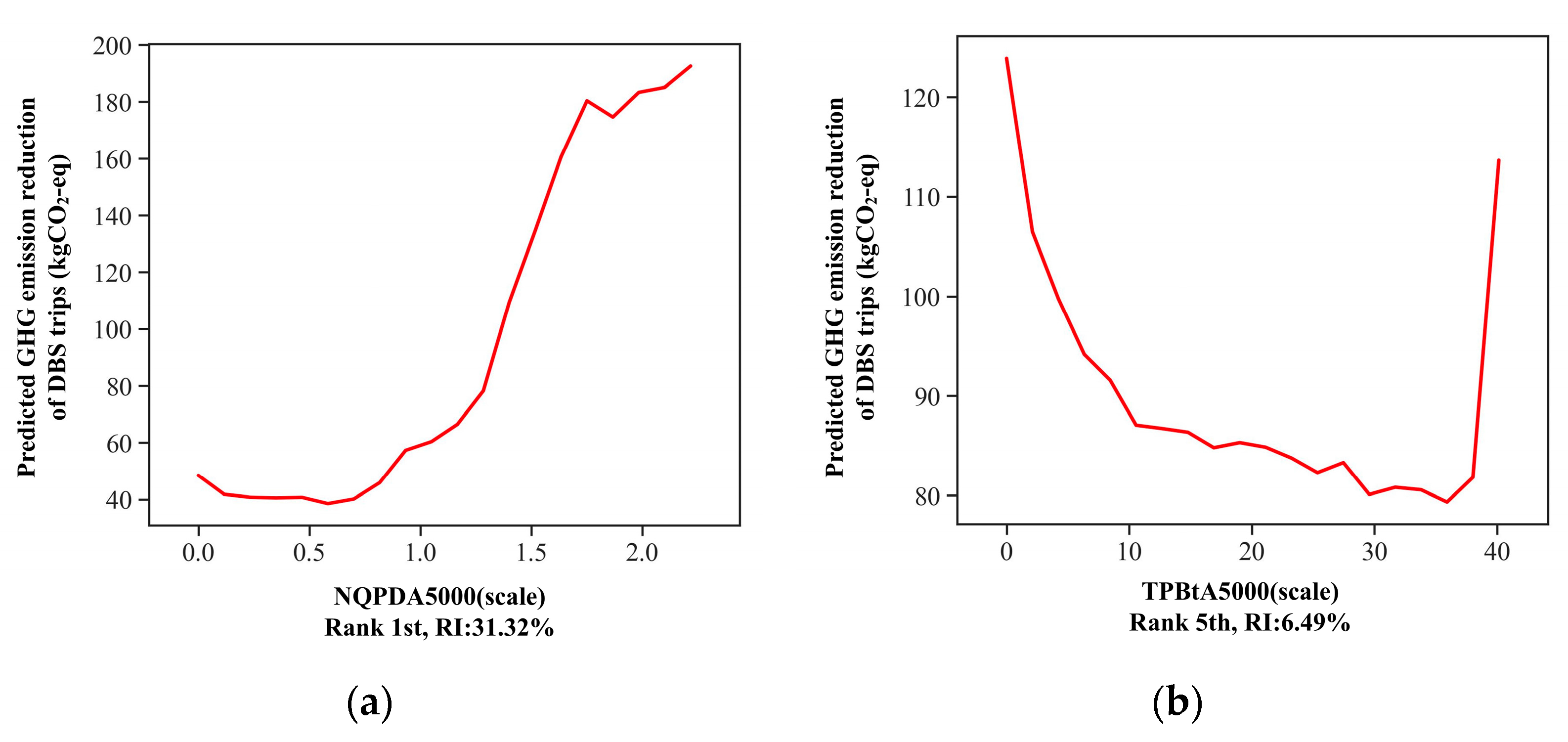
5.3.1. Road Network Topological Variables

Figure 6a illustrates the nonlinear impacts and threshold intervals of NQPDA5000 when predicting the potential GHG emission reduction of DBS trips. As NQPDA5000 increases from 0.6 to 1.75, the predicted value rapidly increases from 39 to 180 kgCO₂-eq. In this interval, NQPDA5000 is positively related to the predicted value. When the value of NQPDA5000 is within the ranges of 0 to 0.6 and 1.75 to 1.87, the predicted value decreases, but the change is relatively small (the former is about 10 kgCO₂-eq, the latter is about 6 kgCO₂-eq). When the value of NQPDA5000 exceeds 1.87, the predicted value increase slightly. Overall, there is a positive correlation between NQPDA5000 and the predicted value. The reason is that as the value of closeness increases, the accessibility of the road networks gradually improves. Previous studies have proven that road networks with better accessibility can promote bike usage [41,54]. Moreover, multitudinous commercial centers, recreation places, office buildings, catering, and other facilities are located in the adjacent areas where the closeness of road networks is high. These factors stimulate bike-sharing travel and corresponding GHG emission reduction. In addition, 1.75 may be a critical value for the effective range of NQPDA5000. The impact of NQPDA5000 becomes trivial when it exceeds 1.75. Furthermore, whether in the design or construction stages, the closeness of road networks cannot increase indefinitely. In Shenzhen, government managers should focus on the changes in DBS’s GHG emission reduction with NQPDA5000 ranging from 0.6 to 1.75. Correspondingly, planners should also refer to the value of closeness in Shenzhen when designing bike lanes and road networks. Meanwhile, bike-sharing enterprises should appropriately expand the service scope of shared bikes in areas where NQPDA5000 is less than 0.6. For areas where NQPDA5000 exceeds 1.75, the number of shared bikes should be increased.

As shown in Figure 6b, the nonlinear association between TPBtA5000 and the potential GHG emission reduction of DBS trips presents a U-shaped relationship. As TPBtA5000 increases from 0 to 10.5, the predicted value of DBS decreases rapidly. Subsequently, it becomes flat with a slight decrease when TPBtA5000 increases from 10.5 to 36. By contrast, when TPBtA5000 exceeds 36, the predicted value increase rapidly again. Overall, when the value of TPBtA5000 is larger or smaller, nearby DBS orders often have relatively high GHG emission reduction potential. For these areas, the number of shared bikes should be increased. In fact, urban expressways, arterial roads, or the roads which locate in urban core areas often have a higher value of betweenness. In general, the closeness of the road networks in such areas is also relatively high. Furthermore, the street links which have a lower betweenness are mainly situated in the suburban areas of the urban periphery or the branch roads connected to the main roads of the urban core areas. For the former, travelers frequently need to ride longer distances to complete the “first mile” and “last mile” of their trips. For the latter, the branch roads bear the microcirculation function of the urban transport system and are close to the main roads, transport stations, and commercial districts. Nearby areas have the potential to form more DBS orders.

5.3.2. Built Environment Variables

The relationship between the potential GHG emission reduction of DBS trips and the distance to the nearest metro station shows a V-shaped curve, and the turning point is about 2500 m (Figure 6c). When distance to the nearest metro station increases from 0 to 1000 m, the predicted value is limited at a higher level, and its change is trivial. As the distance to the nearest metro station increases from 1000 to 2500 m, the predicted value sharply decreases by about 33 kgCO₂-eq. For the previous interval, the number of shared bikes should be increased to maximize GHG emission reduction potential. For the latter interval, bike-sharing enterprises should appropriately expand the service scope of shared bikes. When distance to the nearest metro station exceeds 2500 m, the predicted value increases again and gradually levels off. In this interval, bike-sharing enterprises should further adjust their electronic fence and rebalance scheme to enhance the potential GHG emission reduction of DBS trips.

As shown in Figure 6d, the relationship between the potential GHG emission reduction of DBS trips and the distance to the nearest bus stop shows a V-shaped curve, and the turning point is about 320 m. As the distance to the nearest bus stop increases from 0 to 320 m, the predicted value decreases by about 4 kgCO₂-eq. Some travelers whose destinations are bus stops tend to walk within this distance range. The trip distance of bike-sharing users who complete their “last mile” between bus stops and their residences is usually relatively short. To some extent, this inhibits the potential GHG emission reduction of DBS trips. Bike-sharing enterprises should appropriately expand the service scope of shared bikes within this distance interval. When distance to the nearest bus stop increases from 320 to 770 m, the predicted value rapidly increases from 84 to 98.7 kgCO₂-eq. In this range, bike-sharing enterprises should further adjust their electronic fence and rebalance scheme to increase the potential GHG emission reduction of DBS trips. The impact of the distance to the nearest bus stop becomes trivial when it exceeds 770 m. In this interval, the number of shared bikes should be increased to maximize GHG emission reduction potential. It is worth noting that compared to bus stops, the distance critical value for metro stations to have a positive impact on the potential GHG emission reduction of DBS trips is larger. This phenomenon is reasonable because the service scope of metro stations and their ability to attract DBS trips are significantly higher than that of bus stops [28,84].

The nonlinear association between the potential GHG emission reduction of DBS trips and population density presents an inversely N-shaped relationship (Figure 6e). This finding is not consistent with other empirical studies, which implies that population density is positively associated with bike-sharing usage [21,28]. As population density increases from 0 to 5000 persons per km², the predicted value decreases for unknown reasons. When population density ranges from 5000 to 37,500 persons per km², the predicted value fluctuates but shows a trend of continuous growth. In contrast, when population density exceeds 37,500 persons per km², the predicted value decreases again. This may be due to excessive population density leading to a decrease in cycling comfort within areas. Therefore, some bike-sharing cyclists choose other transport modes or use shared bikes in other areas. Overall, when the population density is about 37,500 persons per km², the predicted value reaches its peak. Bike-sharing enterprises should rebalance shared bikes in areas with higher population density. By appropriately reducing the number of shared bikes in these areas during peak hours, the waste of traffic resources can be avoided.

As shown in Figure 6f, the nonlinear association between the potential GHG emission reduction of DBS trips and the distance to the nearest city center presents an inversely N-shaped relationship. When distance to the nearest city center is lower than 2000 m, it has a negative association with the predicted value. This is consistent with our understanding that the attraction of city centers for bike-sharing trips gradually diminishes as distance increases. When the distance to the nearest city center ranges from 2000 to 3000 m, it has a positive effect on the predicted value. This distance range corresponds to the optimal travel distance for bike sharing, while travelers are attracted to city centers. Travelers with trip starting points within this range will have to walk longer distances to reach city centers. Moreover, the usage of public transport and private cars may hinder their travel experiences and convenience because of issues such as traffic congestion and difficulty finding parking. Therefore, bike sharing has emerged as the optimal solution. In this distance range, the number of shared bikes should be increased to enhance GHG emission reduction potential. Notably, as the distance to the nearest city center increases from 3000 to 6800 m, the predicted value decreases drastically. When the distance to the nearest city center is 3000 m, the predicted value seems to be a local peak. In this interval, bike-sharing enterprises should appropriately decrease the number of shared bikes. Furthermore, when distance to the nearest city center exceeds 6800 m, the association between it and the potential GHG emission reduction of DBS trips presents an inversely U-shaped relationship. In this range, the change in the predicted value is relatively small (about 4 kgCO₂-eq). The service scope of shared bikes should be appropriately expanded within this distance interval.

The relationship between enterprise density and the potential GHG emission reduction of DBS trips shows a V-shaped curve, and the turning point is about 90 counts per km² (Figure 6g). When enterprise density increases from 0 to 90 counts per km², the predicted value rapidly decreases by about 16 kgCO₂-eq. In contrast, as enterprise density exceeds 90 counts per km², the predicted value continuously increases. There are inherent reasons for the emergence of this phenomenon. On the one hand, some areas with a lower enterprise density are located at the urban fringe and in suburbs. Public transport commuters in these areas may need to use DBS to complete the “first mile” and “last mile” of their trips. Moreover, they usually ride a long distance. On the other hand, although enterprise density in some areas is low, there are more job opportunities in the adjacent areas near them. This means that travelers in these areas can use bike sharing to complete commuting, which will enhance the probability to form more bike-sharing orders. Notably, when enterprise density ranges from 250 to 270 counts per km², the predicted value increases at the fastest rate. When enterprise density exceeds 390 counts per km², the increase rate of the predicted value ranked second. Therefore, bike-sharing operators should focus on the reasonable allocation of shared bikes and the optimization of their electronic fence in areas with an enterprise density ranging from 250 to 270 counts per km², rather than only focusing on areas with the highest enterprise density. In addition, encouraging new companies to settle in the areas corresponding to this range is also one of the options to increase the GHG emission reduction potential of bike sharing in these areas.

Figure 6h depicts that POI mix entropy has a positive association with the potential GHG emission reduction of DBS trips. This is in accordance with the current literature that has examined the relationships between land use and bike-sharing trips [31,52]. When the entropy index increases from 0 to 1.7, the predicted value fluctuates, and the largest change is only about 2.5 kgCO₂-eq. Subsequently, as the entropy index exceeds 1.7, the predicted value starts to increase. In particular, the predicted value increases with the greatest rate of rise when the entropy index exceeds 2.05. This indicates that 2.05 may be a critical value for the effective range of POI mix entropy. Bike-sharing trips and their related GHG emission reduction effect increases substantially when the entropy index exceeds this critical value. For areas with entropy values less than 1.7, the service scope of shared bikes should be appropriately expanded. Furthermore, the areas with an entropy value ranging from 1.7 to 2.05 are potential areas for increasing various service facilities and POIs. In addition, for areas with an entropy value exceeding 2.05, the number of shared bikes should be increased to enhance GHG emission reduction potential.

5.4. Interaction Effects between Road Network Topological Variables and Built Environment Variables

PDPs with two input features can help us further examine how some variables moderate the effects of the other variables in predicting the potential GHG emission reduction of DBS trips. Figure 7 presents these interaction effects between road network topological variables (NQPDA5000 and TPBtA5000) and the other six most important variables. For different built environment variables, the same road network topological variable shows similar moderating effects as follows. Overall, the impact of each variable on the potential GHG emission reduction of DBS trips increases as the value of the closeness variable increases. In contrast, when the value of the betweenness variable is too large or too small, it presents evident moderating effects on each variable. These findings correspond to the effective ranges of NQPDA5000 and TPBtA5000, as illustrated in Section 5.3. Notably, compared with betweenness, closeness has a greater moderating effect on the nonlinear associations between each variable and the potential GHG emission reduction of DBS trips. For example, the variation in the predicted GHG emission reduction of DBS trips exceeds 200 kgCO₂-eq when the input features are NQPDA5000 and population density (Figure 7(a1)). However, the variation in the predicted GHG emission reduction of DBS trips is less than 60 kgCO₂-eq when the input features are TPBtA5000 and population density (Figure 7(b1)). This indicates that closeness may have a more significant interaction effect on the other independent variables than betweenness. The reasons for this phenomenon are elucidated in the following. For one thing, due to the better performance in topological centrality and integration, the road networks with the higher closeness have become a more attractive option for bike trips and other traffic flows in adjacent areas. In the meantime, the potential for experiencing traffic congestion is more likely to occur on these road networks. Thus, to avoid excessive queues and slower vehicle speeds, some travelers prefer to adapt to bike sharing rather than a motorized travel mode. For another, the POIs with multiple service functions are often distributed in the road networks with the higher closeness, and cyclists can easily reach their potential destinations. Consequently, there is a greater probability that the DBS orders with shorter trip distances and shorter trip durations are formed in adjacent areas.

5.5. Comparison with Linear Regression

To verify the rationality of the nonlinearity assumption between independent variables and the dependent variable, we developed an ordinary least squares (OLS) model and compared it with the GBDT model.

Table 4. The results of the OLS model.

Variables	Coefficients	Relative Importance (%)	Sum (%)
NQPDA5000	130.81	33.44	37.38
TPBtA5000	−1.59	3.93
Population density	0.0016	12.66	12.66
Restaurant density	−0.12	2.38	38.40
Life service density	0.09	2.54
Commercial residence density	0.50	6.15
Government organization density	0.25	4.39
Enterprise density	−0.05	2.42
Education facility density	0.17	6.35
Hotel facility density	0.24	1.97
Sport facility density	0.85	5.04
Medical service density	−0.40	2.34
Shopping density	−0.33	1.39
Tourist attraction density	−0.03	0.37
POI mix entropy	−15.23	3.07
Bus stop density	0.21	3.28	9.26
Distance to the nearest bus stop	0.05	2.46
Metro station density	0.83	0.94
Distance to the nearest metro station	−0.0024	2.58
Distance to the nearest city center	0.0015	2.30	2.30
Sample size	4260
R-squared	0.244

shows the estimated coefficients and the relative importance of all the independent variables in the OLS model. With respect to the research topic of this study, the GBDT model has obvious advantages in a few aspects. On one hand, 34.6% of the variation in the potential GHG emission reduction of DBS trips is explained by the GBDT model. However, the R² of the OLS model is 0.244, which means that only 24.4% of the variation is explained by the same independent variables. The PDPs in the GBDT model also show these nonlinear relationships and the impact threshold of each variable. That is because GBDT does not assume any form of linear relationship between the potential GHG emission reduction of DBS trips and independent variables. In contrast, the OLS model has a limited capacity to reveal the potential nonlinear associations, and its PDPs can only illustrate the positive or negative effects of each variable. Other scholars have obtained similar results in their studies [79,83]. On the other hand, the GBDT model considers the interaction effects among the variables at different levels of the decision trees. In Section 5.4, we illustrated the interaction effects between road network topological variables and built environment variables. Usually, the OLS model and other linear regression models are unable to analyze these effects.

6. Conclusions

This study designed a research framework to identify the nonlinear impacts of road network topological attributes and built environment elements on the potential GHG emission reduction of DBS trips in Shenzhen, China. Various methods were employed in this research framework, including a GHG emission reduction estimation model, spatial design network analysis (sDNA), gradient boosting decision tree (GBDT) algorithm, and partial dependence plots (PDPs). Furthermore, we also assessed the interaction effects between road network topological variables and built environment variables. The findings contribute to the existing knowledge of bike sharing’s environmental benefits by providing empirical evidence. In addition, the insights gained from this study may be of assistance to bike-sharing system planning, bike-sharing rebalancing strategy optimization, and low-carbon travel policy formulation. The main research conclusions are summarized in the following.

First, the eight most important variables for the potential GHG emission reduction of DBS trips are NQPDA5000, distance to the nearest metro station, population density, distance to the nearest city center, TPBtA5000, distance to the nearest bus stop, enterprise density, and POI mix entropy. In particular, the total contribution of the road network topological variables ranks first among all the variables, exceeding the land use variables and transit-related variables. This result confirms the leading role of road network topological attributes in determining the potential GHG emission reduction of DBS trips. In fact, road network topological factors have often been ignored in previous studies. Therefore, it is necessary to consider road network topological variables in the future research on the environmental benefits of bike sharing and other travel modes.

Second, the nonlinear influences of road network topological variables and built environment variables are prevalent and show certain threshold intervals for the potential GHG emission reduction of DBS trips. The results show that when NQPDA5000 reaches 1.75, and the distance to the nearest metro station, population density, distance to the nearest city center, and distance to the nearest bus stop reach 1000 m, 37,500 persons per km², 3000 m, and 770 m, respectively, the potential GHG emission reduction of DBS trips in Shenzhen reaches critical values. For the sake of increasing the potential GHG emission reduction effectively, some threshold intervals suggested by our empirical findings also need to be considered. For example, NQPDA5000 should be within 0.6–1.75; the distance to the nearest metro station should be within 1000 m; the distance to the nearest city center should be within 2000–3000 m; the distance to the nearest bus stop should be within 320–770 m; enterprise density should be within 250–270 counts per km²; and the POI mix entropy should exceed 2.05. Furthermore, TPBtA5000 becomes effective when it is within 10.5 or it exceeds 36. The threshold effects of each variable inform planners and policy makers to meticulously adjust land use guidelines and built environments. In addition, bike-sharing operators can utilize this quantitative evidence to design their electronic fence and optimize their bike-rebalancing scheme.

Third, the impact of built environment attributes on the potential GHG emission reduction of DBS trips is moderated by road network topological indicators (closeness and betweenness). Specifically, the larger positive effect of each built environment variable corresponds to the higher value of the closeness. In contrast, when the value of the betweenness variable is too large or too small, the impact of each variable reaches the higher level. In comparison to betweenness, closeness moderates the effects of the built environment attributes in a significant way. These findings provide a new inspiration for future urban road network planning and design. Furthermore, it also provides more opportunities for planners to formulate a more sustainable and green transportation development blueprint. Bike-sharing operators should pay attention to the impact of road network topological attributes (especially closeness) on the environmental benefits of bike sharing. When considering the influence of road network topology, planners can also supply cyclists with a more comfortable and convenient urban built environments.

Further studies are required to address the following limitations. First, the generalizability of the effective thresholds found in Shenzhen should be further investigated. Shenzhen is one of the four first-tier megacities in China, with a high level of urbanization and a mature bike-sharing operation system. Therefore, we selected Shenzhen as a case study to examine the capability of DBS to reduce GHG emissions. However, the road networks of Shenzhen show typical cluster layout characteristics, and the research findings of such cites may be unique [78]. Future work should examine more cities with other forms of layout (such as linear layout and satellite layout). Second, existing studies have proven that the topological features of urban road networks can affect the route choice tendency of travelers, especially slow traffic participants [32,33,34]. Due to the protection of travelers’ privacy by bike-sharing operators, we are unable to contact the order users. This means that we cannot investigate the socioeconomic attributes of travelers and their views on how road network topology affects travel behavior. It is recommended that researchers further extend the results of our study from this perspective. Third, this study only evaluated the nonlinear associations between the influencing factors and the potential GHG emission reduction of bike-sharing operations. However, bike sharing still has environmental impacts from the other phases of its life cycle (e.g., bike manufacturing and bike rebalancing) [12,44,45]. We encourage researchers in related fields to comprehensively analyze and compare the life cycle GHG emission characteristics and influencing factors of bike-sharing systems. Fourth, the computing method to assess the potential GHG emission reduction of DBS trips needs to be further explored. On the one hand, the emerging modes of transportation (e.g., personal e-scooters, e-bikes) and the economic factors (e.g., bicycle loan costs, public transport fares, and fuel costs for private vehicles) should also be covered by future research. On the other hand, more precise results can be obtained if the potential travel mode replacement of each DBS trip is estimated accurately. This would be a fruitful area for further work. On this basis, planners can better understand the internal associations among the environmental footprint of bike-sharing systems, urban built environments, and socioeconomic factors. Moreover, these findings can also provide decision makers with more refined policy recommendations.

References

1. Guo, Y.Y.; He, S.Y. Built environment effects on the integration of dockless bike-sharing and the metro. Transp. Res. Part D Transp. Environ. 2020, 83, 102335. [Google Scholar] [CrossRef]
2. Diao, M.; Song, K.; Shi, S.; Zhu, Y.; Liu, B. The environmental benefits of dockless bike sharing systems for commuting trips. Transp. Res. Part D Transp. Environ. 2023, 124, 103959. [Google Scholar] [CrossRef]
3. Shaheen, S.; Chan, N. Mobility and the sharing economy: Potential to facilitate the first-and last-mile public transit connections. Built Environ. 2016, 42, 573–588. [Google Scholar] [CrossRef]
4. Liu, L.M.; Sun, L.J.; Chen, Y.Y.; Ma, X.L. Optimizing fleet size and scheduling of feeder transit services considering the influence of bike-sharing systems. J. Clean. Prod. 2019, 236, 117550. [Google Scholar] [CrossRef]
5. Cheng, Y.H.; Lin, Y.C. Expanding the effect of metro station service coverage by incorporating a public bicycle sharing system. Int. J. Sustain. Transp. 2018, 12, 241–252. [Google Scholar] [CrossRef]
6. Cao, Y.J.; Shen, D. Contribution of shared bikes to carbon dioxide emission reduction and the economy in Beijing. Sustain. Cities Soc. 2019, 51, 101749. [Google Scholar] [CrossRef]
7. Bullock, C.; Brereton, F.; Bailey, S. The economic contribution of public bike-share to the sustainability and efficient functioning of cities. Sustain. Cities Soc. 2017, 28, 76–87. [Google Scholar] [CrossRef]
8. Bi, H.; Li, A.Y.; Hua, M.Z.; Zhu, H.; Ye, Z.R. Examining the varying influences of built environment on bike-sharing commuting: Empirical evidence from Shanghai. Transp. Policy 2022, 129, 51–65. [Google Scholar] [CrossRef]
9. Zhang, Y.P.; Mi, Z.F. Environmental benefits of bike sharing: A big data-based analysis. Appl. Energy 2018, 220, 296–301. [Google Scholar] [CrossRef]
10. Saltykova, K.; Ma, X.L.; Yao, L.L.; Kong, H. Environmental impact assessment of bike-sharing considering the modal shift from public transit. Transp. Res. Part D Transp. Environ. 2022, 105, 103238. [Google Scholar] [CrossRef]
11. Li, A.Y.; Gao, K.; Zhao, P.X.; Qu, X.B.; Axhausen, K.W. High-resolution assessment of environmental benefits of dockless bike-sharing systems based on transaction data. J. Clean. Prod. 2021, 296, 126423. [Google Scholar] [CrossRef]
12. Luo, H.; Zhao, F.; Chen, W.Q.; Cai, H. Optimizing bike sharing systems from the life cycle greenhouse gas emissions perspective. Transp. Res. Part C Emerg. Technol. 2020, 117, 102705. [Google Scholar] [CrossRef]
13. Alcorn, L.G.; Jiao, J.F. Bike-Sharing Station Usage and the Surrounding Built Environments in Major Texas Cities. J. Plan. Educ. Res. 2023, 43, 122–135. [Google Scholar] [CrossRef]
14. Duran-Rodas, D.; Chaniotakis, E.; Antoniou, C. Built Environment Factors Affecting Bike Sharing Ridership: Data-Driven Approach for Multiple Cities. Transp. Res. Rec. 2019, 2673, 55–68. [Google Scholar] [CrossRef]
15. Wang, L.; Zhou, K.C.; Zhang, S.R.; Moudon, A.V.; Wang, J.F.; Zhu, Y.G.; Sun, W.Y.; Lin, J.F.; Tian, C.; Liu, M. Designing bike-friendly cities: Interactive effects of built environment factors on bike-sharing. Transp. Res. Part D Transp. Environ. 2023, 117, 103670. [Google Scholar] [CrossRef]
16. El-Assi, W.; Mahmoud, M.S.; Habib, K.N. Effects of built environment and weather on bike sharing demand: A station level analysis of commercial bike sharing in Toronto. Transportation 2017, 44, 589–613. [Google Scholar] [CrossRef]
17. Lyu, C.; Wu, X.H.; Liu, Y.; Yang, X.; Liu, Z.Y. Exploring multi-scale spatial relationship between built environment and public bicycle ridership: A case study in Nanjing. J. Transp. Land Use 2020, 13, 447–467. [Google Scholar] [CrossRef]
18. Yang, H.T.; Guo, Z.S.; Zhai, G.C.; Yang, L.C.; Huo, J.H. Exploring the Spatially Heterogeneous Effects of the Built Environment on Bike-Sharing Usage during the COVID-19 Pandemic. J. Adv. Transp. 2022, 2022, 7772401. [Google Scholar] [CrossRef]
19. Mateo-Babiano, I.; Bean, R.; Corcoran, J.; Pojani, D. How does our natural and built environment affect the use of bicycle sharing? Transp. Res. Part A Policy Pract. 2016, 94, 295–307. [Google Scholar] [CrossRef]
20. Faghih-Imani, A.; Eluru, N.; El-Geneidy, A.M.; Rabbat, M.; Haq, U. How land-use and urban form impact bicycle flows: Evidence from the bicycle-sharing system (BIXI) in Montreal. J. Transp. Geogr. 2014, 41, 306–314. [Google Scholar] [CrossRef]
21. Wang, K.; Chen, Y.J. Joint analysis of the impacts of built environment on bikeshare station capacity and trip attractions. J. Transp. Geogr. 2020, 82, 102603. [Google Scholar] [CrossRef]
22. Tran, T.D.; Ovtracht, N.; D’Arcier, B.F. Modeling bike sharing system using built environment factors. In Proceedings of the 7th Industrial Product-Service Systems Conference-PSS, Industry Transformation for Sustainability and Business, Saint Etienne, France, 21–22 May 2014; pp. 293–298. [Google Scholar]
23. Eren, E.; Uz, V.E. A review on bike-sharing: The factors affecting bike-sharing demand. Sustain. Cities Soc. 2020, 54, 12. [Google Scholar] [CrossRef]
24. Zhao, D.; Ong, G.P.; Wang, W.; Hu, X.J. Effect of built environment on shared bicycle reallocation: A case study on Nanjing, China. Transp. Res. Part A Policy Pract. 2019, 128, 73–88. [Google Scholar] [CrossRef]
25. Faghih-Imani, A.; Hampshire, R.; Marla, L.; Eluru, N. An empirical analysis of bike sharing usage and rebalancing: Evidence from Barcelona and Seville. Transp. Res. Part A Policy Pract. 2017, 97, 177–191. [Google Scholar] [CrossRef]
26. Chen, Y.; Zhang, Y.; Coffman, D.M.; Mi, Z. An environmental benefit analysis of bike sharing in New York City. Cities 2022, 121, 103475. [Google Scholar] [CrossRef]
27. Cheng, L.; Wang, K.L.; De Vos, J.; Huang, J.; Witlox, F. Exploring non-linear built environment effects on the integration of free-floating bike-share and urban rail transport: A quantile regression approach. Transp. Res. Part A Policy Pract. 2022, 162, 175–187. [Google Scholar] [CrossRef]
28. Chen, E.H.; Ye, Z.R. Identifying the nonlinear relationship between free-floating bike sharing usage and built environment. J. Clean. Prod. 2021, 280, 124281. [Google Scholar] [CrossRef]
29. Ji, S.J.; Heinen, E.; Wang, Y.Q. Non-linear effects of street patterns and land use on the bike-share usage. Transp. Res. Part D Transp. Environ. 2023, 116, 103630. [Google Scholar] [CrossRef]
30. Zhuang, C.G.; Li, S.Y.; Tan, Z.Z.; Feng, G.; Wu, Z.F. Nonlinear and threshold effects of traffic condition and built environment on dockless bike sharing at street level. J. Transp. Geogr. 2022, 102, 103375. [Google Scholar] [CrossRef]
31. Wang, Y.C.; Zhan, Z.L.; Mi, Y.H.; Sobhani, A.; Zhou, H.Y. Nonlinear effects of factors on dockless bike-sharing usage considering grid-based spatiotemporal heterogeneity. Transp. Res. Part D Transp. Environ. 2022, 104, 103194. [Google Scholar] [CrossRef]
32. Kang, C.-D. Measuring the effects of street network configurations on walking in Seoul, Korea. Cities 2017, 71, 30–40. [Google Scholar] [CrossRef]
33. Cooper, C.H.V. Predictive spatial network analysis for high-resolution transport modeling, applied to cyclist flows, mode choice, and targeting investment. Int. J. Sustain. Transp. 2018, 12, 714–724. [Google Scholar] [CrossRef]
34. Cooper, C.H. Using spatial network analysis to model pedal cycle flows, risk and mode choice. J. Transp. Geogr. 2017, 58, 157–165. [Google Scholar] [CrossRef]
35. Li, A.Y.; Zhao, P.X.; Huang, Y.Z.; Gao, K.; Axhausen, K.W. An empirical analysis of dockless bike-sharing utilization and its explanatory factors: Case study from Shanghai, China. J. Transp. Geogr. 2020, 88, 102828. [Google Scholar] [CrossRef]
36. Zhang, H.; Zhuge, C.X.; Jia, J.M.; Shi, B.Y.; Wang, W. Green travel mobility of dockless bike-sharing based on trip data in big cities: A spatial network analysis. J. Clean. Prod. 2021, 313, 127930. [Google Scholar] [CrossRef]
37. Lazarus, J.; Pourquier, J.C.; Feng, F.; Hammel, H.; Shaheen, S. Micromobility evolution and expansion: Understanding how docked and dockless bikesharing models complement and compete-A case study of San Francisco. J. Transp. Geogr. 2020, 84, 102620. [Google Scholar] [CrossRef]
38. Shen, Y.; Zhang, X.H.; Zhao, J.H. Understanding the usage of dockless bike sharing in Singapore. Int. J. Sustain. Transp. 2018, 12, 686–700. [Google Scholar] [CrossRef]
39. Lv, G.Y.; Zheng, S.; Chen, H.T. Spatiotemporal assessment of carbon emission reduction by shared bikes in Shenzhen, China. Sustain. Cities Soc. 2024, 100, 105011. [Google Scholar] [CrossRef]
40. Zacharias, J.; Meng, S.A. Environmental correlates of dock-less shared bicycle trip origins and destinations. J. Transp. Geogr. 2021, 92, 104534. [Google Scholar] [CrossRef]
41. Meng, S.A.; Zacharias, J. Street morphology and travel by dockless shared bicycles in Beijing, China. Int. J. Sustain. Transp. 2021, 15, 788–798. [Google Scholar] [CrossRef]
42. Kou, Z.Y.; Wang, X.; Chiu, S.F.; Cai, H. Quantifying greenhouse gas emissions reduction from bike share systems: A model considering real-world trips and transportation mode choice patterns. Resour. Conserv. Recycl. 2020, 153, 104534. [Google Scholar] [CrossRef]
43. Shang, W.L.; Chen, J.Y.; Bi, H.B.; Sui, Y.; Chen, Y.Y.; Yu, H.T. Impacts of COVID-19 pandemic on user behaviors and environmental benefits of bike sharing: A big-data analysis. Appl. Energy 2021, 285, 116429. [Google Scholar] [CrossRef] [PubMed]
44. Luo, H.; Kou, Z.Y.; Zhao, F.; Cai, H. Comparative life cycle assessment of station-based and dock-less bike sharing systems. Resour. Conserv. Recycl. 2019, 146, 180–189. [Google Scholar] [CrossRef]
45. Chen, J.R.; Zhou, D.; Zhao, Y.; Wu, B.H.; Wu, T. Life cycle carbon dioxide emissions of bike sharing in China: Production, operation, and recycling. Resour. Conserv. Recycl. 2020, 162, 105011. [Google Scholar] [CrossRef]
46. Wang, Y.; Sun, S. Does large scale free-floating bike sharing really improve the sustainability of urban transportation? Empirical evidence from Beijing. Sustain. Cities Soc. 2022, 76, 103533. [Google Scholar] [CrossRef]
47. D’Almeida, L.; Rye, T.; Pomponi, F. Emissions assessment of bike sharing schemes: The case of Just Eat Cycles in Edinburgh, UK. Sustain. Cities Soc. 2021, 71, 103012. [Google Scholar] [CrossRef]
48. Wang, X.Z.; Lindsey, G.; Schoner, J.E.; Harrison, A. Modeling Bike Share Station Activity: Effects of Nearby Businesses and Jobs on Trips to and from Stations. J. Urban Plan. Dev. 2016, 142, 04015001. [Google Scholar] [CrossRef]
49. Fishman, E.; Washington, S.; Haworth, N.; Watson, A. Factors influencing bike share membership: An analysis of Melbourne and Brisbane. Transp. Res. Part A Policy Pract. 2015, 71, 17–30. [Google Scholar] [CrossRef]
50. Nkeki, F.N.; Asikhia, M.O. Geographically weighted logistic regression approach to explore the spatial variability in travel behaviour and built environment interactions: Accounting simultaneously for demographic and socioeconomic characteristics. Appl. Geogr. 2019, 108, 47–63. [Google Scholar] [CrossRef]
51. Ji, Y.J.; Ma, X.W.; Yang, M.Y.; Jin, Y.C.; Gao, L.P. Exploring Spatially Varying Influences on Metro-Bikeshare Transfer: A Geographically Weighted Poisson Regression Approach. Sustainability 2018, 10, 1526. [Google Scholar] [CrossRef]
52. Zhang, Y.; Thomas, T.; Brussel, M.; Van Maarseveen, M. Exploring the impact of built environment factors on the use of public bikes at bike stations: Case study in Zhongshan, China. J. Transp. Geogr. 2017, 58, 59–70. [Google Scholar] [CrossRef]
53. Hyland, M.; Hong, Z.H.; Pinto, H.; Chen, Y. Hybrid cluster-regression approach to model bikeshare station usage. Transp. Res. Part A Policy Pract. 2018, 115, 71–89. [Google Scholar] [CrossRef]
54. Guo, Y.; Yang, L.; Lu, Y.; Zhao, R. Dockless bike-sharing as a feeder mode of metro commute? The role of the feeder-related built environment: Analytical framework and empirical evidence. Sustain. Cities Soc. 2021, 65, 102594. [Google Scholar] [CrossRef]
55. Zhou, X.; Dong, Q.H.; Huang, Z.; Yin, G.M.; Zhou, G.Q.; Liu, Y. The spatially varying effects of built environment characteristics on the integrated usage of dockless bike-sharing and public transport. Sustain. Cities Soc. 2023, 89, 104348. [Google Scholar] [CrossRef]
56. Zhao, Y.; Lin, Q.W.; Ke, S.G.; Yu, Y.H. Impact of land use on bicycle usage: A big data-based spatial approach to inform transport planning. J. Transp. Land Use 2020, 13, 299–316. [Google Scholar] [CrossRef]
57. Faghih-Imani, A.; Eluru, N. Incorporating the impact of spatio-temporal interactions on bicycle sharing system demand: A case study of New York CitiBike system. J. Transp. Geogr. 2016, 54, 218–227. [Google Scholar] [CrossRef]
58. Tu, Y.J.; Chen, P.; Gao, X.; Yang, J.W.; Chen, X.H. How to Make Dockless Bikeshare Good for Cities: Curbing Oversupplied Bikes. Transp. Res. Rec. 2019, 2673, 618–627. [Google Scholar] [CrossRef]
59. Buck, D.; Buehler, R. Bike lanes and other determinants of capital bikeshare trips. In Proceedings of the 91st Transportation Research Board Annual Meeting, Washington, DC, USA, 22–26 January 2012; pp. 703–706. [Google Scholar]
60. Yang, H.T.; Zhang, Y.B.; Zhong, L.Z.; Zhang, X.J.; Ling, Z.W. Exploring spatial variation of bike sharing trip production and attraction: A study based on Chicago’s Divvy system. Appl. Geogr. 2020, 115, 102130. [Google Scholar] [CrossRef]
61. Orvin, M.M.; Fatmi, M.R. Modeling Destination Choice Behavior of the Dockless Bike Sharing Service Users. Transp. Res. Rec. 2020, 2674, 875–887. [Google Scholar] [CrossRef]
62. Schoner, J.E.; Levinson, D.M. The missing link: Bicycle infrastructure networks and ridership in 74 US cities. Transportation 2014, 41, 1187–1204. [Google Scholar] [CrossRef]
63. Rixey, R.A. Station-Level Forecasting of Bikesharing Ridership Station Network Effects in Three US Systems. Transp. Res. Rec. 2013, 2387, 46–55. [Google Scholar] [CrossRef]
64. Noland, R.B.; Smart, M.J.; Guo, Z.Y. Bikeshare trip generation in New York City. Transp. Res. Part A Policy Pract. 2016, 94, 164–181. [Google Scholar] [CrossRef]
65. Kabak, M.; Erbas, M.; Çetinkaya, C.; Özceylan, E. A GIS-based MCDM approach for the evaluation of bike-share stations. J. Clean. Prod. 2018, 201, 49–60. [Google Scholar] [CrossRef]
66. Wang, K.L.; Akar, G. Gender gap generators for bike share ridership: Evidence from Citi Bike system in New York City. J. Transp. Geogr. 2019, 76, 1–9. [Google Scholar] [CrossRef]
67. Monsere, C.M.; McNeil, N.; Dill, J. Multiuser perspectives on separated, on-street bicycle infrastructure. Transp. Res. Rec. 2012, 2314, 22–30. [Google Scholar] [CrossRef]
68. Cooper, C.H.V.; Chiaradia, A.J.F. sDNA: 3-d spatial network analysis for GIS, CAD, Command Line & Python. SoftwareX 2020, 12, 100525. [Google Scholar] [CrossRef]
69. Ma, F.D. Spatial equity analysis of urban green space based on spatial design network analysis (sDNA): A case study of central Jinan, China. Sustain. Cities Soc. 2020, 60, 102256. [Google Scholar] [CrossRef]
70. Cooper, C. Spatial Design Network Analysis (sDNA) Version 4.1 Manual. Available online: https://sdna-plus.readthedocs.io/en/latest/ (accessed on 20 January 2024).
71. Friedman, J.H. Greedy function approximation: A gradient boosting machine. Ann. Stat. 2001, 29, 1189–1232. [Google Scholar] [CrossRef]
72. Ma, X.L.; Ding, C.; Luan, S.; Wang, Y.; Wang, Y.P. Prioritizing Influential Factors for Freeway Incident Clearance Time Prediction Using the Gradient Boosting Decision Trees Method. IEEE Trans. Intell. Transp. Syst. 2017, 18, 2303–2310. [Google Scholar] [CrossRef]
73. Zhang, Y.R.; Haghani, A. A gradient boosting method to improve travel time prediction. Transp. Res. Part C Emerg. Technol. 2015, 58, 308–324. [Google Scholar] [CrossRef]
74. Wu, X.Y.; Cao, X.Y.; Ding, C. Exploring rider satisfaction with arterial BRT: An application of impact asymmetry analysis. Travel Behav. Soc. 2020, 19, 82–89. [Google Scholar] [CrossRef]
75. Yin, C.; Cao, J.; Sun, B.D. Examining non-linear associations between population density and waist-hip ratio: An application of gradient boosting decision trees. Cities 2020, 107, 102899. [Google Scholar] [CrossRef]
76. Yang, J.W.; Cao, J.; Zhou, Y.F. Elaborating non-linear associations and synergies of subway access and land uses with urban vitality in Shenzhen. Transp. Res. Part A Policy Pract. 2021, 144, 74–88. [Google Scholar] [CrossRef]
77. Zhang, W.J.; Zhao, Y.J.; Cao, X.Y.; Lu, D.M.; Chai, Y.W. Nonlinear effect of accessibility on car ownership in Beijing: Pedestrian-scale neighborhood planning. Transp. Res. Part D Transp. Environ. 2020, 86, 102445. [Google Scholar] [CrossRef]
78. Shao, Q.F.; Zhang, W.J.; Cao, X.Y.; Yang, J.W.; Yin, J. Threshold and moderating effects of land use on metro ridership in Shenzhen: Implications for TOD planning. J. Transp. Geogr. 2020, 89, 102878. [Google Scholar] [CrossRef]
79. Yang, J.W.; Su, P.R.; Cao, J. On the importance of Shenzhen metro transit to land development and threshold effect. Transp. Policy 2020, 99, 1–11. [Google Scholar] [CrossRef]
80. Wu, X.Y.; Tao, T.; Cao, J.S.; Fan, Y.L.; Ramaswami, A. Examining threshold effects of built environment elements on travel-related carbon-dioxide emissions. Transp. Res. Part D Transp. Environ. 2019, 75, 1–12. [Google Scholar] [CrossRef]
81. Wu, C.; Peng, N.Y.Z.; Ma, X.Y.; Li, S.; Rao, J.M. Assessing multiscale visual appearance characteristics of neighbourhoods using geographically weighted principal component analysis in Shenzhen, China. Comput. Environ. Urban Syst. 2020, 84, 101547. [Google Scholar] [CrossRef]
82. Li, Y.; Liu, X. How did urban polycentricity and dispersion affect economic productivity? A case study of 306 Chinese cities. Landsc. Urban Plan. 2018, 173, 51–59. [Google Scholar] [CrossRef]
83. Tao, T.; Wang, J.Y.; Cao, X.Y. Exploring the non-linear associations between spatial attributes and walking distance to transit. J. Transp. Geogr. 2020, 82, 102560. [Google Scholar] [CrossRef]
84. Jiang, Y.; Zegras, P.C.; Mehndiratta, S. Walk the line: Station context, corridor type and bus rapid transit walk access in Jinan, China. J. Transp. Geogr. 2012, 20, 1–14. [Google Scholar] [CrossRef]
Figure 1. Research framework. (a) Estimating the potential GHG emission reduction of DBS trips which is utilized as dependent variable; (b) Extracting the independent variables, including road network topological variables and built environment variables; (c) Identifying the nonlinear impacts of road network topology and built environment on the potential GHG emission reduction of DBS trips.
Ijgi 13 00287 g001
Figure 2. Study area and analysis grids.
Ijgi 13 00287 g002
Figure 3. Spatial distribution of the potential GHG emission reduction of DBS trips in Shenzhen.
Ijgi 13 00287 g003
Figure 4. Road networks and their topological measurements in Shenzhen: (a) NQPDA5000; (b) TPBtA5000.
Ijgi 13 00287 g004
Figure 5. The city centers of Shenzhen.
Ijgi 13 00287 g005
Figure 6. Nonlinear and threshold effects of road network topological variables and built environment variables on the potential GHG emission reduction of DBS trips: (a) NQPDA5000; (b) TPBtA5000; (c) Distance to the nearest metro station; (d) Distance to the nearest bus stop; (e) Population density; (f) Distance to the nearest city center; (g) Enterprise density; (h) POI mix entropy.
Ijgi 13 00287 g006aIjgi 13 00287 g006b
Figure 7. Interaction effects of road network topological variables and built environment variables on the potential GHG emission reduction of DBS trips: (a1a6) represent the moderate effects of NQPDA5000 on the other six most important built environment variables; (b1b6) represent the moderate effects of TPBtA5000 on the other six most important built environment variables.
Ijgi 13 00287 g007