Article

Fine-Scale Lithogeochemical Features Influence Plant Distribution Patterns in Alpine Grasslands in the Western Alps of Italy

Department of Environmental and Prevention Sciences, University of Ferrara, C.so Ercole I d’Este 32, 44121 Ferrara, Italy
*
Author to whom correspondence should be addressed.
Plants 2024, 13(16), 2280; https://doi.org/10.3390/plants13162280
Submission received: 4 June 2024 / Revised: 9 August 2024 / Accepted: 13 August 2024 / Published: 16 August 2024
(This article belongs to the Special Issue Vegetation Dynamics and Ecological Restoration in Alpine Ecosystems)

Abstract

:
Bedrock geology is crucial in structuring alpine plant communities. Old studies mainly focused on the compositional differences between alpine plant communities on carbonate rocks and crystalline rocks, i.e., calcareous vs. siliceous vegetation. Increasing attention is being paid to bedrock types other than calcareous or siliceous ones, viz. those which have intermediate geochemical characteristics between pure calcareous and pure siliceous ones. Among these types of ‘intermediate’ bedrocks, calc-schists and serpentines are generally characterized by vegetation comprised of a mixture of basiphilous and acidophilous species. We selected several sites in alpine grasslands in the Western Italian Alps, on calc-schist and serpentine bedrocks, located at 2500 ± 100 m above sea level. X-ray fluorescence quantification of major and trace elements, combined with stereomicroscopic examination of bedrock samples with a petrographic approach, revealed a much broader range of bedrock types than recognized by inspection of geological maps. The vegetation investigated in our study was mostly composed of a set of species found more or less frequently in alpine silicicolous or calcicolous plant communities of the Alps and other European mountains. The carbonate content in the bedrock was one of the main drivers of variation in grassland vegetation, not necessarily related to soil pH. There were no distinctive species uniquely characterizing grassland vegetation on serpentines or calc-schists.

1. Introduction

The relationships between plant species and bedrock geology, i.e., bedrock substrate type, have long been considered one of the main factors structuring alpine plant communities. Alpine ecosystems present suitable conditions for exploring relationships between bedrock geochemistry and plant diversity, as they are characterized by ‘young’ soils such as, but not limited to, cambisols, leptosols, and regosols [1]. Furthermore, alpine ecosystems are home to approximately 20% of the Europe’s native flora [2]. The alpine altitudinal range varies geographically depending on local microclimatic conditions, yet it can be characterized by two main limits: the lower limit which coincides with the tree line, below which subalpine open woodlands are found; and the upper limit (also known as the climatic snow line) above which the snowmelt rate is lower than the annual snowfall. The grasslands represent climax, or late successional communities of the alpine elevation belt, and their maximum expression is located in the middle alpine vegetation belt. Alpine grasslands generally present a mosaic structure that reflects a strong heterogeneity of microhabitats due to both macro- and micro-topography, and their interaction with environmental factors such as incident radiation, wind, water availability, and soil nutrient content [3,4,5]. Seminal studies conducted in the European Alps have mainly focused on the compositional differences between alpine plant communities on calcareous rocks and siliceous rocks [6,7,8]. The strong differences between calcareous and siliceous high-altitude vegetation are associated with various adaptations of plant species to these two bedrock types; i.e., the so-called calcicole vs. calcifuge strategies, with calcicole species limited to calcareous bedrocks, calcifuge species limited to siliceous bedrocks, and a set of indifferent species growing together on the two bedrock types [9]. Different ecophysiological adaptations of calcicole vs. calcifuge plants have been documented. In particular, calcicole species are adapted to low availability of elements, especially Fe and Mn, and to a lesser extent Zn, Cu and B, as well as to high levels of Ca with adverse effects on plant K uptake in alkaline calcareous soils. On the other hand, calcifuge species are adapted to low Ca, Mg, Mo, and P availability, but also to the potentially toxic effects caused by the high solubility of Al, Mn, and Fe in acidic siliceous soils [10,11,12,13,14,15,16].
In recent years, bedrock types other than pure calcareous or siliceous bedrocks are receiving increasingly more attention. Among these, mafic-ultramafic rocks (commonly called serpentines) and calcite-containing schists (commonly called calc-schists) present geochemical features intermediate between those of pure calcareous and pure siliceous bedrocks. In particular, soils derived from serpentines and calc-schists usually fall within a narrower pH range than strongly acidic soils originating from siliceous rocks on the one hand and alkaline soils originating from calcareous rocks on the other. As a result, vegetation on serpentines and calc-schists is often composed of a mixture of calcicole and calcifuge species without the clear separation that usually occurs between pure calcareous or siliceous bedrocks. Serpentines and, to a lesser extent, calc-schists, represent rather broad petrologic types. Serpentines comprise a large set of rocks with varying degrees of metamorphism that can differ considerably from each other in terms of mineralogic composition and original protolith [17,18]. Calc-schists can also present notable variations regarding the original protolith and, above all, calcite content [19,20]. These petrographic variations can in turn influence the soil chemistry and vegetation composition of plant communities settled on serpentines and calc-schists.
The western sector of the Alps, henceforth called the Western Alps, presents by far the greatest petrographic variety across the entire Alpine chain. Bedrock types in the Western Alps range from alkaline calcareous rocks such as limestone and dolomite to acidic siliceous rocks such as granite and quartzite [21]. Much of the Western Alps are geologically composed of bedrock types that originated from the ancient Jurassic Tethyan oceanic basement [22,23]. They are predominantly made of serpentines and calc-schists which are found in close association with each other in different areas from the southern Cottian Alps to the northern Pennine Alps [24]. This region is therefore particularly suitable for exploring relationships between alpine vegetation and bedrock geochemistry. The objective of this paper was to analyze relationships between vegetation and bedrock geochemistry in order to disentangle the complex interactions that drive patterns of plant biodiversity in alpine grasslands ecosystems on serpentines and calc-schists.

2. Results

2.1. Bedrock Typification Based on Geological Maps and Stereomicrosopic Observations

According to geological maps [24], the serpentines s.l., otherwise called ophiolites s.l., represent an extremely heterogenous group, including prasinites, amphibolites, eclogites, jadeites, serpentines, eclogitic mica-schists, talc-schists, actinolitic chlorite-schists, grenatiferous chlorite schists, and pyroxenites. The calc-schists s.l. generally included various types of lime-rich bedrocks. However, they often presented intercalations, especially of mica-schist layers (e.g., white mica, micaceous gray limestones and others), fine gneisses, quartzites, and phyllites (Supplementary Table S1) due to their schistosity. This binary classification proved effective during preliminary field recognition, but microscopical and geochemical analyses proved otherwise. Although the serpentines s.l. were easily recognizable in the field, and clearly differentiated from calc-schists s.l., microscopic observations revealed much higher heterogeneity, suggesting further possible groupings within the two main lithological groups (Supplementary Table S2).

2.2. Bedrock Typification Based on Geochemistry

Two main clusters were defined in the classification dendrogram at a Euclidean distance of approximately 800 (Figure 1). The first cluster included plots 1–11, where the bedrock was rich in sialic components, such as SiO2, Al2O3 and K2O, together with many elements often associated with metamorphic fluids [25], namely Ba, Ce, Ga, Hf, Nb, Rb, Th, Zn, and Zr (Table 1). The second cluster included plots 12–30 with a low K2O content, and a medium-low SiO2 content, but with a very heterogenous geochemical composition (Figure 1; Table 1). From a petrological point of view, plots 1–11 formed a heterogenous group, with meta-gabbros, mica-schists (both calcareous and non-calcareous), and chlorite-schists. Protoliths of these lithological types are usually considered as ’alkaline’, especially when considering minerals derived from mafic rocks, such as chlorite, and mafic rocks themselves, such as gabbros. Nonetheless these plots had a higher silica content than mafic rocks and other alkaline rocks.
Six clusters were defined in the dendrogram at Euclidean distance of approximately 300 (Figure 1). These clusters were considered as fine-scale lithological groups in our sample set. Briefly, the six groups were defined as follows: moderately felsic schists (FS), meta-ophiolites (MO), meta-ophicalcites (OC), calc-schists s.s. (CS), talc-schists (TS), and serpentine-schists (SS). The six lithological groups differed significantly from each other in terms of all variables except La (Table 1). The three variables with greatest significance among groups were, in decreasing order, Ni, MgO, and CaCO3 (Table 1). From a geochemical point of view, the six lithological groups were characterized as follows.
-
FS did not contain CaCO3 and had low contents of Ni and MgO as well as of other mafic indicators such as Co and Cr. However, FS was quite rich in Fe2O3, another mafic indicator. FS showed the highest contents of SiO2, Al2O3, Na2O and P2O5, Ba, Ce, Ga, Hf, La, Nd, Th, and Zr (Table 1). The rather high Na2O content was presumably linked to Na-rich plagioclase feldspar, a discriminating mineral in intermediate rocks. From a petrological point of view, the FS group was heterogeneous and included both meta-gabbros and non-calcareous mica-schists.
-
MO had an intermediate CaCO3 content but had discrepancies in the concentrations of mafic indicators, with intermediate contents of MgO, Fe2O3, Co, and Cr but high concentrations of Ni and Cu. Furthermore, MO presented high concentrations of MnO, K2O, Ba, Ga, Nb, Nd, Pb, Rb, Th, and Zn (Table 1). Petrologically, MO also was heterogeneous and included chlorite schists together with calcareous and non-calcareous mica-schists.
-
OC was a hybrid lithological group with intermediate characteristics between ophiolites s.l. and calc-schists s.l. This was due to the medium-high concentrations of CaCO3, CaO, MgO, Ni, and Sr. OC also had a high Pb content and was La-free (Table 1).
-
CS had the highest contents of CaCO3, CaO, and Sr and lower concentrations of Fe2O3, MgO, Cr, Ni, Sc, and Zn than almost all other lithological groups (Table 1).
-
TS had extremely high contents of mafic indicators such as MgO, Co, Cr, and Ni. Furthermore, TS did not contain CaCO3, K2O, Ga, Hf, La, and Nd (Table 1).
-
SS had a particular geochemical composition. Similar to TS, this group was rich in MgO, Ni, Co, Cr, and Sc and had high concentrations of TiO2, Fe2O3, MnO, Na2O, P2O5, V, and Y as well (Table 1).

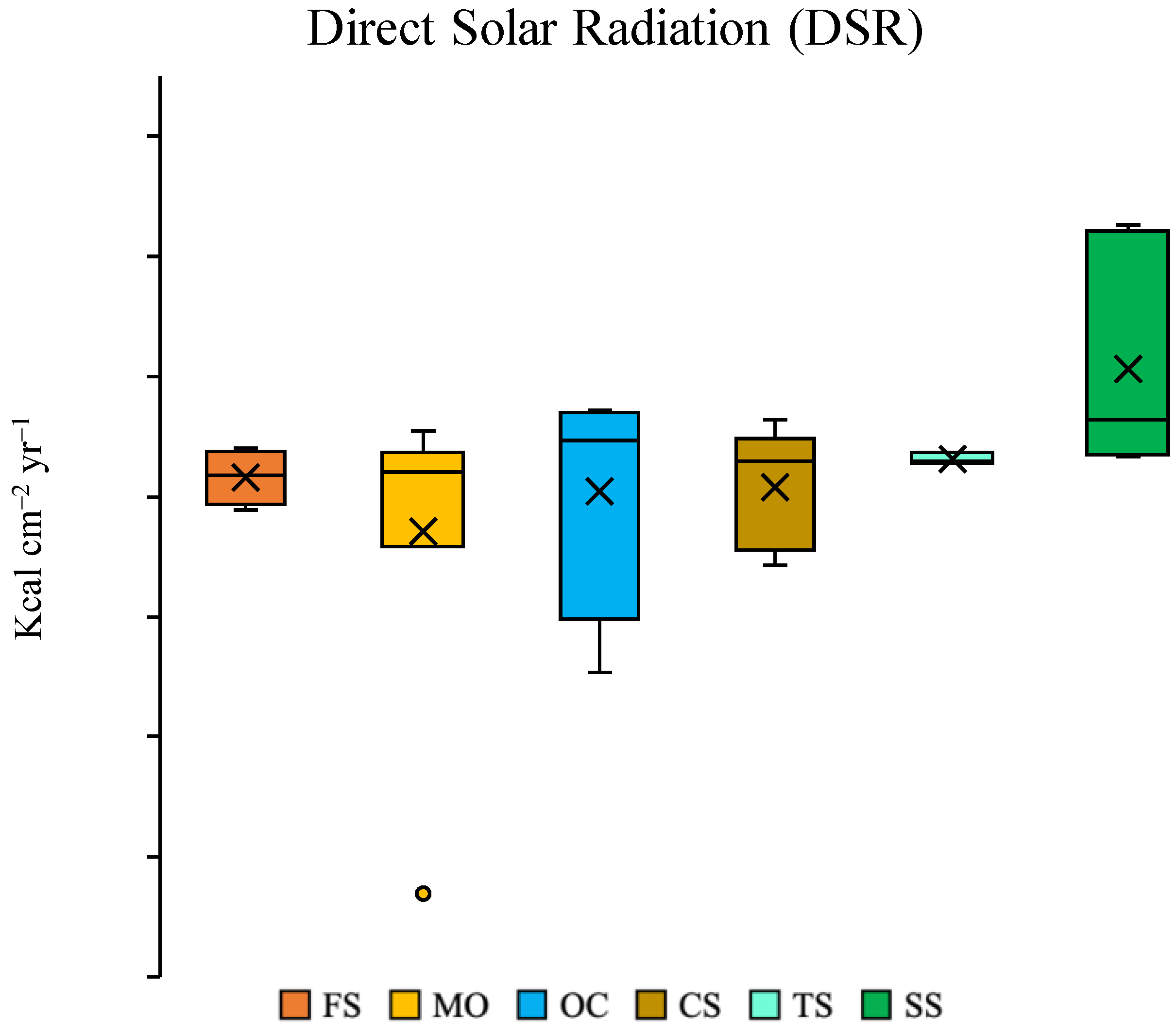
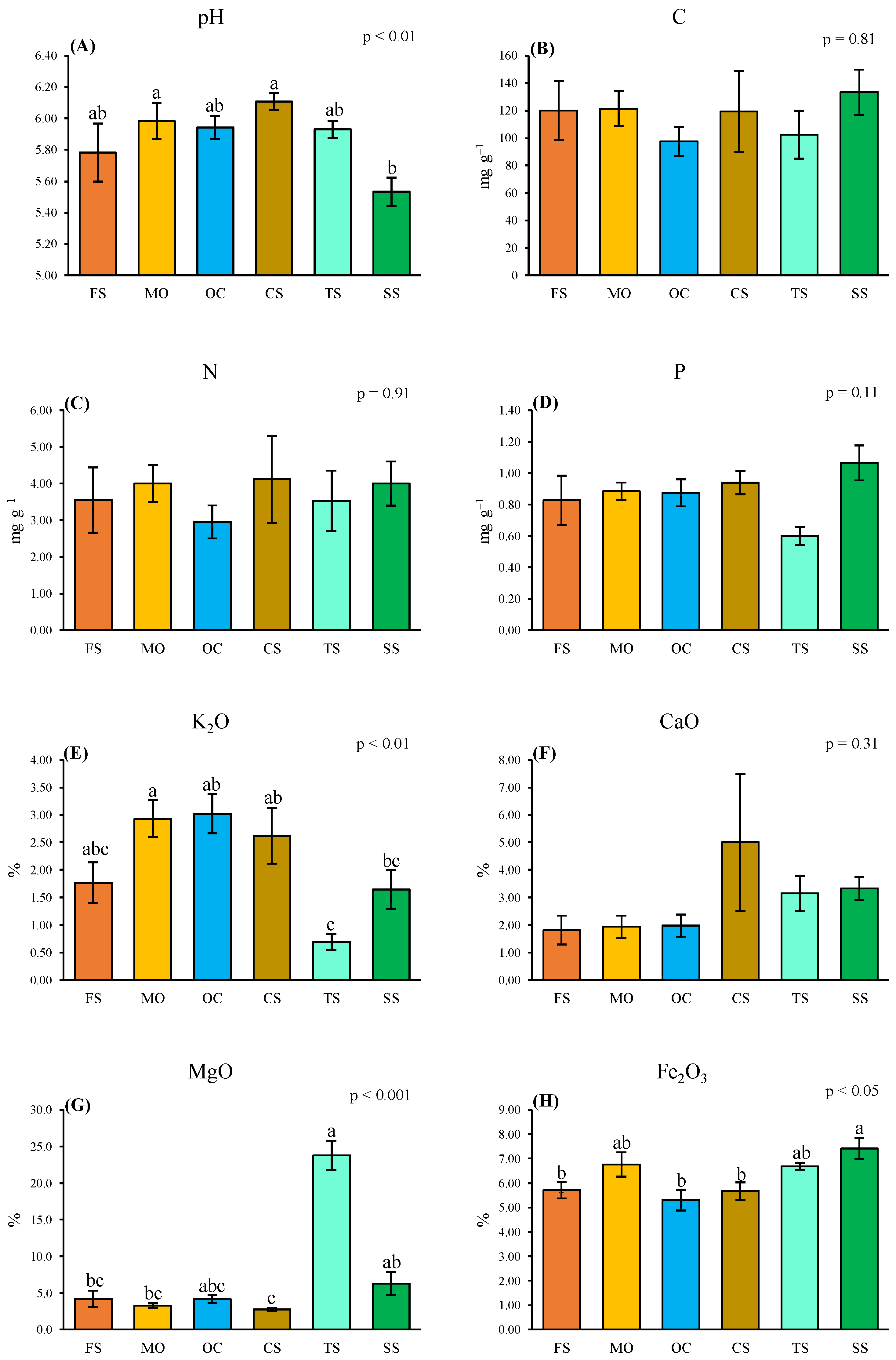
2.3. Direct Solar Radiation (DSR) and Soil Chemistry

Although there were no overall differences among lithological types in terms of DSR (F5,24 = 1.69; p = 0.17), the mean DSR was significantly different (F1,12 = 4.94; p < 0.05) between the highest value in SS and the lowest value in MO (Figure 2). The soil VWC also differed significantly (F1,12 = 18.74; p < 0.001) between these two lithological types with a higher value in MO (11.3 ± 1.3%) than in SS (5.1 ± 0.5%).
The soil pH differed among the lithological groups, with the SS soils being significantly more acidic than the CS and MO soils (Figure 3A). The K concentration was highest in MO, OC, and Cs; intermediate in FS and SS; and lowest in TS (Figure 3E). The Mg concentration was distinctly higher in TS (Figure 3G) and the Fe concentration was slightly higher in SS than in the other lithological groups (Figure 3H). The concentrations of C, N, P, and Ca were more or less the same in all lithological groups (Figure 3B–D,F).

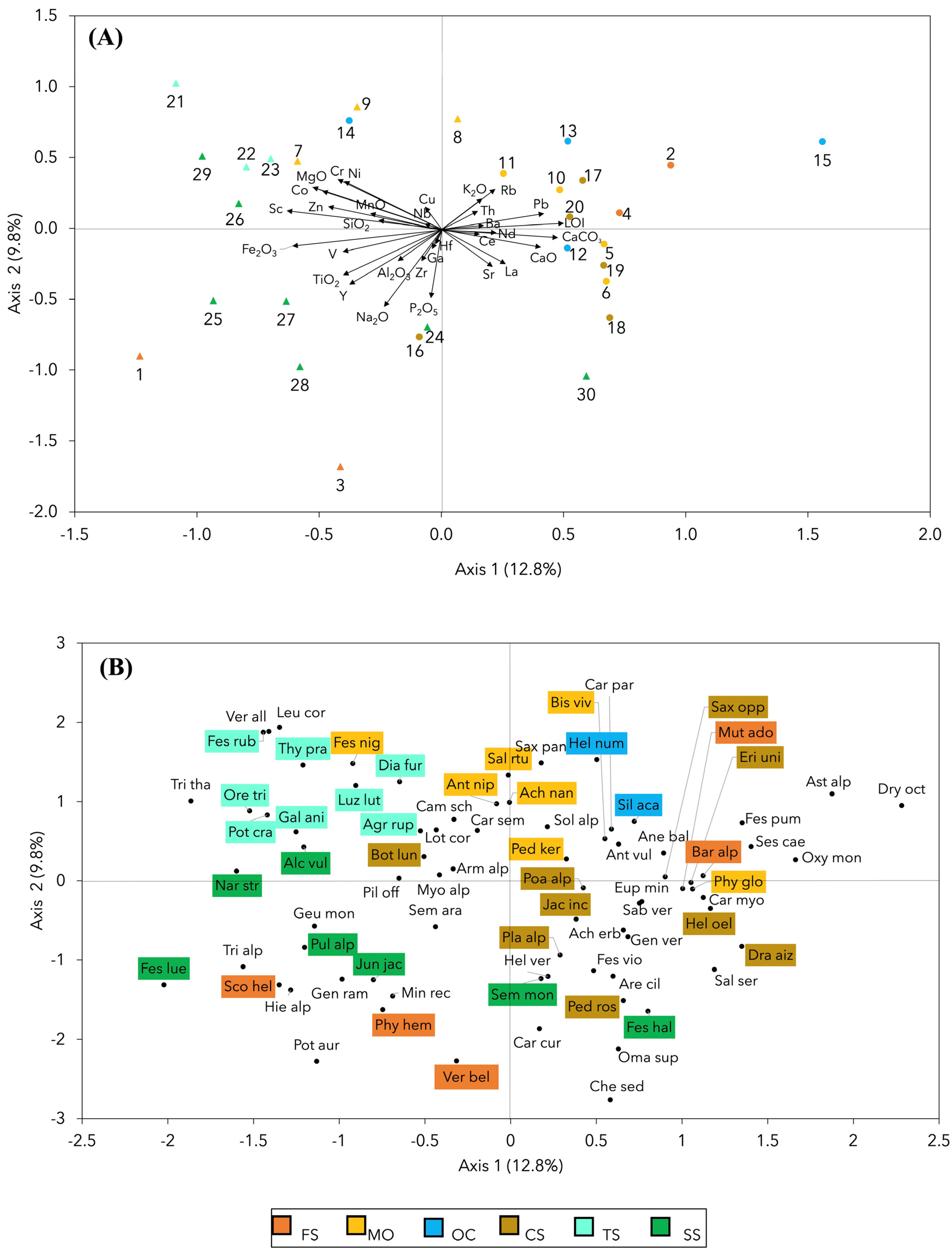
2.4. Vegetation and Its Relationships with the Lithological Groups and Bedrock Chemistry

In total, 137 species were recorded, of which 76 were present in 3 or more plots (Table 2). The other 61 species were considered ‘occasional species’ and are listed in Supplementary Table S3. On the basis of the IndVal index, 38 species were identified, among which 9 were highly indicative (p < 0.01; Table 2). The indicator species are listed below.
-
FS indicator species: Bartsia alpina, Mutellina adonidifolia, Phyteuma hemisphaericum, Scorzoneroides helvetica, and Veronica bellidioides.
-
MO indicator species: Achillea nana, Pedicularis kerneri, Salix retusa, Anthoxanthum nipponicum, Festuca nigricans, and Bistorta vivipara.
-
OC indicator species: Helianthemum nummularium subsp. grandiflorum, and Silene acaulis.
-
CS indicator species: Helianthemum oelandicum subsp. alpestre, Botrychium lunaria, Draba aizoides subsp. aizoides, Erigeron uniflorus, Pedicularis rosea subsp. allionii, Phyteuma globulariifolium subsp. pedemontanum, Plantago alpina, Poa alpina, Saxifraga oppositifolia subsp. oppositifolia, and Jacobaea incana.
-
TS indicator species: Luzula lutea subsp. lutea, Potentilla crantzii subsp. crantzii, Thymus praecox subsp. polytrichus, Agrostis rupestris subsp. rupestris, Dianthus furcatus, Festuca rubra, Galium anisophyllon, and Oreojuncus trifidus.
-
SS indicator species: Juncus jacquinii, Alchemilla vulgaris, Festuca halleri, Festuca scabriculmis subsp. luedii, Nardus stricta, Pulsatilla alpina subsp. apiifolia, and Sempervivum montanum.
The first two CCA axes (Figure 4A,B) collectively accounted for 22.6% of the total variance. The ordination of the plots along the first CCA axis was mainly associated with increasing concentrations of CaO, CaCO3, L.O.I. and Pb towards the right end of the biplot. In contrast, the Fe2O3 vector had an opposite orientation, directed towards the left end of the biplot (Figure 4A). The ordination of species (Figure 4B) along the first CCA axis generally reflected a soil pH gradient, with calcifuge species having negative scores and calcicole species positive scores on the first CCA axis. However, species ordination along the first CCA axis only partly reflected associations between species and lithological groups. Notably, all calcicole species at the right end of the gradient (Dryas octopetala subsp. octopetala, Aster alpinus subsp. alpinus, Festuca pumila, Oxytropis montana, and Sesleria caerulea) did not represent indicator species for any lithological group. However, most CS indicator species represented moderately calcicole species with positive scores on the first CCA axis. This was especially the case for Draba aizoides subsp. aizoides, Helianthemum oelandicum subsp. alpestre, Erigeron uniflorus, and Saxifraga oppositifolia subsp. oppositifolia. Other CS indicator species presented only weakly calcicole characteristics (Pedicularis rosea subsp. allionii, Phyteuma globulariifolium subsp. pedemontanum, and Poa alpina) or even more or less strongly calcifuge characteristics (Plantago alpina, Jacobaea incana, and Botrychium lunaria). Consistently, these species had less positive or even slightly negative scores on the first CCA axis (Figure 4B). Further mutual relationships of plant species and plots in relation to bedrock chemistry were revealed by the combined scores on the two CCA axes. The TS indicator species (Agrostis rupestris subsp. rupestris, Dianthus furcatus, Festuca rubra, Galium anisophyllon, Oreojuncus trifidus, Luzula lutea subsp. lutea, Potentilla crantzii subsp. crantzii, and Thymus praecox subsp. polytrichus) and all TS plots were located in the upper left sector of the diagram, i.e., the side towards which the vectors of Ni, Cr, Co, Zn, Sc, and MgO were oriented (Figure 4A,B). The MO plots were distributed in a wide range of scores on the first CCA axis with an overall poor association with the vectors of the bedrock chemistry variables, except Rb and to a lesser extent K2O (Figure 4A). The MO indicator species (Achillea nana, Anthoxanthum nipponicum, Festuca nigricans, Pedicularis kerneri, Bistorta vivipara, and Salix retusa) were also distributed in a wide range in the upper sector of the diagram (Figure 4B). The SS plots were located in the lower left sector of the diagram in close association with the Fe2O3, V, TiO2 and Y vectors, as well as with most SS indicator species (Alchemilla vulgaris, Festuca scabriculmis subsp. luedii, Juncus jacquinii, Nardus stricta, Pulsatilla alpina subsp. apiifolia, and Sempervivum montanum) with the exception of Festuca halleri which was located in the lower right sector of the diagram (Figure 4A,B). The OC plots were mostly located in the upper right sector of the diagram which reflected their quite high CaO and CaCO3 contents and also the high L.O.I., although all were slightly lower than those of the CS (Table 1). The two OC indicator species (Helianthemum nummularium subsp. grandiflorum, and Silene acaulis) were also located in the upper right sector of the diagram (Figure 4A,B). The reciprocal ordination of the FS plots and their indicator species reflected the heterogeneity of this lithological group in terms of bedrock chemistry, soil pH, and species composition. In fact, plots 1 and 3 were located in the lower left sector of the diagram, i.e., the side towards which the vectors of SiO2, Al2O3, TiO2, Na2O, and P2O5 were oriented (Figure 4A). These two FS plots were characterized by acidic pH and, consistently, by the presence of three calcifuge indicator species (Phyteuma hemisphaericum, Scorzoneroides helvetica, and Veronica bellidioides), also located in the lower left sector of the diagram (Table 2 and Figure 4B). On the contrary, plots 2 and 4 were located in the upper right sector of the diagram in association with the Ce and La vectors. These two plots had higher pH and were characterized by the indicator species Bartsia alpina and Mutellina adonidifolia, which are slightly calcicole or indifferent (Table 2 and Figure 4B).

3. Discussion

The vegetation of the grasslands analyzed in our study was not distinctive of calc-schists s.l. or serpentines s.l. Indeed, most of the species recorded in our plots are considered characteristic of alpine grasslands which comprise a range of plant communities across mountain ranges and arctic regions in Europe. The majority of these species characterize the alpine and subalpine silicicolous or calcicolous communities of the mountain ranges in the nemoral zone of Europe (Caricetalia curvulae and Seslerietalia caeruleae, respectively [26]). A minority of the remaining species characterize alpine habitats other than true grasslands [26]: relict summit graminoid tundra in the alpine and subnival belts (Oxytropido-Elynetalia); subnival and alpine lime-rich shale screes and frozen slopes of the Alps and the Pyrenees of the nemoral mountain ranges (Drabetalia hoppeanae); snow-beds on stabilized calcareous screes of the arctic zone and the alpine and subnival belts of European mountains (Arabidetalia caeruleae); arctic and alpine subnival snow-beds at high altitudes of the mountain ranges of Eurasia and the Arctic Ocean islands (Salicetalia herbaceae). About one-fifth of the species are characteristic of other syntaxa, not specifically related to alpine habitats (Table 2). This confirms the results of previous studies reporting the lack of distinctive vegetation types in alpine grasslands on calc-schist s.l. or serpentine s.l. bedrocks in the Western Alps [27,28]. The only distinctive plant community in the serpentine alpine habitats of the Western Alps is the Caricetum fimbriatae. However, this community is generally located in the upper parts of stabilized screes and especially in rock crevices where the character species Carex fimbriata is often associated with the chasmophyte Cardamine plumieri [29]. These habitats were outside the alpine grasslands sampled in our study. Consistently, Carex fimbriata was never recorded in our plots. There was no clear separation between calcifuge and calcicole species on calc-schist s.l. and serpentine s.l. bedrocks. Calcifuge species, characteristic of Caricetalia curvulae, were overall more frequent in the more acidic serpentine plots. However, among the frequent species (i.e., occurring in at least 30% of the plots) of Caricetalia curvulae, only Oreojuncus trifidus and Trifolium alpinum were present exclusively, or almost exclusively, in the serpentine s.l. plots. The typical species of Caricetalia curvulae, such as Carex curvula subsp. curvula and Helictotrichon versicolor subsp. versicolor, were even recorded with equal frequency in the two main bedrock types. A slightly higher number of calcicole species characteristic of Seslerietalia caeruleae (Helianthemum oelandicum subsp. alpestre, Sesleria caerulea, Anthyllis vulneraria subsp. alpicola, and Oxytropis montana) or Oxytropido-Elynetalia (Dryas octopetala subsp. octopetala and Carex myosuroides) were much more frequent in, or entirely excusive of, the calc-schist s.l. plots. Also in this case, none of these species characterize the vegetation of calc-schists s.l. or serpentines s.l. since they are widespread in alpine plant communities on siliceous bedrocks such as granite and gneiss, especially Caricetum curvulae, or carbonate rocks, especially Seslerio-Caricetum sempervirentis, Caricetum firmae, and Elynetum myosuroidis, respectively [30].
The aim of our study was precisely to investigate whether and to what extent a detailed geochemical and petrographic analysis, beyond the dichotomous distinction between calc-schists s.l. and serpentines s.l., could be effective for a fine characterization of alpine grasslands based on species composition. The overall geological complexity of the Western Alps was partially reflected in our lithological samples, which presented considerable geochemical heterogeneity including both continental and ophiolitic nappes, known as the Penninic domain [31]. The so-called ophiolitic basement nappes exhibit a high-grade metamorphism and are overlain by a relatively wide array of metasediments ranging from calc-schists to marbles, quartzites, black schists, shales, metabasites, metaophicalcites, and radiolarian cherts [32,33]. In the geographic context of the Penninic domain of the Western Alps, three macro-categories of ophiolites were identified [34]: (1) ultramafic peridotitic rocks from the asthenosphere, mostly serpentinized by hydrothermal metamorphism into serpentinites; (2) mafic rocks such as metagabbros and metabasalts, both originating from the ocean crust and presenting inclusions of micas and feldspar; (3) pelagic metasediments, both siliceous and calcareous (e.g., calc-schists, ophicalcites and serpentine breccias with calcareous cement). Therefore, the definition of ophiolites lacks geochemical homogeneity due to the substantial differences between crustal and mantle rocks, which impose different constraints on the vegetation [35]. The two lithological groups entirely made up of plots assigned to serpentines s.l., viz. TS and SS, were both quite well characterized in terms of species composition. In particular, TS was characterized by Galium anisophyllon, a species of metallicolous vegetation (Galio anisophylli-Minuartion vernae) from central Europe [36]. Sabulina verna (=Minuartia verna). Another character species of Galio anisophylli-Minuartion vernae, was also present in one of the TS plots but it was absolutely not an indicator species of TS because it was also recorded with equal frequency in OC and CS. Furthermore, TS was also characterized by Luzula lutea subsp. lutea, considered as a serpentine indicator in the Western Alps [37]. These vegetation characteristics are consistent with the bedrock geochemistry in TS, which had high concentrations of MgO and heavy metals, especially Co, Cr, and Ni. The latter reflect the high heavy metal contents detected in serpentine soils of different regions across the world [38,39,40,41,42]. Although none of these three species are limited to serpentine grasslands, all can behave as heavy metal accumulators [43,44] which have evolved physiological mechanisms to tolerate heavy metal toxicity [45,46,47]. The soil chemistry reflected the geochemical characteristics of the TS bedrock. Although our study did not aim to assess the availability of individual elements to plants, which would require analysis of extractable elements [38], the total concentrations of major nutrients in the TS soils provided evidence of P and especially K limitation as often observed in serpentine soils [48]. Some of the TS indicator species were also present in SS, although with lower frequencies, in agreement with the lower contents of MgO and heavy metal in the SS bedrock compared to that of TS. On the other hand, the SS indicator species, especially Festuca scabriculmis subsp. luedii, are typical of alpine grasslands developed on steep slopes with stony and dry soils, as evidenced by the high DSR and low soil VWC in the SS plots. This vegetation resembled that of alpine grasslands on steep arid south-facing slopes developed on different types of siliceous bedrocks, such as granite, gneiss, porphyry, and others, in several sectors of the Alps. The vegetation of these grasslands is characterized by taxonomically closely related calcifuge taxa of the Festuca varia group [49,50]. This suggests that other factors in addition to bedrock chemistry, i.e., solar radiation input and soil water content, could explain some degree of variation in the species composition of the alpine grasslands considered in our study.
The two lithological groups entirely composed of plots assigned to calc-schists s.l., viz. OC and CS, were quite well characterized in terms of species composition: Carex myosuroides, Carex curvula subsp. curvula, and Helianthemum oelandicum subsp. alpestre (the latter especially in CS) were among the most frequent species in the vegetation of these two lithological groups. All of them are dominant in alpine grasslands on calc-schists in the Vanoise Massif of the French Alps, near the Italian border [51]. In the calc-schist grasslands of the Vanoise, Carex curvula subsp. rosae has generally been recorded, while in our plots only Carex curvula subsp. curvula was present. Among the CS indicator species, Saxifraga oppositifolia subsp. oppositifolia and Poa alpina were of great importance because they characterize the vegetation of cryoturbated alpine habitats on calc-schist bedrock in the Western Pennine Alps in Switzerland [52]. Furthermore, the set of the CS indicators included three calcicole species which represent diagnostic species of stabilized alpine debris on calc-schist bedrock (order Drabetalia hoppeanae): Phyteuma globulariifolium subsp. pedemontanum, Erigeron uniflorus, and Draba aizoides subsp. aizoides [53]. Some of the CS indicator species were also occasionally found in OC, but the most distinctive indicator species for OC was Silene acaulis, a cushion species widespread throughout the Northern Hemisphere on different types of bedrocks [54,55]. The vegetation characteristics described above were consistent with the distinctive geochemical signature of the OC and CS bedrock, characterized by high CaO and CaCO3 contents with peak values in CS. This supports the results of other studies that have focused on carbonate content as the main driver of variation in alpine vegetation [56,57]. FS and MO had the common characteristic of sialic rocks, consisting of high contents of SiO2, Al2O3, and K2O. Apart from this, both lithological groups were petrologically heterogeneous to the point of including plots classified both as serpentines s.l. and calc-schists s.l. This heterogeneity was reflected by the vegetation characteristics of FS and MO. The FS indicators consisted mainly of calcifuge species characteristic of Caricetalia curvulae: Phyteuma hemisphaericum, Scorzoneroides helvetica, and Veronica bellidioides. The MO indicators were ecologically more heterogeneous, with calcifuge species typical of Caricetalia curvulae (Pedicularis kerneri) associated with calcicole species typical of Seslerietalia caeruleae (Festuca nigricans) and moderately calcicole species typical of stabilized calc-schist screes of Drabetalia hoppeanae (Achillea nana). This is consistent with the bedrock chemistry in MO, presenting higher CaO and CaCO3 contents compared to FS. This, once again, underlines the important role that carbonate content plays in structuring alpine vegetation, not necessarily correlated with soil pH [56]. Interestingly, the set of MO indicators also included Salix retusa, a dwarf-willow characterizing snow-bed vegetation on carbonate soils (Arabidetalia caeruleae; [58]). An additional MO indicator, which was present in all MO plots, was Bistorta vivipara. Bistorta vivipara is a widespread species found in several alpine plant communities but is particularly frequent in snow-beds where it is enhanced by meltwater that saturates the soil at the beginning of the growing season [59]. Similar to what was observed for SS, this suggests that environmental factors unrelated to bedrock chemistry, in this case snow cover duration, which is in turn related to lower solar radiation input and higher soil VWC, were responsible for a degree of variation in the investigated alpine grasslands.

4. Materials and Methods

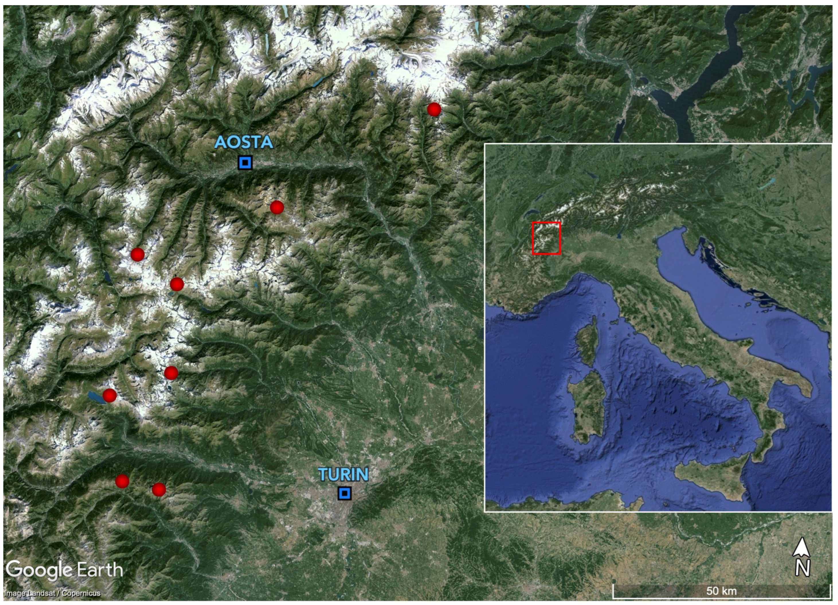
4.1. Study Area, Sampling Design, and Data Collection

Our goal was to sample a region large enough to cover the widest possible range of geographic variation in the petrographic composition of the two bedrock types examined. With this objective in mind, we selected eight sites in alpine grasslands in a region ranging between the northern Cottian Alps, the whole Graian Alps, and the middle Pennine Alps (Figure 5). These sites were chosen after a careful inspection of geological maps [24] which allowed us to select a series of sites where rather vast outcrops of serpentines, calc-schists, or both bedrock types were present. At each of the 8 sites we selected 3 to 6 1 × 1 m square plots, for a total of 30 plots. The small size of the sampling plots was justified by the need to sample petrographically homogeneous plots because it is known that rock and soil chemistry can present small-scale variation in relation to microtopography [60]. The choice of the sampling plots was based on a careful visual inspection of the sites. All plots were located at 2500 ± 100 m above sea level, on flat or moderately inclined terrain (maximum slope inclination of 35°), thus limiting the sampling area to the mid-alpine vegetation belt, i.e., where the alpine grasslands thrive and reach their late successional stages. At each site, the location of the plots covered the whole range of aspects where appropriate areas were found, in most cases all four cardinal points. Regarding vegetation structure, all plots were located in areas where vegetation covered at least 50% of the ground but vegetation cover generally was >60%. Only areas covered by low stature vegetation were considered, i.e., with a maximum total shrub cover < 10%, except for dwarf willows (Salix herbacea, S. reticulata, S. retusa, S. serpillifolia) and alpine azalea (Kalmia procumbens). The nomenclature of the species follows the Portal to the Flora of Italy [61].
The field sampling was carried out during the period 12–27 July 2022. The cover of all vascular species was estimated visually at each plot using the following categorical scale: 1, cover 1–10%; 2, cover 11–20%; 3, cover 21–30%; 4, cover 31–40%; 5, cover 41–50%; 6, cover 51–60%; 7, cover 61–70%; 8, cover 71–80%; 9, cover: 81–90%; 10, cover: 91–100%. Geographic coordinates, elevation, aspect, and slope angle were determined at each plot by a GPS and a compass. At some plots we also determined soil volumetric water content (VWC) using a FieldScout time domain reflectometer TDR 100 Soil Moisture Meter (Spectrum Technologies Inc., Aurora, IL, USA). At each plot, a rock sample was collected from natural outcrops and about 100 g of the top soil was collected as well. All plots had very shallow soils. Thus, soil sampling was carried out by removing the top 1 cm layer and then collecting the soil to a maximum depth of 5 cm, which is the depth to which almost all plants root. The soil sample for a given plot consisted of composite material collected from at least five points spread over the 1 × 1 m2.

4.2. Bedrock and Soil Analyses

The bedrock analyses were carried out at the Department of Physics and Earth Sciences of Ferrara University. The rock samples were examined under a stereomicroscope to obtain a detailed description of the mineral structure. A rock subsample was pulverized with an agate pestle and three aliquots were assigned to different analyses: the first aliquot was used for calcimetric analyses that evaluated the CaCO3 content by the gas volumetric method; the second aliquot was used to calculate L.O.I (loss on ignition); the third aliquot was incorporated into a tablet prepared with a boric acid support in order to determine concentrations of major and trace elements by X-ray fluorescence (X.R.F.) analysis using a wavelength-dispersive ARL Advant’XP X-ray fluorescence spectrometer (Thermo Fisher Scientific, Waltham, MA, USA). The main elements were expressed as percentage of oxide weight (SiO2, TiO2, Al2O3, Fe2O3, MnO, MgO, CaO, Na2O, K2O, P2O5). Concentrations of trace elements (Ba, Ce, Co, Cr, Cu, Ga, Hf, La, Nb, Nd, Ni, Pb, Rb, Sc, Sr, Th, V, Y, Zn and Zr) were expressed as mg kg−1. The entire matrix correction procedure and the intensities were elaborated according to Lachance and Traill [62]. The accuracy of the instrumentation was estimated on the basis of the results obtained from international standards of geological samples, and the precision was expressed as standard deviation of replicated analyses. Accuracy and precision were >2–5% for major elements and 5–10% for trace elements. The detection limit was 0.01% for the main oxides and 1–3 mg kg−1 for trace element concentrations, respectively.
The soil analyses were carried out at both the Laboratory of Plant Ecology (Department of Environmental and Prevention Sciences) and the Department of Physics and Earth Sciences of Ferrara University of Ferrara University. A 10 g subsample of dry soil was extracted in a 1:2.5 (vol/vol) aqueous solution and used to determine soil pH with a pH meter [Hanna Edge, Villafranca Padovana (PD), Italy]. A 500 mg subsample of dry soil, sieved with a 0.125 mm mesh, was used for analyzing total carbon (C) by a Shimadzu TOC-VCSH (Shimadzu Corporation; Kyoto, Japan), connected with a solid sample module (Shimadzu SSM-5000A). A 200 mg subsample of dry soil, sieved with a 0.125 mm mesh, was extracted in 3 mL of selenous H2SO4 at 420 °C and analyzed for total nitrogen (N) concentration using the salicylate method, and for total phosphorus (P) concentration by the molybdenum blue method using a continuous flow autoanalyzer (FlowSys; Systea, Anagni, Italy). To determine total soil concentrations of K (as K2O), Ca (as CaO), Mg (as MgO), and Fe (as Fe2O3), a subsample of soil was sieved and subsequently pulverized using an agate mortar and subsequently embedded in a tablet for the X.R.F. analysis, as for the bedrock analyses.

4.3. Data Compilation and Statistical Analyses

The cumulative direct solar radiation (DSR) input at each plot was calculated by combining field-measured slope angle and aspect data according to Buffo et al. [63]. In the calculations, we assumed a linear trend of DSR values between slope increments. Then, we algebraically interpolated DSR values for intermediate slope angles at latitudes of 40° and 50° N. Further assuming a linear trend of latitudinal DSR values, we estimated DSR at latitude of 45° N by averaging the corresponding DSR values at latitudes of 40° and 50° N, respectively. Elevation was not included in the calculations due to the narrow elevation range of our plots.
A geochemical bedrock classification was obtained through cluster analysis of 32 geochemical variables using the Ward’s method based on the Euclidean distance. In order to avoid biases associated with the wide range of concentrations among the variables considered, the raw values were normalized to the maximum value using Formula (1):
Xnormalized = Xi/Xmax
where Xi is the rough value of a given variable for a plot site and Xmax is the maximum rough value of a given variable across the whole set of plots.
The significance of differences among lithological clusters in terms of bedrock chemistry and soil chemistry was assessed by one-way ANOVAs and Dunn’s post hoc tests. The relationships between vegetation and bedrock chemistry were analyzed by Canonical Correspondence Analysis (CCA). To measure the association between species composition and lithological clusters, we used the Indicator Value (IndVal) index [64]. The IndVal index combines the average relative abundance and frequency of species occurrence in the lithological groups. We considered two classes of significance for the indicator species based on the p values associated to the IndVal: p < 0.05 and p < 0.01. The statistical analyses were performed using the software Past 4.13 [65].

5. Conclusions

We conclude that the vegetation investigated in our study was mostly made up of a set of species found more or less frequently found in silicicolous or calcicolous alpine plant communities in the Alps and other European mountains. Overall, there were no distinctive species uniquely characterizing grassland vegetation on serpentines s.l. or calc-schists s.l. Bedrock carbonate content was a major driver of variation in grassland vegetation, not necessarily related to soil pH. Detailed petrological analyses of bedrock revealed subtle differences in species composition associated with a complex interplay between protolith geochemistry, lithological genesis, and degree of metamorphism. Other factors additional to bedrock chemistry, in particular solar radiation and soil moisture content, also played a role in structuring the vegetation of alpine grasslands.

Supplementary Materials

The following supporting information can be downloaded at: https://www.mdpi.com/article/10.3390/plants13162280/s1, Table S1: Location of the plots with description of the lithotypes as listed in the Geological maps, Table S2: Synthetic petrological overview of the six lithological groups, Table S3: List of the rare species.

Author Contributions

Conceptualization, A.C., R.G. and L.B.; field investigation, R.G. and L.B.; geochemical and petrological analyses, E.M. and C.V.; writing—original draft, A.C. and R.G.; writing—review and editing, A.C. and R.G. All authors have read and agreed to the published version of the manuscript.

Funding

This publication was funded by the University of Ferrara (grant FIRD 2022, resp. LB).

Data Availability Statement

The data presented in this study are available upon request from the corresponding author. The data are not publicly available due to privacy.

Conflicts of Interest

The authors declare no conflicts of interest.

References

  1. Poulenard, J.; Podwojewski, P. Alpine soils. In Encyclopedia of Soil Science; Chesworth, W., Ed.; Marcel Dekker: New York, NY, USA, 2003; pp. 1–4. [Google Scholar]
  2. Väre, H.; Lampinen, R.; Humphries, C.; Williams, P. Taxonomic diversity of vascular plants in the European alpine areas. In Alpine Biodiversity in Europe; Körner, C., Grabherr, G., Nagy, L., Thompson, D.B.A., Eds.; Springer: Berlin/Heidelberg, Germany, 2003; pp. 133–148. [Google Scholar]
  3. Ellenberg, H. The vegetation above the alpine tree line. In Vegetation Ecology of Central Europe, 4th ed.; Cambridge University Press: Melbourne, Australia, 1988; pp. 388–455. [Google Scholar]
  4. Leuschner, C.; Ellenberg, H. Vegetation of the alpine and nival belts. In Ecology of Central European Nonforest Vegetation: Coastal to Alpine, Natural to Man-made Habitats: Vegetation Ecology of Central Europe; Springer Nature: Cham, Switzerland, 2017; Volume 2, pp. 271–431. [Google Scholar]
  5. Körner, C. Concepts in alpine plant ecology. Plants 2023, 12, 2666. [Google Scholar] [CrossRef]
  6. Braun-Blanquet, J.; Jenny, H. Vegetationsentwicklung und Bodenbildung in der alpinen Stufe der Zentralalpen (Klimaxgebiet des Caricion curvulae). Mèmoires Société Helvétique Sci. Nat. 1926, 63, 183–349. [Google Scholar]
  7. Gigon, A. Vergleich alpiner Rasen auf Silikat- und auf Karbonatboden: Konkurrenz- und Stickstofformen Versuche sowie standörtliche Untersuchungen im Nardetum und im Seslerietum bei Davos. Veröffentlichungen Geobot. Inst. Eidg. Techn. Hochsch. Stift. Rübel 1971, 48, 1–159. [Google Scholar]
  8. Reisigl, H.; Keller, R. Alpenpflanzen im Lebensraum (Alpine Rasen, Schuttund Felsvegetation); Gustav Fischer Verlag: Stuttgart, Germany, 1987; 149p. [Google Scholar]
  9. Tyler, G. Some ecophysiological and historical approaches to species richness and calcicole/calcifuge behaviour—Contribution to a debate. Folia Geobot. 2003, 38, 419–428. [Google Scholar] [CrossRef]
  10. Lee, J.A. The calcicole-calcifuge problem revisited. Adv. Bot. Res. 1999, 29, 2–30. [Google Scholar]
  11. Zohlen, A.; Tyler, G. Immobilization of tissue iron on calcareous soil: Differences between calcicole and calcifuge plants. Oikos 2000, 89, 95–106. [Google Scholar] [CrossRef]
  12. Zohlen, A.; Tyler, G. Soluble inorganic tissue phosphorus and calcicole–calcifuge behaviour of plants. Ann. Bot.-London 2004, 94, 427–432. [Google Scholar] [CrossRef]
  13. Lambers, H.; Hayes, P.E.; Laliberté, E.; Oliveira, R.S.; Turner, B.L. Leaf manganese accumulation and phosphorus-acquisition efficiency. Trends Plant Sci. 2015, 20, 83–90. [Google Scholar] [CrossRef] [PubMed]
  14. de Souza, M.C.; Habermann, G.; do Amaral, C.L.; Rosa, A.L.; Ongaro Pinheiro, M.H.; Da Costa, F.B. Vochysia tucanorum Mart.: An aluminum-accumulating species evidencing calcifuge behavior. Plant Soil 2017, 419, 377–389. [Google Scholar] [CrossRef]
  15. Hayes, P.E.; Guilherme Pereira, C.; Clode, P.L.; Lambers, H. Calcium-enhanced phosphorus toxicity in calcifuge and soil-indifferent Proteaceae along the Jurien Bay chronosequence. New Phytol. 2019, 221, 764–777. [Google Scholar] [CrossRef]
  16. Wala, M.; Kolodziejek, J.; Mazur, J. The diversity of iron acquisition strategies of calcifuge plant species from dry acidic grasslands. J. Plant Physiol. 2023, 280, 153898. [Google Scholar] [CrossRef] [PubMed]
  17. Kovács, G.; Radovics, B.G.; Tóth, T.M. Petrologic comparison of the Gyód and Helesfa serpentinite bodies (Tisia Mega Unit, SW Hungary). J. Geosci.-Czech 2016, 61, 255–279. [Google Scholar] [CrossRef]
  18. Wakabayashi, J. Serpentinites and serpentinites: Variety of origins and emplacement mechanisms of serpentinite bodies in the California Cordillera. Island Arc. 2017, 26, e12205. [Google Scholar] [CrossRef]
  19. Burianek, D.; Pertoldova, J. Garnet-forming reactions in calc-silicate rocks from the Policka Unit, Svratka Unit and SE part of the Moldanubian Zone. J. Geosci.-Czech 2009, 54, 245–268. [Google Scholar] [CrossRef]
  20. Nabelek, P.I.; Morgan, S.S. Metamorphism and fluid flow in the contact aureole of the Eureka Valley–Joshua Flat–Beer Creek pluton, California. Geol. Soc. Am. Bull. 2012, 124, 228–239. [Google Scholar] [CrossRef]
  21. Pfiffner, A. Geology of the Alps; Wiley-Blackwell: Hoboken, NJ, USA, 2014; 376p. [Google Scholar]
  22. Lagabrielle, Y.; Cannat, M. Alpine Jurassic ophiolites resemble the modern central Atlantic basement. Geology 1990, 18, 319–322. [Google Scholar] [CrossRef]
  23. Fioraso, G.; Balestro, G.; Festa, A.; Lanteri, L. Role of structural inheritance in the gravitational deformation of the Monviso meta-ophiolite complex: The Pui-Orgiera serpentinite landslide (Varaita Valley, Western Alps). J. Maps 2019, 15, 372–381. [Google Scholar] [CrossRef]
  24. Geological Map of Italy, Scale 1:100,000, Sheets n. 28, 29, 41, 55; Geological Survey of Italy. Available online: https://sgi.isprambiente.it/geologia100k/nord.aspx (accessed on 30 April 2024).
  25. Ague, J.J. Element mobility during regional metamorphism in crustal and subduction zone environments with a focus on the rare earth elements (REE). Am. Mineral. 2017, 102, 1796–1821. [Google Scholar] [CrossRef]
  26. Mucina, L.; Bültmann, H.; Dierßen, K.; Theurillat, J.P.; Raus, T.; Čarni, A.; Šumberová, K.; Willner, W.; Dengler, J.; Gavilán García, R.; et al. Vegetation of Europe: Hierarchical floristic classification systemof vascular plant, bryophyte, lichen, and algal communities. Appl. Veg. Sci. 2016, 19, 3–264. [Google Scholar] [CrossRef]
  27. Vercesi, G.V. Valutazioni ecologiche sulla flora e sulla vegetazione delle ofioliti della Valmalenco (SO). Rev. Valdôtaine Hist. Nat. 2004, 58, 121–128. [Google Scholar]
  28. Mainetti, A.; Ravetto Enri, S.; Lonati, M. Vegetation trajectories in proglacial primary successions within Gran Paradiso National Park: A comparison between siliceous and basic substrates. Ibex-J. Mt. Ecol. 2022, 14, 1–18. [Google Scholar]
  29. Verger, J.P. Premières considerations sur la végétation alpine et les sols developpés sur serpentinites, prasinites et gabbros dans les Alpes Graies (Italie). Webbia 1993, 47, 313–328. [Google Scholar] [CrossRef]
  30. Pignatti, E.; Pignatti, S. Plant Life of the Dolomites. Vegetation Structure and Ecology; Springer: Berlin/Heidelberg, Germany, 2014; p. 769. [Google Scholar]
  31. Dal Piaz, G.V.; Bistacchi, A.; Massironi, M. Geological outline of the Alps. Episodes J. Int. Geosci. 2003, 26, 175–180. [Google Scholar] [CrossRef] [PubMed]
  32. Principi, G.; Bortolotti, V.; Chiari, M.; Cortesogno, L.; Gaggero, L.; Marcucci, M.; Saccani, E.; Treves, B. The pre-orogenic volcano-sedimentary covers of the western Tethys oceanic basin: A revue. Ofioliti 2004, 29, 177–211. [Google Scholar]
  33. Tartarotti, P.; Martin, S.; Festa, A.; Balestro, G. Metasediments covering ophiolites in the HP internal belt of the Western Alps: Review of tectono-stratigraphic successions and constraints for the Alpine evolution. Minerals 2021, 11, 411. [Google Scholar] [CrossRef]
  34. Prinetti, F. Brevi note per i botanici sulle rocce ofiolitiche. Rev. Valdôtaine Hist. Nat. 2004, 58, 5–6. [Google Scholar]
  35. Proctor, J.; Woodell, S.R. The plant ecology of serpentine: I. Serpentine vegetation of England and Scotland. J. Ecol. 1971, 59, 375–395. [Google Scholar] [CrossRef]
  36. Baumbach, H. Metallophytes and metallicolous vegetation: Evolutionary aspects, taxonomic changes and conservational status in Central Europe. In Perspectives on Nature Conservation—Patterns, Pressures and Prospects; Tiefenbacher, J., Smiljanic, T., Eds.; InTech: Rijeka, Croatia, 2012; pp. 93–118. [Google Scholar]
  37. D’Amico, M.E.; Previtali, F. Small-scale variability of soil properties and soil–vegetation relationships in patterned ground on different lithologies (NW Italian Alps). Catena 2012, 135, 73–95. [Google Scholar] [CrossRef]
  38. Robinson, B.H.; Brooks, R.R.; Kirkman, J.H.; Gregg, E.H.; Gremigni, P. Plant-available elements in soils and their influence on the vegetation over ultramafic (‘serpentine’) rocks in New Zealand. J. Roy. Soc. New Zeal. 1996, 26, 457–468. [Google Scholar] [CrossRef]
  39. Cheng, C.H.; Jien, S.H.; Iizuka, Y.; Tsai, H.; Chang, Z.Y.; Hseu, Z.Y. Pedogenic chromium and nickel partitioning in serpentine soils along a toposequence. Soil Sci. Soc. Am. J. 2011, 75, 659–668. [Google Scholar] [CrossRef]
  40. Alexander, E.B. Arid to humid serpentine soils, mineralogy, and vegetation across the Klamath Mountains, USA. Catena 2014, 116, 114–122. [Google Scholar] [CrossRef]
  41. Kierczak, J.; Pędziwiatr, A.; Waroszewski, J.; Modelska, M. Mobility of Ni, Cr and Co in serpentine soils derived on various ultrabasic bedrocks under temperate climate. Geoderma 2016, 268, 78–91. [Google Scholar] [CrossRef]
  42. Yang, C.Y.; Nguyen, D.Q.; Ngo, H.T.T.; Navarrete, I.A.; Nakao, A.; Huang, S.T.; Hseu, Z.Y. Increases in Ca/Mg ratios caused the increases in the mobile fractions of Cr and Ni in serpentinite-derived soils in humid Asia. Catena 2022, 216, 106418. [Google Scholar] [CrossRef]
  43. Baker, A.J.; Brooks, R. Terrestrial higher plants which hyperaccumulate metallic elements. A review of their distribution, ecology and phytochemistry. Biorecovery 1989, 1, 81–126. [Google Scholar]
  44. Deng, T.H.B.; van der Ent, A.; Tang, Y.T.; Sterckeman, T.; Echevarria, G.; Morel, J.L.; Qiu, R.L. Nickel hyperaccumulation mechanisms: A review on the current state of knowledge. Plant Soil 2018, 423, 1–11. [Google Scholar] [CrossRef]
  45. Mahey, S.; Kumar, R.; Sharma, M.; Kumar, V.; Bhardwaj, R. A critical review on toxicity of cobalt and its bioremediation strategies. SN Appl. Sci. 2020, 2, 1279. [Google Scholar] [CrossRef]
  46. Roychoudhury, A. Vanadium uptake and toxicity in plants. SF J. Agri. Crop Manag. 2020, 1, 1010. [Google Scholar]
  47. Srivastava, D.; Tiwari, M.; Dutta, P.; Singh, P.; Chawda, K.; Kumari, M.; Chakrabarty, D. Chromium stress in plants: Toxicity, tolerance and phytoremediation. Sustainability 2021, 13, 4629. [Google Scholar] [CrossRef]
  48. Brady, K.U.; Kruckeberg, A.R.; Bradshaw, H.D. Evolutionary ecology of plant adaptation to ultramafic soils. Annu. Rev. Ecol. Evol. Syst. 2005, 36, 243–266. [Google Scholar] [CrossRef]
  49. Wallossek, C. The acidophilous taxa of the Festuca varia group in the Alps: New studies on taxonomy and phytosociology. Folia Geobot. 1999, 34, 47–75. [Google Scholar] [CrossRef]
  50. Lüth, C.; Tasser, E.; Niedrist, G.; Dalla Via, J.; Tappeiner, U. Plant communities of mountain grasslands in a broad cross-section of the Eastern Alps. Flora 2011, 206, 433–443. [Google Scholar] [CrossRef]
  51. Gensac, P. Plant and soil groups in the alpine grasslands of the Vanoise massif, French Alps. Arctic Alpine Res. 1990, 22, 195–201. [Google Scholar] [CrossRef]
  52. Béguin, C.; Progin Sonney, M.; Vonlanthen, M. La végétation des sols polygonaux aux étages alpin supérieur et subnival en Valais (Alpes centro-occidentales, Suisse). Bot. Helv. 2006, 116, 41–54. [Google Scholar] [CrossRef]
  53. 33.4.1 All. Drabion Hoppeanae Zollitsch ex Merxm. & Zollitsch 1967. Available online: https://www.prodromo-vegetazione-italia.org/scheda/drabion-hoppeanae-zollitsch-ex-merxm--zollitsch-1967/469 (accessed on 30 April 2024).
  54. Aubert, S.; Boucher, F.; Lavergne, S.; Renaud, J.; Choler, P. 1914–2014: A revised worldwide catalogue of cushion plants 100 years after Hauri and Schröter. Alpine Bot. 2014, 124, 59–70. [Google Scholar] [CrossRef]
  55. Körner, C. Alpine Plant Life: Functional Plant Ecology of High Mountain Ecosystems; Springer: Cham, Switzerland, 2021; pp. 23–51. Available online: https://link.springer.com/book/10.1007/978-3-030-59538-8 (accessed on 30 April 2024).
  56. Arnesen, G.; Beck, P.S.A.; Engelskjøn, T. Soil acidity, content of carbonates, and available phosphorus are the soil factors best correlated with alpine vegetation: Evidence from Troms, North Norway. Arct-Antarct. Alp. Res. 2007, 39, 189–199. [Google Scholar] [CrossRef]
  57. D’Amico, M.E.; Gorra, R.; Freppaz, M. Relationships between serpentine soils and vegetation in a xeric inner-Alpine environment. Plant Soil 2015, 376, 111–128. [Google Scholar] [CrossRef]
  58. Poldini, L.; Martini, F. La vegetazione delle vallette nivali su calcare, dei conoidi e delle alluvioni nel Friuli (NE Italia). Stud. Geobot. 1993, 13, 141–214. [Google Scholar]
  59. Winkler, D.E.; Butz, R.; Germino, M.J.; Reinhardt, K.; Kueppers, L.M. Snowmelt timing regulates community composition, phenology, and physiological performance of alpine plants. Front. Plant Sci. 2018, 9, 1140. [Google Scholar] [CrossRef]
  60. do Carmo, F.F.; de Campos, I.C.; Jacobi, C.M. Effects of fine-scale surface heterogeneity on rockoutcrop plant community structure. J. Veg. Sci. 2016, 27, 50–59. [Google Scholar] [CrossRef]
  61. Portal to the Flora of Italy. Available online: https://dryades.units.it/floritaly/index.php (accessed on 30 April 2024).
  62. Lachance, G.R.; Traill, R.J. Practical solution to the matrix problem in X-ray analysis. Can. Spectrosc. 1966, 11, 43–48. [Google Scholar]
  63. Buffo, J.M.; Fritschen, L.J.; Murphy, J.L. Direct Solar Radiation on Various Slopes from 0 to 60 Degrees North Latitude; Pacific Northwest Forest and Range Experiment Station, Forest Service, US Department of Agriculture: Portland, OR, USA, 1972; Volume 142.
  64. Dufrêne, M.; Legendre, P. Species assemblages and indicator species: The need for a flexible asymmetrical approach. Ecol. Monogr. 1997, 67, 345–366. [Google Scholar] [CrossRef]
  65. Hammer, Ø.; Harper, D.A.T.; Ryan, P.D. PAST: Paleontological statistics software package for education and data analysis. Paleontol. Electron. 2001, 4, 1–9. [Google Scholar]
Figure 1. Classification dendrogram of normalized geochemical variables. The circles indicate six clusters, identified at Euclidean distance of about 300, corresponding to the lithological groups (FS: relatively felsic schists; MO: meta-ophiolites; OC: meta-ophicalcites; CS: calc-schists s.s.; TS: talc-schists; SS: serpentine-schists).
Plants 13 02280 g001
Figure 2. Box plots of direct solar radiation (DSR) in the six lithological groups. The box represents the 25–75 percent quartiles, the horizontal line is the median, the whisker indicates minimum and maximum values, the cross indicates the mean values, the circle indicates the outlier. FS: moderately felsic schists; MO: meta-ophiolites; OC: meta-ophicalcites; CS: calc-schists s.s.; TS: talc-schists; SS: serpentine-schists (SS).
Plants 13 02280 g002
Figure 3. Mean (±1 SE) values of pH (A), total concentrations of carbon (B), nitrogen (C), phosphorus (D), potassium (E), calcium (F), magnesium (G), and iron (H) in the soil of the six lithological groups, with the relative p levels obtained by one-way ANOVAs. For each variable the means followed by the same letter do not differ significantly (p < 0.05) based on Dunn’s post hoc tests. FS: moderately felsic schists; MO: meta-ophiolites; OC: meta-ophicalcites; CS: calc-schists s.s.; TS: talc-schists; SS: serpentine-schists (SS).
Plants 13 02280 g003
Figure 4. Reciprocal ordination of vegetation and bedrock chemistry along the first two Canonical Correspondence Analysis (CCA) axes (percentage of variance accounted for each axis in parentheses). Top panel (A): biplot of 30 sampling plots and 32 geochemical variables. The plots are grouped by lithological groups with different colors as in the legend (FS: moderately felsic schists; MO: meta-ophiolites; OC: meta-ophicalcites; CS: calc-schists s.s.; TS: talc-schists; SS: serpentine-schists). Triangles indicate plots corresponding to serpentines s.l.; circles indicate plots corresponding to calc-schists s.l. based on binary classification in the field. Bottom panel (B): plot of 76 species. The indicator species of the six lithological groups are highlighted by colors as in the legend. Species abbreviations as in Table 2.
Plants 13 02280 g004
Figure 5. The study area. The red dots indicate the sampling sites.
Plants 13 02280 g005
Table 1. Mean (±1 SE) values of the geochemical variables in the six lithological groups, with the associated F values and p levels obtained by one-way ANOVAs. For each variable, the means followed by the same letter do not differ significantly (p < 0.05) based on Dunn’s post hoc tests. FS: moderately felsic schists; MO: meta-ophiolites; OC: meta-ophicalcites; CS: calc-schists s.s.; TS: talc-schists; SS: serpentine-schists.
Geochemical VariablesLithological Group ANOVAS’ Summary
FS (n = 4)MO (n = 7)OC (n = 4)CS (n = 5)TS (n = 3)SS (n = 7)Fp
SiO2 (%)59.87 ± 1.48 a54.96 ± 4.68 a35.08 ± 2.46 bc13.37 ± 1.37 c43.16 ± 2.06 abc47.58 ± 1.63 ab27.82<0.001
TiO2 (%)0.79 ± 0.08 a0.61 ± 0.03 ab0.27 ± 0.06 bc0.13 ± 0.02 c0.11 ± 0.05 c1.18 ± 0.16 a18.73<0.001
Al2O3 (%)18.71 ± 1.23 a15.49 ± 1.30 ab6.67 ± 1.04 bc2.93 ± 0.53 c2.07 ± 0.11 c14.51 ± 0.48 ab45.15<0.001
Fe2O3 (%)6.25 ± 0.45 ab5.10 ± 0.36 bc2.63 ± 0.41 cd1.97 ± 0.30 d5.78 ± 1.17 abc9.98 ± 1.13 a15.61<0.001
MnO (%)0.08 ± 0.01 b0.20 ± 0.04 a0.08 ± 0.02 b0.07 ± 0.01 b0.09 ± 0.01 b0.17 ± 0.02 a5.53<0.001
MgO (%)3.38 ± 0.37 bcd2.23 ± 0.23 cd4.50 ± 0.76 abc1.14 ± 0.13 d33.32 ± 2.94 a8.60 ± 0.55 ab158.30<0.001
CaO (%)1.84 ± 0.80 c8.22 ± 2.80 c22.85 ± 1.58 ab36.54 ± 1.56 a6.82 ± 3.68 bc9.93 ± 1.38 bc32.83<0.001
Na2O (%)3.43 ± 0.23 a1.10 ± 0.14 ab0.67 ± 0.14 bc0.39 ± 0.03 bc0.14 ± 0.04 c3.32 ± 0.29 a47.85<0.001
K2O (%)2.44 ± 0.41 a2.81 ± 0.31 a1.44 ± 0.14 ab0.36 ± 0.15 bc0.00 ± 0.00 c0.29 ± 0.13 bc24.07<0.001
P2O5% (%)0.16 ± 0.01 a0.08 ± 0.02 bc0.08 ± 0.01 abcd0.07 ± 0.01 cd0.01 ± 0.00 d0.15 ± 0.04 a4.67<0.001
L.O.I. (%)3.06 ± 0.32 d9.19 ± 2.15 bc25.73 ± 0.75 ab43.03 ± 3.16 a8.52 ± 1.50 bcd4.29 ± 1.12 cd62.75<0.001
Ba (mg kg−1)834.25 ± 155.27 a421.01 ± 51.50 a279.15 ± 27.08 ab82.94 ± 13.27 bc18.43 ± 6.28 c43.61 ± 13.59 c24.59<0.001
Ce (mg kg−1)55.25 ± 11.85 a29.64 ± 3.10 ab9.83 ± 4.52 bc4.74 ± 1.99 c1.60 ± 0.83 c3.31 ± 1.51 c19.00<0.001
Co (mg kg−1)5.80 ± 2.04 d17.87 ± 7.27 bc13.93 ± 1.91 cd9.02 ± 1.81 cd96.43 ± 7.29 a37.73 ± 5.91 ab44.35<0.001
Cr (mg kg−1)59.53 ± 21.09 cd136.76 ± 19.51 bc167.25 ± 36.38 abc22.48 ± 2.42 d2718.10 ± 646.77 a251.74 ± 35.34 ab33.52<0.001
Cu (mg kg−1)17.95 ± 6.79 b48.30 ± 9.87 a20.40 ± 2.38 ab17.44 ± 4.16 b17.70 ± 8.16 ab30.14 ± 7.33 ab2.75<0.001
Ga (mg kg−1)19.25 ± 1.78 a16.99 ± 2.02 a6.73 ± 1.87 bc2.88 ± 0.22 c0.00 ± 0.00 c11.44 ± 1.17 ab19.86<0.001
Hf (mg kg−1)5.23 ± 0.23 a3.47 ± 0.54 ab1.20 ± 0.17 bc0.24 ± 0.07 c0.00 ± 0.00 c1.97 ± 0.38 b21.22<0.001
La (mg kg−1)11.63 ± 5.22 a7.93 ± 3.69 ab0.00 ± 0.00 b3.54 ± 3.54 ab0.00 ± 0.00 b3.99 ± 1.17 ab1.700.17
Nb (mg kg−1)14.40 ± 1.05 ab15.34 ± 1.56 a3.38 ± 0.82 c0.86 ± 0.50 c0.30 ± 0.12 c4.64 ± 0.56 bc37.98<0.001
Nd (mg kg−1)33.13 ± 9.06 a21.27 ± 2.21 a6.68 ± 1.34 b6.46 ± 1.10 b0.00 ± 0.00 b7.51 ± 1.07 b11.94<0.001
Ni (mg kg−1)23.75 ± 7.68 bc91.53 ± 17.56 a81.23 ± 9.64 ab20.96 ± 1.64 c1653.33 ± 150.76 a84.83 ± 5.86 a214.90<0.001
Pb (mg kg−1)7.43 ± 1.61 abc14.61 ± 1.96 a11.43 ± 2.13 a10.64 ± 2.84 ab3.83 ± 0.86 bc3.54 ± 0.55 c6.27<0.001
Rb (mg kg−1)61.20 ± 11.56 ab104.01 ± 12.06 a47.25 ± 6.13 ab19.38 ± 4.28 bc1.47 ± 0.09 c5.36 ± 1.90 c25.05<0.001
Sc (mg kg−1)10.70 ± 1.39 ab10.37 ± 2.66 ab1.43 ± 0.56 bc0.10 ± 0.03 c16.73 ± 5.59 ab18.39 ± 1.62 a10.92<0.001
Sr (mg kg−1)129.75 ± 48.68 bc207.73 ± 39.00 b223.93 ± 19.10 ab629.04 ± 97.89 a9.23 ± 5.56 c201.47 ± 19.82 b15.45<0.001
Th (mg kg−1)7.85 ± 1.04 a7.00 ± 0.70 a2.38 ± 0.27 ab1.14 ± 0.33 bc0.17 ± 0.09 c0.40 ± 0.11 bc37.50<0.001
V (mg kg−1)135.93 ± 35.66 ab115.76 ± 12.84 ab60.23 ± 11.88 bc29.52 ± 2.46 c66.57 ± 4.89 bc188.43 ± 11.56 a15.14<0.001
Y (mg kg−1)29.03 ± 5.22 a23.56 ± 2.19 ab12.08 ± 2.01 bc10.58 ± 2.72 bc1.83 ± 0.49 c32.37 ± 3.46 a12.37<0.001
Zn (mg kg−1)73.18 ± 7.25 ab91.83 ± 7.59 a41.10 ± 5.58 bc19.02 ± 2.03 c70.03 ± 11.11 ab72.57 ± 7.61 ab13.36<0.001
Zr (mg kg−1)230.58 ± 5.79 a173.84 ± 17.34 ab68.00 ± 5.03 bc18.66 ± 2.31 c1.43 ± 1.24 c128.27 ± 24.08 ab21.94<0.001
CaCO3 (%)0.00 ± 0.00 c9.14 ± 4.11 bc34.00 ± 2.83 ab71.20 ± 1.80 a0.00 ± 0.00 c1.86 ± 1.86 c93.63<0.001
Table 2. Mean cover, visually estimated according to a 1–10 categorical scale, of 76 vascular plant species sorted by lithological groups (FS: relatively felsic schists; MO: meta-ophiolites; OC: meta-ophicalcites; CS: calc-schists s.s.; TS: talc-schists; SS: serpentine schists) in the 30 plots. For each lithological group the indicator species, assessed by the p values associated to the Indval index, are highlighted within bordered boxes (* p < 0.05; ** p < 0.01). The first column contains abbreviations indicating the syntaxonomic rank of each species: AC: Arabidetalia caeruleae; CC: Caricetalia curvulae; DH: Drabetalia hoppeanae; OE: Oxytropido-Elynetalia; SC: Seslerietalia caeruleae; SH: Salicetalia herbaceae; Ot.: other syntaxa. The third column contains the species abbreviations used in Figure 4. Rare species, occurring in <3 plots, are listed in Supplementary Table S3.
FSMOOCCSTSSS
Plot 123456789101112131415161718192021222324252627282930
Indicator species
FS
SC—Bartsia alpina (*)Bar alp 1 111 1 1 1
Ot.—Mutellina adonidifolia (*)Mut ado 1 1 1 1 1
CC—Phyteuma hemisphaericum (*)Phy hem1 1 1 1 1 1
CC – Scorzoneroides helvetica (*)Sco hel1 1 1 1 111
CC—Veronica bellidioides (*)Ver bel1 1 1 1 1 1 1
MO
DH—Achillea nana (**)Ach nan 1 1 1 1
CC—Pedicularis kerneri (**)Ped ker 1 11 1 1 11
AC—Salix retusa (**)Sal rtu 1 241 1
Ot.—Anthoxanthum nipponicum (*)Ant nip 1 1 11
SC—Festuca nigricans (*)Fes nig 223 2 2 11 2 2
Ot.—Bistorta vivipara (*)Bis viv 1 111111121 21 1 11 1 1 1
OC
SC—Helianthemum nummularium subsp. grandiflorum (**)Hel num 111 1
CC—Silene acaulis (*)Sil aca 11 1 11 11 1 1
CS
SC—Helianthemum oelandicum subsp. alpestre (**)Hel oel 1 1 1 1 1 11211
CC—Botrychium lunaria (*)Bot lun 1 111 1 1
SC—Draba aizoides subsp. aizoides (*)Dra aiz 1 11
OE—Erigeron uniflorus (*)Eri uni 1 11 11
SC—Pedicularis rosea subsp. allionii (*)Ped ros 11 1 1
CC—Phyteuma globulariifolium subsp. pedemontanum (*)Phy glo 1 1 11
Ot.—Plantago alpina (*)Pla alp 1 11 1
Ot.—Poa alpina (*)Poa alp 11 11 11 1 1111 11 1 1
DH—Saxifraga oppositifolia subsp. oppositifolia (*)Sax opp 1 1 1 1
CC—Jacobaea incana (*)Jac inc 1 1 1 1 1
TS
CC—Luzula lutea subsp. lutea (**)Luz lut 111 1 11
SC—Potentilla crantzii subsp. crantzii (**)Pot cra 1221 1
Ot.—Thymus praecox subsp. polytrichus (**)Thy pra 1 1 111 1
CC—Agrostis rupestris subsp. rupestris (*)Agr rup 1 1 11 11111 11 1221 131 2
CC—Dianthus furcatus (*)Dia fur 1 1 11
Ot.—Festuca rubra (*)Fes rub 1 1 1
SC—Galium anisophyllon (*)Gal ani 1 1 1
CC—Oreojuncus trifidus (*)Ore tri2 211 1 41 11 1
SS
CC—Juncus jacquinii (**)Jun jac 1111
Ot.—Alchemilla vulgaris (*)Alc vul 1 11
CC—Festuca halleri (*)Fes hal 1 1 1
CC—Festuca scabriculmis subsp. luedii (*)Fes lue4 221
CC—Nardus stricta (*)Nar str 3 2 2 2
Ot.—Pulsatilla alpina subsp. apiifolia (*)Pul alp 1 11
CC—Sempervivum montanum (*)Sem mon 111 1 1 1 1
Other species
OE—Carex myosuroidesCar myo 2 313 2 11121221 11 2
Ot.—Campanula scheuchzeriCam sch 1 1 1 11 1 1 11111 11 1
Ot.—Carex sempervirens subsp. sempervirensCar sem13 2 1 21 13 11 22 21 1
Ot.—Lotus corniculatus subsp. alpinusLot cor 1 22 12 1 2 1 11 1
CC—Carex curvula subsp. curvulaCar cur 3 11 1 22 11 1 1
CC—Euphrasia minimaEup min 1 111 1 1 1 1 11
CC—Helictochloa versicolor subsp. versicolorHel ver 21 2 1 1 1 11 3 1
CC—Gentianella ramosaGen ram1 1 1 1 1 1111
SC—Sesleria caeruleaSes cae 1 21 2 2 1 212
CC—Soldanella alpina subsp. alpinaSol alp 1 1 1 1 1 1 1 1 1
Ot.—Pilosella officinarumPil off1 1 1 1 1 1 2 1
CC—Trifolium alpinumTri alp2 2 22 21 31
SC—Anthyllis vulneraria subsp. alpicolaAnt vul 1 1111 1 1
SC—Myosotis alpestrisMyo alp 1 1 1 1 1 11
SC—Oxytropis montanaOxy mon 1 111 1 1 1
AC—Carex parvifloraCar par 11 11 11
OE—Dryas octopetala subsp. octopetalaDry oct 4 1 7 111
SC—Festuca violaceaFes vio 111 2 3 3
CC—Minuartia recurvaMin rec1 1 1 1 1 1
OE –Salix serpillifoliaSal ser 11 2 11 3
SC—Festuca pumilaFes pum 1 1 1 1 3
SC—Gentiana vernaGen ver 1 1 1 11
CC—Geum montanumGeu mon 1 1 1 13
Ot.—Sempervivum arachnoideumSem ara1 1 1 1 1
SC—Anemonoides baldensisAne bal 2 1 1 1
OE—Arenaria ciliataAre cil 11 1 1
SC—Aster alpinus subsp. alpinusAst alp 1 1 1 1
CC—Hieracium alpinumHie alp2 1 1 1
Ot.—Achillea erba-rotta subsp. erba-rottaAch erb 1 1 1
CC—Armeria alpinaArm alp 1 11
SH—Omalotheca supinaOma sup 1 11
Ot.—Leucanthemum coronopifoliumLeu cor 1 1 1
CC—Cherleria sedoidesChe sed 1 1 1
SC—Sabulina vernaSab ver 1 1 1
CC—Potentilla aurea subsp. aureaPot aur 1 21
SC—Saxifraga paniculataSax pan 2 1 1
SC—Trifolium thaliiTri tha 1 1 3
CC—Veronica allioniiVer all 2 1 1
Disclaimer/Publisher’s Note: The statements, opinions and data contained in all publications are solely those of the individual author(s) and contributor(s) and not of MDPI and/or the editor(s). MDPI and/or the editor(s) disclaim responsibility for any injury to people or property resulting from any ideas, methods, instructions or products referred to in the content.

