
Description of Ficus carica L. Italian Cultivars—I: Machine Learning Based Analysis of Leaf Morphological Traits

 ,
,  ,
,  ,
,  , and
, and
Abstract
:1. Introduction
2. Results and Discussion
2.1. Morphological Analysis
2.1.1. Selection of Features
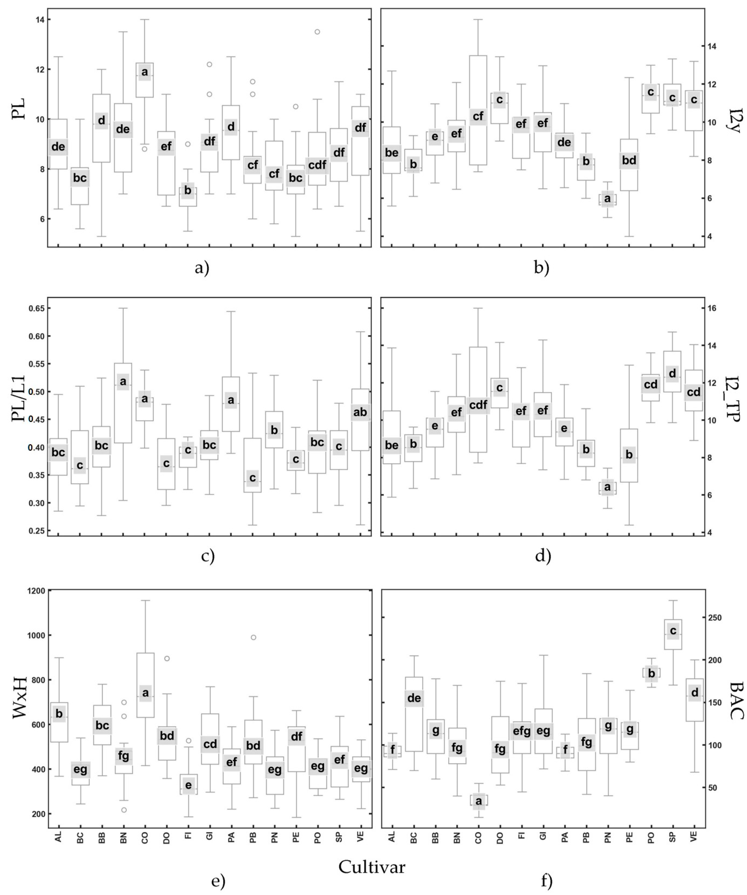
- Panel a: variable PL shows considerable variability among cultivars, with statistically significant differences evident across groups (e.g., cultivar CO differs significantly from cultivars BC and FI).
- Panel b: variable I2y show statistically significant differences for all cultivars except for SP, PO and VE, which show similar values.
- Panel c: variable PL/L1 displays a narrower range, indicating lower variability, with several cultivars sharing overlapping groups (e.g., BC, DO, PB, PE, and SP).
- Panel d: trait I2_TP reveals intermediate variability, with notable outliers in certain cultivars, such as CO and PE.
- Panel e: variable WxH demonstrates the greatest variability, as reflected by the wider interquartile ranges and the presence of several outliers, such as CO.
- Panel f: trait BAC displays smaller interquartile ranges and a more consistent pattern, indicating less variability across cultivars. Significant differences evident for some cultivar (e.g., PO, SP, and VE compared with CO).
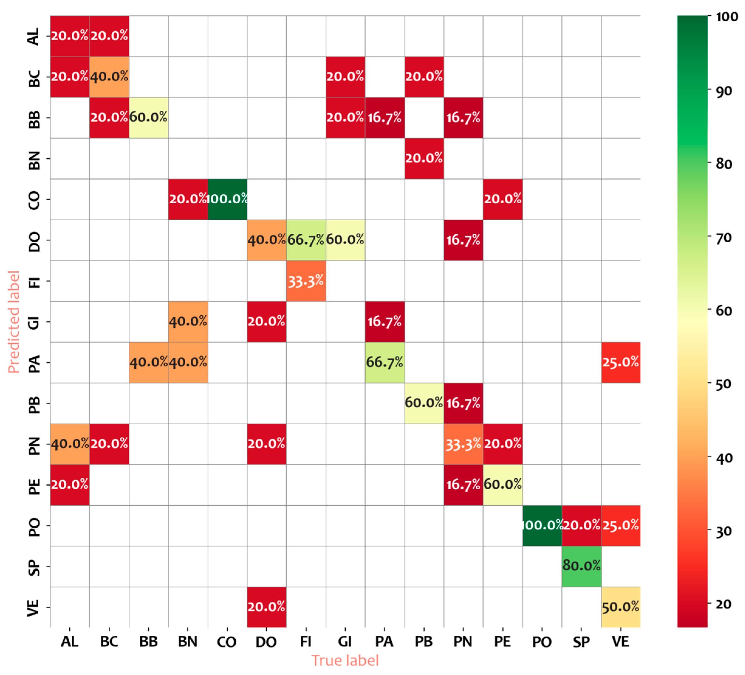
2.1.2. Cultivar Classification by Random Forest
- Class-wise Performance: Cultivars such as CO and SP show the best classification performance with high precision (0.71 and 1.00), recall (1.00), and F1-scores (0.83 and 0.89), indicating that the model accurately identifies these cultivars with few misclassifications. On the contrary, cultivars like BN and GI exhibit the poorest performance, with all metrics (precision, recall, and F1-score) at 0.00. This suggests that the classifier struggles entirely with these cultivars, likely due to class imbalance, lack of distinctive features, or other limitations in the dataset.
- Intermediate Performance: Cultivars such as PE, PO, and PB have moderate F1-scores ranging from 0.60 to 0.75. While the recall is strong for some, such as PO (0.60 precision, 1.00 recall), the precision-recall trade-off indicates room for improvement in minimizing false positives.
- Poor Recall for High Precision Cultivars: A notable case is FI, which shows perfect precision (1.00) but a recall of only 0.33, resulting in a moderate F1-score (0.50). This suggests that while the classifier is confident when it predicts FI, it fails to capture many actual instances, indicating underprediction for this class.
- Weighted Metrics: the weighted average precision, recall, and F1-score are 0.49, 0.49, and 0.47, respectively. These values reflect the overall performance across all cultivars, weighted by the number of instances in each class. The low values indicate that the classifier struggles to generalize well across multiple classes.
- Overall Accuracy: The overall accuracy of the classifier is 0.49, which is only slightly better than random chance in a binary context. This underscores the challenges the classifier faces in achieving consistent performance across cultivars.
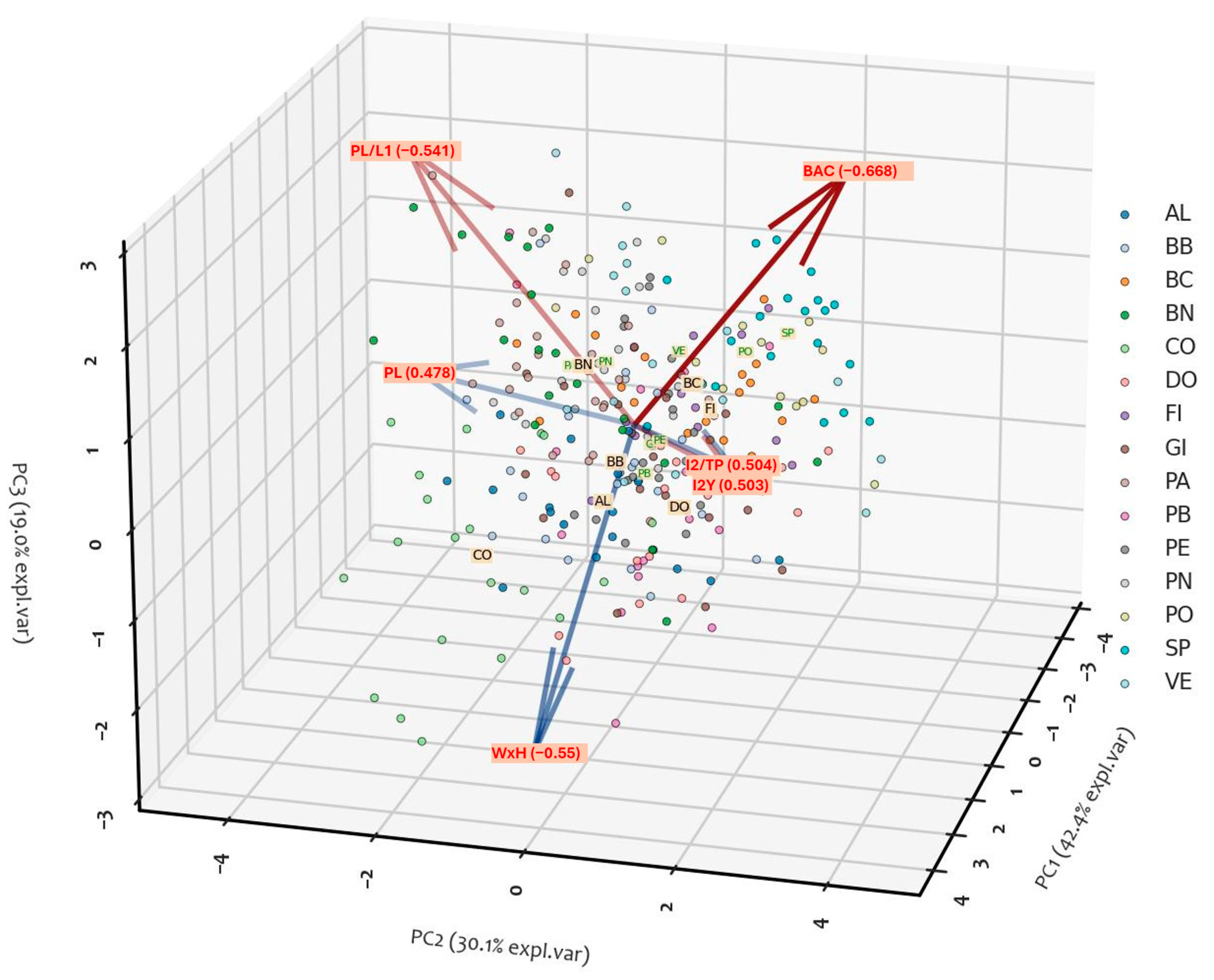
2.1.3. PCA Analysis
2.2. Trichome Analysis
3. Materials and Methods
3.1. Plant Material
3.2. Morphological Descriptors
3.3. Trichome Analysis
3.4. Statistical, PCA Analysis, and Random Forest Model
3.4.1. Trichomes
3.4.2. Morphological Variables
3.4.3. Random Forest Model
3.4.4. Software Used and Coding
4. Conclusions
Supplementary Materials
Author Contributions
Funding
Data Availability Statement
Conflicts of Interest
References
- Linné, C.V.; Salvius, L. Caroli Linnaei …Species Plantarum: Exhibentes Plantas Rite Cognitas, Ad Genera Relatas, Cum Differentiis Specificis, Nominibus Trivialibus, Synonymis Selectis, Locis Natalibus, Secundum Systema Sexuale Digestas…; Impensis Laurentii Salvii: Holmiae, Sweden, 1753. [Google Scholar]
- Langgut, D. The Core Area of Fruit-Tree Cultivation: Central Jordan Valley (Levant), ca. 7000 BP. Palynology 2024, 48, 2347905. [Google Scholar] [CrossRef]
- Langgut, D.; Garfinkel, Y. 7000-Year-Old Evidence of Fruit Tree Cultivation in the Jordan Valley, Israel. Sci. Rep. 2022, 12, 7463. [Google Scholar] [CrossRef] [PubMed]
- Zohary, D.; Hopf, M.; Weiss, E. Domestication of Plants in the Old World: The Origin and Spread of Domesticated Plants in Southwest Asia, Europe, and the Mediterranean Basin; Oxford University Press: Oxford, UK, 2012. [Google Scholar]
- Walthall, D.A. Agriculture in Magna Graecia (Iron Age to Hellenistic Period). In A Companion to Ancient Agriculture; Hollander, D., Howe, T., Eds.; Wiley: New York, NY, USA, 2020; pp. 317–341. ISBN 978-1-118-97092-8. [Google Scholar]
- Moricca, C. Sacred and Secular Aspects of Phoenicians’ Life at Motya (Sicily, Italy) Inferred by Multidisciplinary Archaeobotanical Analyses. Rendiconti Online Della Soc. Geol. Ital. 2021, 54, 2–8. [Google Scholar] [CrossRef]
- Mazzeo, A.; Magarelli, A.; Ferrara, G. The Fig (Ficus carica L.): Varietal Evolution from Asia to Puglia Region, Southeastern Italy. CABI Agric. Biosci. 2024, 5, 57. [Google Scholar]
- Food and Agriculture Organization of the United Nations FAOSTAT Statistical Database. Available online: https://www.fao.org/statistics/en (accessed on 24 November 2024).
- Desa, W.N.M.; Mohammad, M.; Fudholi, A. Review of Drying Technology of Fig. Trends Food Sci. Technol. 2019, 88, 93–103. [Google Scholar] [CrossRef]
- Ferrara, G.; Mazzeo, A.; Colasuonno, P.; Marcotuli, I. Production and Growing Regions. In The Fig: Botany, Production and Uses; CABI GB: New York, NY, USA, 2022; pp. 47–92. [Google Scholar]
- Italian Parliament Official Gazette of 21/1/2017 Gen. Series No. 17. 2017. Available online: https://www.gazzettaufficiale.it/atto/serie_generale/caricaDettaglioAtto/originario?atto.dataPubblicazioneGazzetta=2017-01-21&atto.codiceRedazionale=17A00355&elenco30giorni=false (accessed on 24 November 2024).
- Bonamici, M.; Rosselli, L.; Taccola, E. Il Santuario Dell’Acropoli Di Volterra; DISCI-Archelogia, 2017; pp. 51–74. Available online: https://www.researchgate.net/publication/320877556_Il_santuario_dell’acropoli_di_Volterra (accessed on 24 November 2024).
- Caneva, G.; Zangari, G.; Lazzara, A.; D’Amato, L.; Maras, D.F. Trees and the Significance of Sacred Grove Imagery in Etruscan Funerary Paintings at Tarquinia (Italy). Rendiconti Lincei Sci. Fis. E Nat. 2024, 35, 637–654. [Google Scholar] [CrossRef]
- Rattighieri, E.; Rinaldi, R.; Bowes, K.; Mercuri, A.M.; Bowes, K. Land Use from Seasonal Archaeological Sites: The Archaeobotanical Evidence of Small Roman Farmhouses in Cinigiano, South-Eastern Tuscany-Central Italy. Ann. Bot. 2013, 3, 207–215. [Google Scholar]
- Giachi, G.; Bettazzi, F.; Chimichi, S.; Staccioli, G. Chemical Characterisation of Degraded Wood in Ships Discovered in a Recent Excavation of the Etruscan and Roman Harbour of Pisa. J. Cult. Herit. 2003, 4, 75–83. [Google Scholar] [CrossRef]
- Mariotti Lippi, M.; Bellini, C.; Mori Secci, M.; Gonnelli, T.; Pallecchi, P. Archaeobotany in Florence (Italy): Landscape and Urban Development from the Late Roman to the Middle Ages. Plant Biosyst. Int. J. Deal. Asp. Plant Biol. 2015, 149, 216–227. [Google Scholar] [CrossRef]
- Del Riccio, A. Firenze, Università Degli Studi, Biblioteca Biomedica, Fondo Ant., MSS.R.210.2_1. Available online: https://www.internetculturale.it/it/16/search?instance=magindice&q=&qq=%28%28typeTipo%3A%22manoscritti%22%29+OR+%28typeTipo%3A%22manoscritto%22%29%29&__meta_agency=it%3A+unfi%2C+universita+degli+studi+di+firenze%2C+sistema+bibliotecario+di+ateneo&pag=8 (accessed on 24 November 2024).
- Baldini, E. Alcuni Aspetti Della Coltura Del Fico Nella Provincia Di Firenze. Riv. Ortoflorofruttic. Ital. 1953, 185–203. Available online: https://www.jstor.org/stable/42872468 (accessed on 24 November 2024).
- Targioni-Tozzetti, O. Lezioni di Agricoltura Specialmente Toscana—Tomo III.; Piatti: Firenze, Italy, 1802; Volume III. [Google Scholar]
- Gallesio, G.; Baldini, E. Il Commercio Della Frutta Negli Scritti di Giorgio Gallesio; Accademia dei Georgofili: Firenze, Italy, 2003. [Google Scholar]
- Rodolfi, M.; Ganino, T.; Chiancone, B.; Petruccelli, R. Identification and Characterization of Italian Common Figs (Ficus carica) Using Nuclear Microsatellite Markers. Genet. Resour. Crop Evol. 2018, 65, 1337–1348. [Google Scholar] [CrossRef]
- Giraldo, E.; López-Corrales, M.; Hormaza, J.I. Selection of the Most Discriminating Morphological Qualitative Variables for Characterization of Fig Germplasm. J. Am. Soc. Hortic. Sci. 2010, 135, 240–249. [Google Scholar] [CrossRef]
- Abdelkader, F.; Laiadi, Z.; Boso, S.; Santiago, J.-L.; Gago, P.; Martínez, M.-C. Algerian Fig Trees: Botanical and Morphometric Leaf Characterization. Horticulturae 2023, 9, 612. [Google Scholar] [CrossRef]
- Nuzzo, V.; Gatto, A.; Montanaro, G. Morphological Characterization of Some Local Varieties of Fig (Ficus carica L.) Cultivated in Southern Italy. Sustainability 2022, 14, 15970. [Google Scholar] [CrossRef]
- Ciarmiello, L.F.; Piccirillo, P.; Carillo, P.; De Luca, A.; Woodrow, P. Determination of the Genetic Relatedness of Fig (Ficus carica L.) Accessions Using RAPD Fingerprint and Their Agro-Morphological Characterization. S. Afr. J. Bot. 2015, 97, 40–47. [Google Scholar] [CrossRef]
- Azlah, M.A.F.; Chua, L.S.; Rahmad, F.R.; Abdullah, F.I.; Wan Alwi, S.R. Review on Techniques for Plant Leaf Classification and Recognition. Computers 2019, 8, 77. [Google Scholar] [CrossRef]
- Falaschetti, L.; Manoni, L.; Di Leo, D.; Pau, D.; Tomaselli, V.; Turchetti, C. A CNN-Based Image Detector for Plant Leaf Diseases Classification. HardwareX 2022, 12, e00363. [Google Scholar] [CrossRef] [PubMed]
- Hastie, T.; Tibshirani, R.; Friedman, J. Random Forests. In The Elements of Statistical Learning; Springer Series in Statistics; Springer: New York, NY, USA, 2009; pp. 587–604. ISBN 978-0-387-84857-0. [Google Scholar]
- Cutler, A.; Cutler, D.R.; Stevens, J.R. Random Forests. In Ensemble Machine Learning; Zhang, C., Ma, Y., Eds.; Springer: New York, NY, USA, 2012; pp. 157–175. ISBN 978-1-4419-9325-0. [Google Scholar]
- Breiman, L. Random Forest. Mach. Learn. 2001, 45, 5–32. [Google Scholar] [CrossRef]
- Ljubobratović, D.; Vuković, M.; Brkić Bakarić, M.; Jemrić, T.; Matetić, M. Utilization of Explainable Machine Learning Algorithms for Determination of Important Features in ‘Suncrest’ Peach Maturity Prediction. Electronics 2021, 10, 3115. [Google Scholar] [CrossRef]
- Ayala-Niño, D.; González-Camacho, J.M. Evaluation of Machine Learning Models to Identify Peach Varieties Based on Leaf Color. Agrociencia 2022, 56, 1–17. [Google Scholar] [CrossRef]
- Ropelewska, E.; Rutkowski, K.P. Differentiation of Peach Cultivars by Image Analysis Based on the Skin, Flesh, Stone and Seed Textures. Eur. Food Res. Technol. 2021, 247, 2371–2377. [Google Scholar] [CrossRef]
- International Plant Genetic Resources Institute (IPGRI). AA.VV Descriptors for Fig (Ficus carica L.); International Plant Genetic Resources Institute (IPGRRI): Rome, Italy, 2003. [Google Scholar]
- Descriptors for Fig: Ficus carica; IPGRI: Rome, Italy; CIHEAM: Paris, France, 2003; ISBN 978-92-9043-598-3.
- Mubo, S.A.; Adeniyi, J.A.; Adeyemi, E. A Morphometric Analysis of the Genus Ficus Linn. (Moraceae). Afr. J. Biotechnol. 2004, 3, 229–235. [Google Scholar] [CrossRef]
- Jangam, A.; Jadhav, S.; Sutar, V.; Onkar, R.; Deshmukh, S. Leaf Morphometric Studies in Some Species of Ficus L. Res. Rev. J. Bot. 2017, 6, 29–31. [Google Scholar]
- Wagner, G.; Wang, E.; Shepherd, R. New Approaches for Studying and Exploiting an Old Protuberance, the Plant Trichome. Ann. Bot. 2004, 93, 3. [Google Scholar] [CrossRef] [PubMed]
- Tattini, M.; Matteini, P.; Saracini, E.; Traversi, M.L.; Giordano, C.; Agati, G. Morphology and Biochemistry of Non-Glandular Trichomes in Cistus salvifolius L. Leaves Growing in Extreme Habitats of the Mediterranean Basin. Plant Biol. 2007, 9, 411–419. [Google Scholar] [CrossRef] [PubMed]
- Bei, Z.; Zhang, X.; Zhang, F.; Yan, X. The Response of Oxytropis aciphylla Ledeb. Leaf Interface to Water and Light in Gravel Deserts. Plants 2023, 12, 3922. [Google Scholar] [CrossRef]
- Vanhoutte, B.; Schenkels, L.; Ceusters, J.; De Proft, M.P. Water and Nutrient Uptake in Vriesea Cultivars: Trichomes vs. Roots. Environ. Exp. Bot. 2017, 136, 21–30. [Google Scholar] [CrossRef]
- Wang, D.; Liang, X.; Mofack, G.I.; Martin-Ducup, O. Individual Tree Extraction from Terrestrial Laser Scanning Data via Graph Pathing. For. Ecosyst. 2021, 8, 67. [Google Scholar] [CrossRef]
- Bickford, C.P. Ecophysiology of Leaf Trichomes. Funct. Plant Biol. 2016, 43, 807–814. [Google Scholar] [CrossRef]
- Song, J.-H.; Yang, S.; Choi, G. Taxonomic Implications of Leaf Micromorphology Using Microscopic Analysis: A Tool for Identification and Authentication of Korean Piperales. Plants 2020, 9, 566. [Google Scholar] [CrossRef] [PubMed]
- Pinto-Silva, N.P.; De Souza, K.F.; Marques Silva, O.L.; Vitarelli, N.C.; Da Paixão Noronha Pereira, A.; Soares, D.A.; Sodré, R.C.; Medeiros, D.; Caruzo, M.B.R.; Carneiro Torres, D.S.; et al. Trichomes in the Megadiverse Genus Croton (Euphorbiaceae): A Revised Classification, Identification Parameters and Standardized Terminology. Bot. J. Linn. Soc. 2023, 203, 37–49. [Google Scholar] [CrossRef]
- Giordano, C.; Maleci, L.; Agati, G.; Petruccelli, R. Ficus carica L. Leaf Anatomy: Trichomes and Solid Inclusions. Ann. Appl. Biol. 2020, 176, 47–54. [Google Scholar] [CrossRef]
- Dixon, W.J. Simplified Estimation from Censored Normal Samples. Ann. Math. Stat. 1960, 31, 385–391. [Google Scholar] [CrossRef]
- Abdi, H.; Williams, L.J. Tukey’s Honestly Significant Difference (HSD) Test. Encycl. Res. Des. 2010, 3, 1–5. [Google Scholar]
- Cohen, J. Statistical Power Analysis for the Behavioral Sciences; Cohen, J., Ed.; Academic Press: New York, NY, USA, 1977; ISBN 978-0-12-179060-8. [Google Scholar]
- Buitinck, L.; Louppe, G.; Blondel, M.; Pedregosa, F.; Mueller, A.; Grisel, O.; Niculae, V.; Prettenhofer, P.; Gramfort, A.; Grobler, J.; et al. API Design for Machine Learning Software: Experiences from the Scikit-Learn Project. In Proceedings of the ECML PKDD Workshop: Languages for Data Mining and Machine Learning, INRIA Saclay-Ile de France, Prague, Czech Republic, 23–27 September 2013; pp. 108–122. [Google Scholar]
- Pedregosa, F.; Varoquaux, G.; Gramfort, A.; Michel, V.; Thirion, B.; Grisel, O.; Blondel, M.; Prettenhofer, P.; Weiss, R.; Dubourg, V.; et al. Scikit-Learn: Machine Learning in Python. J. Mach. Learn. Res. 2011, 12, 2825–2830. [Google Scholar]
- Virtanen, P.; Gommers, R.; Oliphant, T.E.; Haberland, M.; Reddy, T.; Cournapeau, D.; Burovski, E.; Peterson, P.; Weckesser, W.; Bright, J.; et al. SciPy 1.0: Fundamental Algorithms for Scientific Computing in Python. Nat. Methods 2020, 17, 261–272. [Google Scholar] [CrossRef]
- The Pandas Development Pandas-Dev/Pandas: Pandas 2020. Available online: https://github.com/pandas-dev/pandas/blob/main/CITATION.cff (accessed on 24 November 2024).
- Jordahl, K. GeoPandas: Python Tools for Geographic Data. 2014. Available online: https://github.com/geopandas/geopandas (accessed on 24 November 2024).
- Seabold, S.; Perktold, J. Statsmodels: Econometric and Statistical Modeling with Python. In Proceedings of the 9th Python in Science Conference, Austin, TX, USA, 28–30 June 2010. [Google Scholar]
- Vallat, R. Pingouin: Statistics in Python. J. Open Source Softw. 2018, 3, 1026. [Google Scholar] [CrossRef]
- Waskom, M. Seaborn: Statistical Data Visualization. J. Open Source Softw. 2021, 6, 3021. [Google Scholar] [CrossRef]
- Hunter, J.D. Matplotlib: A 2D Graphics Environment. Comput. Sci. Eng. 2007, 9, 90–95. [Google Scholar] [CrossRef]
- Podgornik, M.; Vuk, I.; Vrhovnik, I.; Mavsar, D.B. A Survey and Morphological Evaluation of Fig (Ficus carica L.) Genetic Resources from Slovenia. Sci. Hortic. 2010, 125, 380–389. [Google Scholar] [CrossRef]
- Khadivi, A.; Mirheidari, F. Phenotypic Variability of Fig (Ficus carica L.). In Fig (Ficus carica L.): Production, Processing, and Properties; Ramadan, M.F., Ed.; Springer International Publishing: Cham, Switzerland, 2023; pp. 129–174. ISBN 978-3-031-16492-7. [Google Scholar]


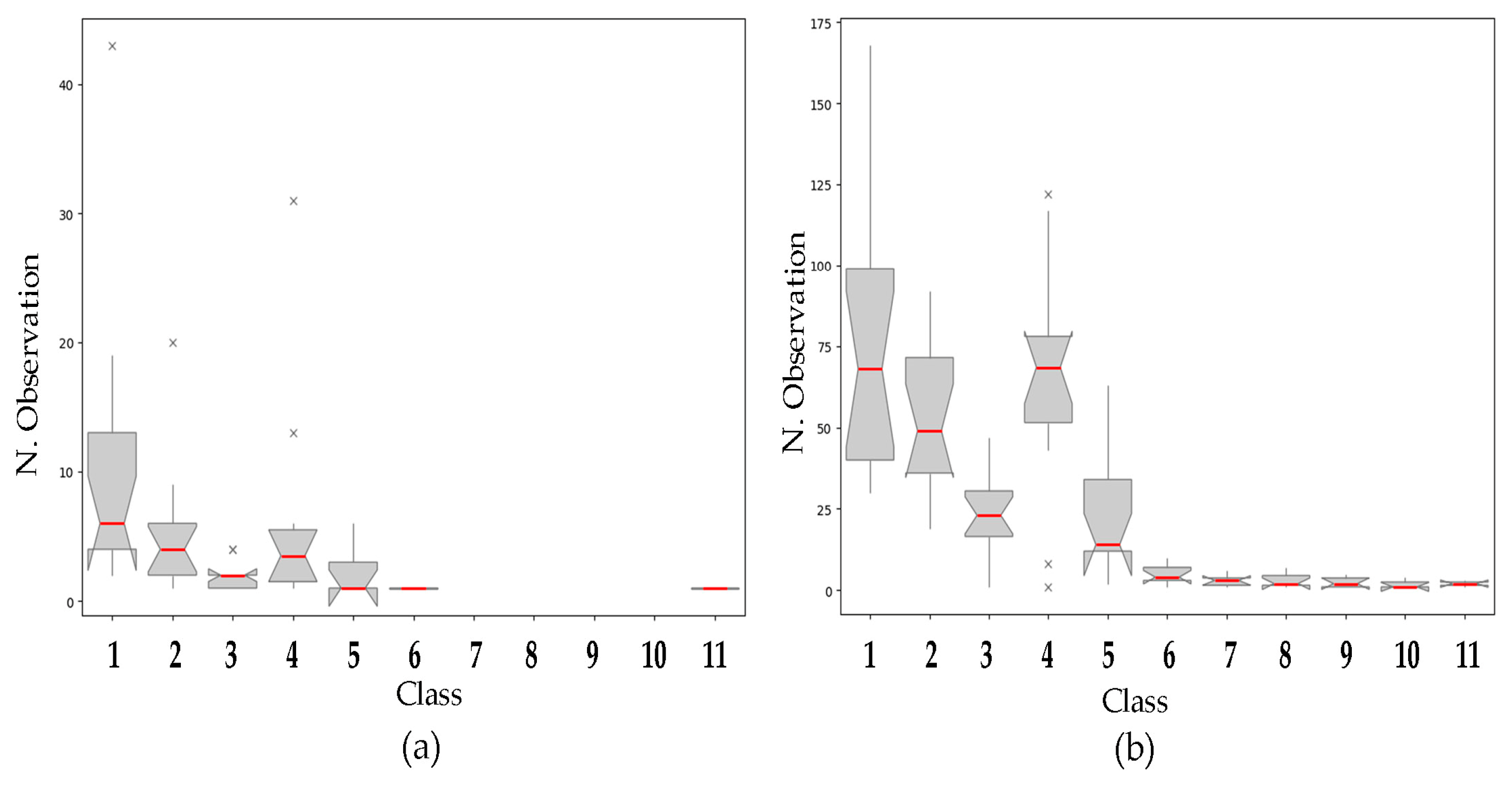
 . Class n. 1: 0.1–99 µm; class n. 2: 100–140 µm; class n. 3: 140.1–159 µm; class n. 4: 160–239 µm; class n. 5: 240–299 µm; class n. 6: 300–319 µm; class n. 7: 320–332 µm; class n. 8: 334–358 µm; class n. 9: 360–398 µm; class n. 10: 412–438 µm; class n. 11: 450–477 µm. The codes of the cultivars are reported in Table 1.
. Class n. 1: 0.1–99 µm; class n. 2: 100–140 µm; class n. 3: 140.1–159 µm; class n. 4: 160–239 µm; class n. 5: 240–299 µm; class n. 6: 300–319 µm; class n. 7: 320–332 µm; class n. 8: 334–358 µm; class n. 9: 360–398 µm; class n. 10: 412–438 µm; class n. 11: 450–477 µm. The codes of the cultivars are reported in Table 1.
. Class n. 1: 0.1–99 µm; class n. 2: 100–140 µm; class n. 3: 140.1–159 µm; class n. 4: 160–239 µm; class n. 5: 240–299 µm; class n. 6: 300–319 µm; class n. 7: 320–332 µm; class n. 8: 334–358 µm; class n. 9: 360–398 µm; class n. 10: 412–438 µm; class n. 11: 450–477 µm. The codes of the cultivars are reported in Table 1.


| Cultivar | Code | Leaf Margin | Shape of Central Lobe | Shape of Leaf Bas | Little Lobe in Central Lobe (%) | Little Lobe in Lateral Lobe (%) | N. of Lobes |
|---|---|---|---|---|---|---|---|
| ALBO | AL | crenate | lyrate- lanceolate | calcarate-cordate | 11.11 | 44.44 | 5 |
| BIANCO DI CARMIGNANO | BC | crenate | lanceolate | truncate -cordate | 31.58 | 25.00 | 3 * |
| BROGIOTTO BIANCO | BB | crenate/dentato | lanceolate | cordate- calcarate | 25.00 | 20.00 | 3 * |
| BROGIOTTO NERO | BN | crenate | lanceolate- romboidale | cordate calcarate-truncate | 15.00 | 5.00 | 3 |
| CORBO | CO | crenate | lanceolate- lyrate | calcarate | 68.42 | 55.00 | 5 |
| DOTTATO | DO | crenate | lanceolate | cordate | 65.00 | 5.00 | 3 * |
| FIORONE | FI | crenate | lanceolate | cordate | 18.18 | 100.00 | 3 |
| GIGANTE DI CARMIGNANO | GI | crenate | lanceolate | cordate-truncate | 65.00 | 31.58 | 3 * |
| PARADISO | PA | crenate | lanceolate | calcarate | 20.83 | 8.70 | 3 |
| PECCIOLOBIANCO | PB | undulate/crenate | lanceolate | cordate-calcarate | 30.00 | 25.00 | 3 * |
| PECCIOLO NERO | PN | crenate | linear | cordate-calcarate | 65.00 | 50.00 | 5 |
| PERTICONE | PE | crenate | lanceolate- spatulate | cordate | 45.45 | 59.09 | 5 |
| PORTOGALLO | PO | crenate | lanceolate | truncate | 82.35 | 78.57 | 3 |
| SAN PIERO | SP | crenate | lanceolate | decurrente | 45.00 | 15.00 | 3 |
| VERDINO | VE | crenate | lanceolate | truncate | 22.22 | 33.33 | 3 |
| Descriptor | No Sample | Mean | Standard Error | Standard Deviation | Median | Min | Max | 1st Quartile | 3th Quartile | CV |
|---|---|---|---|---|---|---|---|---|---|---|
| L3y (cm) | 134 | 2.7 | 0.2 | 1.9 | 2.5 | −3.8 | 9.8 | 1.5 | 3.8 | 72.5% |
| BAC (°) | 287 | 117.8 | 3.1 | 52.7 | 110.0 | 15.2 | 270.0 | 85.0 | 157.5 | 44.6% |
| I3y (cm) | 134 | 3.3 | 0.1 | 1.2 | 3.3 | 0.5 | 6.5 | 2.4 | 4.0 | 36.6% |
| WxH (cm2) | 287 | 483.6 | 9.8 | 165.2 | 460.0 | 185.0 | 1156.0 | 371.9 | 567.8 | 34.1% |
| I2x (cm) | 286 | 3.3 | 0.1 | 1.0 | 3.2 | 1.5 | 6.8 | 2.5 | 4.0 | 31.5% |
| I3x (cm) | 134 | 6.5 | 0.1 | 1.6 | 6.4 | 2.6 | 10.5 | 5.5 | 7.5 | 24.2% |
| L3 (cm) | 134 | 10.5 | 0.2 | 2.5 | 10.4 | 5.5 | 17.7 | 8.5 | 12.5 | 23.8% |
| I2_TP (cm) | 287 | 9.8 | 0.1 | 2.3 | 9.8 | 4.4 | 16.0 | 8.2 | 11.5 | 23.5% |
| I2y (cm) | 286 | 9.2 | 0.1 | 2.2 | 9.2 | 4.0 | 15.4 | 7.5 | 11.0 | 23.5% |
| L3x (cm) | 134 | 10.0 | 0.2 | 2.3 | 10.0 | 5.2 | 15.1 | 8.0 | 11.8 | 23.0% |
| I2/L2 | 287 | 0.6 | 0.0 | 0.1 | 0.6 | 0.3 | 0.9 | 0.5 | 0.7 | 22.4% |
| I3_TP (cm) | 134 | 7.4 | 0.1 | 1.6 | 7.4 | 3.5 | 11.3 | 6.2 | 8.8 | 22.1% |
| CLL (cm) | 287 | 12.0 | 0.2 | 2.6 | 12.0 | 6.0 | 19.3 | 10.0 | 14.0 | 21.8% |
| Pl Ø (cm) | 287 | 0.6 | 0.0 | 0.1 | 0.5 | 0.3 | 1.0 | 0.5 | 0.6 | 21.3% |
| PL (cm) | 287 | 8.8 | 0.1 | 1.8 | 8.5 | 5.3 | 14.0 | 7.5 | 10.0 | 21.0% |
| PL/H | 287 | 0.4 | 0.0 | 0.1 | 0.4 | 0.2 | 0.6 | 0.3 | 0.4 | 19.1% |
| L2y (cm) | 287 | 13.5 | 0.2 | 2.6 | 13.3 | 7.0 | 20.8 | 11.7 | 15.2 | 19.0% |
| L2x (cm) | 287 | 9.1 | 0.1 | 1.6 | 9.0 | 5.5 | 13.5 | 8.0 | 10.0 | 18.1% |
| PL/L1 | 287 | 0.4 | 0.0 | 0.1 | 0.4 | 0.3 | 0.7 | 0.4 | 0.5 | 18.1% |
| W (cm) | 287 | 20.3 | 0.2 | 3.6 | 20.0 | 12.5 | 33.3 | 17.9 | 22.5 | 17.8% |
| α (°) | 287 | 39.8 | 0.4 | 7.1 | 40.0 | 20.0 | 62.1 | 35.0 | 45.0 | 17.7% |
| L3/L1 | 134 | 0.5 | 0.0 | 0.1 | 0.5 | 0.3 | 0.7 | 0.4 | 0.5 | 17.3% |
| Zx (cm) | 287 | 4.7 | 0.0 | 0.8 | 4.6 | 2.5 | 7.0 | 4.0 | 5.0 | 17.3% |
| I3/L3 | 134 | 0.7 | 0.0 | 0.1 | 0.7 | 0.5 | 1.0 | 0.6 | 0.8 | 17.3% |
| H (cm) | 287 | 23.3 | 0.2 | 3.9 | 23.0 | 15.0 | 37.0 | 20.5 | 25.6 | 16.9% |
| L2_TP (cm) | 287 | 16.4 | 0.2 | 2.7 | 16.3 | 9.7 | 24.1 | 14.4 | 18.2 | 16.6% |
| R (cm) | 136 | 0.6 | 0.0 | 0.1 | 0.6 | 0.4 | 0.8 | 0.5 | 0.7 | 16.5% |
| Zy (cm) | 287 | 14.1 | 0.1 | 2.3 | 13.9 | 7.7 | 20.0 | 12.5 | 15.6 | 16.3% |
| CLL/H | 276 | 0.5 | 0.0 | 0.1 | 0.5 | 0.3 | 0.8 | 0.5 | 0.6 | 16.2% |
| Z_TP (cm) | 287 | 14.9 | 0.1 | 2.3 | 14.6 | 9.3 | 20.8 | 13.2 | 16.5 | 15.4% |
| L1 (cm) | 287 | 21.3 | 0.2 | 3.0 | 21.3 | 14.2 | 29.0 | 19.2 | 23.1 | 14.1% |
| β (°) | 133 | 42.3 | 0.5 | 5.3 | 42.0 | 30.0 | 57.6 | 40.0 | 45.0 | 12.5% |
| L2/L1 | 287 | 0.8 | 0.0 | 0.1 | 0.8 | 0.5 | 1.0 | 0.7 | 0.8 | 8.4% |
| Descriptor | BC | BB | BN | DO | FI | GI | PA | PO | PB | SP | VE |
|---|---|---|---|---|---|---|---|---|---|---|---|
| PL (cm) | 7.44 ± 1.2 b | 9.57 ± 1.7 a | 9.54 ± 1.9 a | 8.52 ± 1.5 a–c | 6.95 ± 1.5 c | 8.74 ± 1.0 a–c | 9.49 ± 1.5 a | 8.52 ± 1.9 a–c | 8.02 ± 1.4 a–c | 8.62 ± 1.4 a–c | 8.93 ± 1.8 ab |
| PL Ø (cm) | 0.55 ± 0.1 ns | 0.51 ± 0.06 ns | 0.53 ± 0.07 ns | 0.64 ± 0.1 ns | 0.49 ± 0.1 ns | 0.54 ± 0.09 ns | 0.60 ± 0.1 ns | 0.50 ± 0.1 ns | 0.70 ± 0.08 ns | 0.51 ± 0.09 ns | 0.47 ± 0.08 ns |
| L1 (cm) | 19.6 ± 2.5 c–e | 24.0 ± 2.2 a | 19.8 ± 2.8 c–e | 22.8 ± 1.8 ab | 18.4 ± 1.9 e | 21.8 ± 2.7 a–d | 19.6 ± 2.3 de | 20.7 ± 1.8 b–e | 21.6 ± 2.9 a–d | 22.1 ± 2.3 a–c | 20.1 ± 2.0 c–e |
| I2 x (cm) | 2.83 ± 0.8 c | 2.89 ± 0.4 c | 4.39 ± 1.1 a | 3.88 ± 0.6 ab | 3.25 ± 0.8 bc | 3.42 ± 1.1 bc | 3.31 ± 0.7 bc | 3.27 ± 0.4 bc | 3.26 ± 1.2 bc | 3.98 ± 1.1 ab | 4.05 ± 0.9 ab |
| I2 y (cm) | 7.76 ± 1.1 f | 8.94 ± 1.2 d–f | 9.38 ± 2.1 c–e | 10.9 ± 1.3 ab | 9.37 ± 1.5 c–f | 9.75 ± 2.3 b–d | 8.82 ± 1.6 d–f | 11.3 ± 1.1 ab | 7.91 ± 1.3 ef | 11.4 ± 1.3 a | 10.9 ± 1.0 a–c |
| I2_TP (cm) | 8.30 ± 1.1 d | 9.40 ± 1.2 cd | 10.4 ± 2.1 bc | 11.6 ± 1.3 ab | 9.93 ± 1.6 b–d | 10.4 ± 2.4 bc | 9.43 ± 1.7 cd | 11.8 ± 1.1 ab | 8.61 ± 1.5 d | 12.1 ± 1.5 a | 11.6 ± 1.5 ab |
| L2 x (cm) | 8.69 ± 1.4 b–d | 10.5 ± 1.2 a | 9.26 ± 1.2 a–d | 9.94 ± 1.2 ab | 7.52 ± 0.9 d | 9.39 ± 1.7 a–c | 8.21 ± 1.1 cd | 7.89 ± 1.3 cd | 10.5 ± 1.4 a | 8.65 ± 1.6 b–d | 8.04 ± 1.2 cd |
| L2 y (cm) | 11.6 ± 2.2 c | 15.0 ± 2.0 ab | 12.3 ± 2.0 c | 15.9 ± 1.8 a | 11.6 ± 1.7 c | 12.3 ± 2.2 c | 12.3 ± 2.0 c | 13.7 ± 1.8 a–c | 12.7 ± 2.6 bc | 13.4 ± 1.7 bc | 13.0 ± 1.1 bc |
| L2_TP (cm) | 14.5 ± 2.3 c | 18.3 ± 2.1 ab | 15.5 ± 2.2 c | 18.8 ± 1.9 a | 13.8 ± 1.8 c | 15.7 ± 2.9 c | 14.8 ± 2.2 c | 15.9 ± 1.9 bc | 16.6 ± 3.0 a–c | 15.9 ± 2.1 bc | 15.3 ± 1.8 c |
| Z x (cm) | 4.27 ± 0.6 b | 5.11 ± 0.7 a | 5.09 ± 0.6 a | 4.31 ± 0.5 b | 5.05 ± 0.6 ab | 4.69 ± 0.9 ab | 4.37 ± 0.7 b | 4.48 ± 0.7 ab | 4.89 ± 0.6 ab | 4.88 ± 0.4 ab | 4.73 ± 0.7 ab |
| Zy (cm) | 14.2.3 ± 2.4 ab | 13.5 ± 1.6 ab | 14.5 ± 2.3 ab | 13.4 ± 2.0 ab | 15.7 ± 1.8 a | 13.4 ± 2.4 ab | 13.0 ± 2.44 b | 13.0 ± 1.2 ab | 12.5 ± 2.7 b | 14.2 ± 0.8 ab | 11.1 ± 1.9 b |
| Z_TP (cm) | 14.4 ± 3.2 a–c | 14.5 ± 1.6 | 15.4 ± 2.1 ab | 14.1 ± 1.9 a–c | 16.5 ± 1.7 a | 14.2 ± 2.6 a–c | 13.7 ± 1.7 bc | 14.4 ± 1.2 a–c | 13.0 ± 3.2 c | 15.0 ± 2.1 a–c | 13.9 ± 1.8 a–c |
| CLL (cm) | 11.8 ± 2.1 c | 15.1 ± 1.3 a | 10.4 ± 2.2 cd | 11.8 ± 1.7 c | 8.99 ± 1.1 d | 12.1 ± 1.9 bc | 10.8 ± 1.4 cd | 9.46 ± 1.4 d | 13.7 ± 2.6 ab | 10.8 ± 1.6 cd | 9.22 ± 1.8 d |
| W (cm) | 18.3 ± 1.9 cd | 22.7 ± 3.4 a | 19.3 ± 2.6 b–d | 21.5 ± 3.2 a–c | 16.9 ± 2.5 d | 21.7 ± 3.4 ab | 18.6 ± 2.5 cd | 18.3 ± 2.1 d | 21.6 ± 3.2 a–c | 19.3 ± 3.0 b–d | 17.8 ± 3.3 d |
| H (cm) | 21.2 ± 2.7 bc | 25.5 ± 3.5 a | 22.0 ± 2.9 bc | 25.6 ± 3.0 a | 19.7 ± 3.1 c | 23.7 ± 3.0 ab | 21.7 ± 2.8 bc | 21.1 ± 2.0 bc | 23.9 ± 4.0 ab | 22.6 ± 2.4 a–c | 21.4 ± 2.6 bc |
| BAC (°) | 140.5 ± 45 c | 113.6 ± 36 ef | 100.0 ± 37 cd | 98.7 ± 36 d | 110.4 ± 42 ef | 120.2 ± 37 cd | 91.4 ± 18 d | 183.3 ± 17 b | 103.1 ± 25 d | 226.1 ± 32 a | 145.8 ± 39 bc |
| α (°) | 40.1 ± 4.1 bc | 41.3 ± 4.2 bc | 41.9 ± 6.7 b | 36.6 ± 4.3 bc | 38.4 ± 6.2 b–d | 42.5 ± 7.5 b | 39.6 ± 4.7 bc | 31.4 ± 3.1 de | 49.4 ± 6.3 a | 29.0 ± 6.4 e | 36.0 ± 5.2 cd |
| CLL/H | 0.56 ± 0.06 ab | 0.60 ± 0.06 a | 0.47 ± 0.07 cd | 0.46 ± 0.05 cd | 0.46 ± 0.05 cd | 0.51 ± 0.07 bc | 0.50 ± 0.05 bc | 0.45 ± 0.04 cd | 0.57 ± 0.07 a | 0.48 ± 0.04 cd | 0.43 ± 0.07 d |
| PL/H | 0.35 ± 0.05 bc | 0.38 ± 0.08 a | 0.44 ± 0.09 a | 0.32 ± 0.04 c | 0.35 ± 0.03 a–c | 0.37 ± 0.07 a–c | 0.44 ± 0.07 a | 0.40 ± 0.08 a–c | 0.35 ± 0.1 bc | 0.38 ± 0.04 a–c | 0.42 ± 0.09 ab |
| WxH (cm2) | 396.2 ± 82 de | 580.6 ± 122 a | 433.9 ± 95 c–e | 558.9 ± 124 ab | 338.3 ± 91 e | 522.3 ± 141 a–d | 410.5 ± 103 c–e | 390.8 ± 103 c–e | 527.5 ± 147 a–c | 442.4 ± 112 b–e | 388.5 ± 86 e |
| PL/L1 | 0.38 ± 0.07 b | 0.39 ± 0.07 b | 0.48 ± 0.1 a | 0.37 ± 0.05 b | 0.37 ± 0.03 b | 0.40 ± 0.08 b | 0.48 ± 0.07 a | 0.41 ± 0.09 ab | 0.38 ± 0.1 b | 0.39 ± 0.05 b | 0.44 ± 0.09 ab |
| L2/L1 | 0.74 ± 0.06 b | 0.76 ± 0.04 ab | 0.78 ± 0.08 ab | 0.82 ± 0.04 a | 0.75 ± 0.04 ab | 0.72 ± 0.08 b | 0.76 ± 0.09 ab | 0.76 ± 0.06 ab | 0.77 ± 0.09 ab | 0.72 ± 0.05 b | 0.76 ± 0.05 ab |
| I2/L2 | 0.58 ± 0.1 d–f | 0.51 ± 0.04 f | 0.67 ± 0.1 a–d | 0.62 ± 0.06 c–e | 0.72 ± 0.08 a–c | 0.66 ± 0.1 a–d | 0.64 ± 0.1 b–d | 0.74 ± 0.08 ab | 0.52 ± 0.08 ef | 0.76 ± 0.08 a | 0.77 ± 0.1 a |
| Descriptor | AL | CO | PN | PE |
|---|---|---|---|---|
| PL (cm) | 9.07 ± 1.7 b | 11.6 ± 1.6 a | 8.01 ± 1.3 bc | 7.58 ± 1.3 c |
| PL Ø (cm) | 0.70 ± 0.09 a | 0.72 ± 0.13 a | 0.46 ± 0.07 b | 0.47 ± 0.09 b |
| L1 (cm) | 23.1 ± 2.4 a | 24.9 ± 2.6 a | 18.9 ± 2.6 b | 20.3 ± 2.8 b |
| I2x (cm) | 3.29 ± 1.5 a | 3.40 ± 0.9 a | 2.21 ± 0.5 b | 2.41 ± 0.7 b |
| I2y (cm) | 8.68 ± 1.9 ab | 10.5 ± 2.9 a | 5.91 ± 0.64 c | 7.82 ± 2.1 b |
| I2_TP (cm) | 9.32 ± 1.2 ab | 12.0 ± 3.0 a | 6.32 ± 0.7 c | 8.21 ± 2.1 b |
| L2x (cm) | 9.34 ± 1.89 ab | 10.7 ± 1.7 a | 8.43 ± 1.3 b | 8.56 ± 1.4 b |
| L2y (cm) | 14.3 ± 3.7 ab | 16.4 ± 2.5 a | 12.9 ± 2.8 b | 13.9 ± 2.7 b |
| L2 _TP (cm) | 17.5 ± 2.8 b | 19.6 ± 2.5 a | 15.4 ± 2.1 b | 16.4 ± 2.9 b |
| I3x (cm) | 7.31 ± 1.6 b | 8.01 ± 1.0 a | 4.89 ± 0.9 d | 5.95 ± 1.2 c |
| I3y (cm) | 3.21 ± 1.8 b | 3.60 ± 0.6 ab | 2.88 ± 0.7 b | 4.28 ± 1.2 a |
| I3_TP (cm) | 8.18 ± 1.6 ab | 8.86 ± 0.9 a | 5.71 ± 1.0 c | 7.37 ± 1.5 b |
| L3x (cm) | 10.9 ± 2.4 ab | 12.2 ± 1.7 a | 9.31 ± 1.5 b | 10.9 ± 2.2 ab |
| L3y (cm) | 2.76 ± 3.9 ab | 2.95 ± 1.3 ab | 2.88 ± 1.0 ab | 4.12 ± 1.6 a |
| L3_TP (cm) | 11.4 ± 2.2 ab | 12.6 ± 1.8 a | 9.9 ± 1.6 b | 11.7 ± 2.4 ab |
| Zx (cm) | 4.79 ± 1.4 a | 5.17 ± 0.8 a | 3.81 ± 0.7 b | 4.46 ± 0.5 ab |
| Zy (cm) | 15.1 ± 2.7 ab | 16.3 ± 2.3 a | 13.7 ± 2.0 b | 14.0 ± 1.9 b |
| Z_TP (cm) | 16.1 ± 2.5 ab | 17.1 ± 2.2 a | 14.2 ± 1.9 b | 14.9 ± 1.9 b |
| CLL (cm) | 14.3 ± 2.4 ab | 14.4 ± 2.4 a | 12.9 ± 2.3 ab | 12.5 ± 2.0 b |
| W (cm) | 23.7 ± 3.2 ab | 24.6 ± 4.4 a | 18.5 ± 2.5 c | 20.7 ± 3.7 bc |
| H (cm) | 26.1 ± 2.7 b | 30.5 ± 3.9 a | 20.5 ± 2.7 d | 22.4 ± 3.3 cd |
| BAC (°) | 91.5 ± 13 b | 34.5 ± 12.8 c | 113.4 ± 37 a | 114.8 ± 23 a |
| α (°) | 44.1 ± 8.0 ab | 44.6 ± 4.0 a | 39.7 ± 5.3 bc | 37.9 ± 4.5 c |
| β (°) | 41.4 ± 4.0 bc | 45.4 ± 2.3 a | 42.0 ± 5.2 ab | 37.5 ± 4.1 c |
| CLL/H | 0.56 ± 0.08 b | 0.48 ± 0.08 c | 0.63 ± 0.05 a | 0.56 ± 0.07 b |
| PL/H | 0.35 ± 0.05 b | 0.35 ± 0.07 b | 0.39 ± 0.05 a | 0.34 ± 0.04 b |
| WxH (cm2) | 623.6 ± 136 a | 760.2 ± 223 a | 385.9 ± 116 b | 478.9 ± 145 b |
| PL/L1 | 0.39 ± 0.06 b | 0.50 ± 0.09 a | 0.43 ± 0.05 ab | 0.38 ± 0.04 b |
| L2/L1 | 0.75 ± 0.13 ns | 0.79 ± 0.07 ns | 0.82 ± 0.06 ns | 0.81 ± 0.07 ns |
| L3/L1 | 0.50 ± 0.21 b | 0.51 ± 0.23 b | 0.52 ± 0.17 ab | 0.58 ± 0.06 a |
| I2/L2 | 0.56 ± 0.17 a | 0.56 ± 0.13 a | 0.41 ± 0.04 b | 0.50 ± 0.06 ab |
| I3/L3 | 0.72 ± 0.04 a | 0.71 ± 0.09 a | 0.59 ± 0.05 b | 0.64 ± 0.06 ab |
| R | 0.69 ± 0.19 a | 0.62 ± 0.10 ab | 0.48 ± 0.05 c | 0.55 ± 0.06 bc |
| T | p-val | CI95% | Effect Size | BF10 | Power | Class Choen | |||
|---|---|---|---|---|---|---|---|---|---|
| High Effect Size | BAC | CO||SP | −25.5 | 1.59 × 1025 | [−209.54 −178.75] | 8.07 | 9.91 × 10²¹ | 1 | Huge |
| CO||PO | −34.5 | 3.00 × 1025 | [−158.07 −140.4] | 11.90 | 1.83 × 10²³ | 1 | Huge | ||
| PA||PO | −21.2 | 4.05 × 10²⁰ | [−101.3 −83.52] | 6.80 | 3.01 × 10¹⁸ | 1 | Huge | ||
| I2_TP | PN||SP | −17.5 | 8.91 × 10²⁰ | [−6.9 −5.47] | 5.53 | 2.72 × 10¹⁶ | 1 | Huge | |
| DO||PN | 16.4 | 8.14 × 10¹⁹ | [4.64 5.95] | 5.18 | 3.23 × 10¹⁵ | 1 | Huge | ||
| PN||PO | −17.0 | 3.63 × 10¹³ | [−6.09 −4.76] | 6.47 | 2.02 × 10¹⁴ | 1 | Huge | ||
| I2y | PN||SP | −19.6 | 1.95 × 10²¹ | [−6.01 −4.88] | 6.19 | 1.09 × 10¹⁸ | 1 | Huge | |
| DO||PN | 16.1 | 1.47 × 10¹⁸ | [4.43 5.7] | 5.09 | 1.82 × 10¹⁵ | 1 | Huge | ||
| PB||SP | −10.7 | 5.37 × 10¹³ | [−4.26 −2.91] | 3.38 | 8.62 × 10⁹ | 1 | Huge | ||
| PL | BC||CO | −9.0 | 5.33 × 10¹¹ | [−5.05 −3.2] | 2.86 | 1.11 × 10⁸ | 1 | Huge | |
| CO||FI | 9.9 | 8.65 × 10¹¹ | [3.66 5.56] | 3.22 | 6.88 × 10⁷ | 1 | Huge | ||
| CO||PE | 8.7 | 1.93 × 10¹⁰ | [3.06 4.91] | 2.72 | 7.26 × 10⁷ | 1 | Huge | ||
| PL_L1 | CO||PE | 7.5 | 4.9 × 10⁹ | [0.06 0.11] | 2.34 | 2.16 × 10⁶ | 1 | Huge | |
| PA||PE | 7.1 | 1.95 × 10⁸ | [0.07 0.13] | 2.05 | 1.03 × 10⁶ | 1 | Huge | ||
| DO||PA | −6.2 | 2.13 × 10⁷ | [−0.14 −0.07] | 1.86 | 5.24 × 10⁴ | 1 | Very large | ||
| WxH | BC||CO | −6.9 | 3.0 × 10⁸ | [−479.15 −262.56] | 2.19 | 3.02 × 10⁵ | 1 | Huge | |
| CO||PN | 6.7 | 6.02 × 10⁸ | [261.43 487.17] | 2.12 | 1.61 × 10⁵ | 1 | Huge | ||
| CO||FI | 7.2 | 7.28 × 10⁸ | [301.84 542.02] | 2.22 | 1.38 × 10⁵ | 1 | Huge | ||
| Low Effect Size | BAC | BN||DO | 0.1 | 0.92 | [−21.5 23.82] | 0.03 | 0.31 | 0.0512 | Very small |
| AL||PA | 0.0 | 0.96 | [−8.45 8.87] | 0.01 | 0.306 | 0.0503 | Very small | ||
| BB||PN | 0.0 | 1.00 | [−22.4 22.35] | 0.00 | 0.309 | 0.0500 | Negligible | ||
| I2_TP | BC||PE | 0.2 | 0.81 | [−0.96 1.21] | 0.07 | 0.31 | 0.0558 | Very small | |
| BB||PA | 0.0 | 0.97 | [−0.81 0.78] | 0.01 | 0.299 | 0.0502 | Very small | ||
| DO||VE | 0.0 | 0.99 | [−0.92 0.94] | 0.01 | 0.315 | 0.0500 | Negligible | ||
| I2y | BC||PB | 0.1 | 0.93 | [−0.63 0.69] | 0.03 | 0.31 | 0.0509 | Very small | |
| PB||PE | 0.0 | 0.97 | [−1.09 1.04] | 0.01 | 0.304 | 0.0502 | Very small | ||
| BC||PE | 0.0 | 0.99 | [−1.05 1.07] | 0.00 | 0.303 | 0.0500 | Negligible | ||
| PL | BB||BN | 0.1 | 0.96 | [−1.16 1.22] | 0.02 | 0.309 | 0.0503 | Very small | |
| PB||PN | 0.0 | 0.99 | [−0.86 0.87] | 0.00 | 0.309 | 0.0500 | Negligible | ||
| DO||PO | 0.0 | 1.00 | [−1.29 1.29] | 0.00 | 0.333 | 0.0500 | Negligible | ||
| PL_L1 | BB||GI | −0.1 | 0.92 | [−0.04 0.04] | 0.03 | 0.31 | 0.0510 | Very small | |
| FI||PE | 0.1 | 0.94 | [−0.02 0.03] | 0.03 | 0.348 | 0.0505 | Very small | ||
| AL||SP | 0.1 | 0.94 | [−0.03 0.04] | 0.02 | 0.316 | 0.0506 | Very small | ||
| WxH | PO||VE | 0.1 | 0.94 | [−57.68 62.31] | 0.03 | 0.339 | 0.0507 | Very small | |
| BC||PO | 0.0 | 0.96 | [−59.82 57.02] | 0.02 | 0.333 | 0.0503 | Very small | ||
| BC||VE | 0.0 | 0.97 | [−55.73 57.56] | 0.01 | 0.315 | 0.0501 | Very small |
| Cultivars | Precision | Recall | F1-Score |
|---|---|---|---|
| AL | 0.50 | 0.20 | 0.29 |
| BC | 0.40 | 0.40 | 0.40 |
| BB | 0.43 | 0.60 | 0.50 |
| BN | 0.00 | 0.00 | 0.00 |
| CO | 0.71 | 1.00 | 0.83 |
| DO | 0.25 | 0.40 | 0.31 |
| FI | 1.00 | 0.33 | 0.50 |
| GI | 0.00 | 0.00 | 0.00 |
| PA | 0.44 | 0.67 | 0.53 |
| PB | 0.75 | 0.60 | 0.67 |
| PN | 0.29 | 0.33 | 0.31 |
| PE | 0.60 | 0.60 | 0.60 |
| PO | 0.60 | 1.00 | 0.75 |
| SP | 1.00 | 0.80 | 0.89 |
| VE | 0.67 | 0.50 | 0.57 |
| weighted average | 0.49 | 0.49 | 0.47 |
| accuracy | 0.49 | ||
| Trait | PC1 | PC2 | PC3 |
|---|---|---|---|
| WxH | 0.45 | −0.12 | −0.55 |
| PL | 0.48 | −0.39 | 0.24 |
| I2_TP | 0.50 | 0.41 | 0.11 |
| I2y | 0.51 | 0.41 | 0.09 |
| PL_L1 | 0.19 | −0.51 | 0.60 |
| BAC | −0.16 | 0.49 | 0.51 |
| Eingen Values | 2.55 | 1.8 | 1.14 |
| % of variance | 42.4 | 30.1 | 19 |
| Cumulative variance (%) | 42.4 | 72.5 | 91.5 |
| Trichomes Density (mm2) | ||
|---|---|---|
| Cv | Upper Epidermis | Lower Epidermis |
| AL | 26.3 ± 3.26 a | 48.5 ± 2.38 f |
| BB | 2.02 ± 0.77 ef | 71.5 ± 2.65 b |
| BC | 7.52 ± 1.5 b | 64.7 ± 2.78 c |
| BN | 3.50 ± 0.51 d–f | 64.5 ± 2.88 c |
| CO | 4.25 ± 035 c–f | 32.2 ± 2.18 h |
| DO | 7.48 ± 1.02 bc | 63.2 ± 1.90 c |
| FI | 5.02 ± 0.76 b–e | 23.2 ± 2.91 i |
| GI | 2.04 ± 0.89 ef | 54.2 ± 2.65 ef |
| PA | 3.26 ± 0.46 d–f | 93.8 ± 1.79 a |
| PB | 2.50 ± 0.35 d–f | 77.0 ± 1.86 b |
| PE | 5.53 ± 0.58 b–d | 87.5 ± 1.10 a |
| PN | 3.01 ± 0.36 d–f | 55.8 ± 1.56 de |
| PO | 3.02 ± 0.32 d–f | 61.5 ± 2.41 cd |
| SP | 2.76 ± 0.28 d–f | 39.7 ± 0.68 g |
| VE | 1.02 ± 0.12 f | 48.2 ± 1.14 f |
| Abbreviation | Description | Units |
|---|---|---|
| H | Lamina length | cm |
| W | Lamina width | cm |
| WxH | Area: leaf length × width | cm2 |
| PL | Petiole length | cm |
| PLØ | Petiole diameter | cm |
| CLL | Length of the central lobe | cm |
| BAC | Petiole sinus: angle between left and right basal lobe | ° |
| α | Angle between L1 and L2 | ° |
| β | Angle between L2 and L3; | ° |
| Z_TP | Central lobe maximum width calculated using the Pythagorean Theorem applied to Zx; Zy | cm |
| Zx | x coordinate of the point Z on the Cartesian plane | cm |
| Zy | y coordinate of the point Z on the Cartesian plane | cm |
| L1 | Apex of the central lobe, coincides with L1y | cm |
| L2_TP | Apex of the secondary lobe calculated using the Pythagorean Theorem applied to Lx and Ly | cm |
| L2x | x coordinate of the point L2 on the Cartesian plane | cm |
| L2y | y coordinate of the point L2 on the Cartesian plane | cm |
| I2_TP | Sinus 2 calculated using the Pythagorean Theorem applied to I2x; I2y | cm |
| I2x | x coordinate of the point I2 on the Cartesian plane | cm |
| I2y | y coordinate of the point I2 on the Cartesian plane | cm |
| L3_TP | Apex of the tertiary lobe calculated using the Pythagorean Theorem applied to L3x; L3y | cm |
| L3x | x coordinate of the point L3 on the Cartesian plane | cm |
| L3y | y coordinate of the point L3 on the Cartesian plane | cm |
| I3_TP | Sinus 3 calculated using the Pythagorean Theorem applied to I3x; I3Y | cm |
| I3x | x coordinate of the point I3 on the Cartesian plane | cm |
| I3y | y coordinate of the point I3 on the Cartesian plane | cm |
| I2/L2 | Ratio between sinus 2 (I2_TP) and apex of secondary lobe (L2_TP) | |
| L2/L1 | Ratio between apex of secondary lobe (L2_TP) and apex of central lobe (L1) | |
| I3/L3 | Ratio between sinus 3 (I3_TP) and apex of tertiary lobe (L3_TP) | |
| R | (I2_TP + I3_TP)/(L2_TP + L3_TP) | |
| PL/H | Ratio between petiole length and lamina length | |
| PL/L1 | Ratio between petiole length and apex of central lobe | |
| CLL/H | Ratio between central lobe length and lamina length |
Disclaimer/Publisher’s Note: The statements, opinions and data contained in all publications are solely those of the individual author(s) and contributor(s) and not of MDPI and/or the editor(s). MDPI and/or the editor(s) disclaim responsibility for any injury to people or property resulting from any ideas, methods, instructions or products referred to in the content. |
© 2025 by the authors. Licensee MDPI, Basel, Switzerland. This article is an open access article distributed under the terms and conditions of the Creative Commons Attribution (CC BY) license (https://creativecommons.org/licenses/by/4.0/).
Share and Cite
Giordano, C.; Arcidiaco, L.; Rodolfi, M.; Ganino, T.; Beghè, D.; Petruccelli, R. Description of Ficus carica L. Italian Cultivars—I: Machine Learning Based Analysis of Leaf Morphological Traits. Plants 2025, 14, 333. https://doi.org/10.3390/plants14030333
Giordano C, Arcidiaco L, Rodolfi M, Ganino T, Beghè D, Petruccelli R. Description of Ficus carica L. Italian Cultivars—I: Machine Learning Based Analysis of Leaf Morphological Traits. Plants. 2025; 14(3):333. https://doi.org/10.3390/plants14030333
Chicago/Turabian StyleGiordano, Cristiana, Lorenzo Arcidiaco, Margherita Rodolfi, Tommaso Ganino, Deborah Beghè, and Raffaella Petruccelli. 2025. "Description of Ficus carica L. Italian Cultivars—I: Machine Learning Based Analysis of Leaf Morphological Traits" Plants 14, no. 3: 333. https://doi.org/10.3390/plants14030333
APA StyleGiordano, C., Arcidiaco, L., Rodolfi, M., Ganino, T., Beghè, D., & Petruccelli, R. (2025). Description of Ficus carica L. Italian Cultivars—I: Machine Learning Based Analysis of Leaf Morphological Traits. Plants, 14(3), 333. https://doi.org/10.3390/plants14030333