Review of the State of the Art of Deep Learning for Plant Diseases: A Broad Analysis and Discussion


Abstract
:
1. Introduction
- Detailed investigation regarding the architectures of recent shallow classifiers and the accompanying handcrafted techniques for handling features.
- Discussion of recent deep classifiers and the accompanying enhancement techniques for handling features as well as the effects of transfer learning and additional contextual information on the accuracy of these classifiers.
- Description of recent investigations regarding publicly available plant datasets and discussion of the architectures that are used for data augmentation.
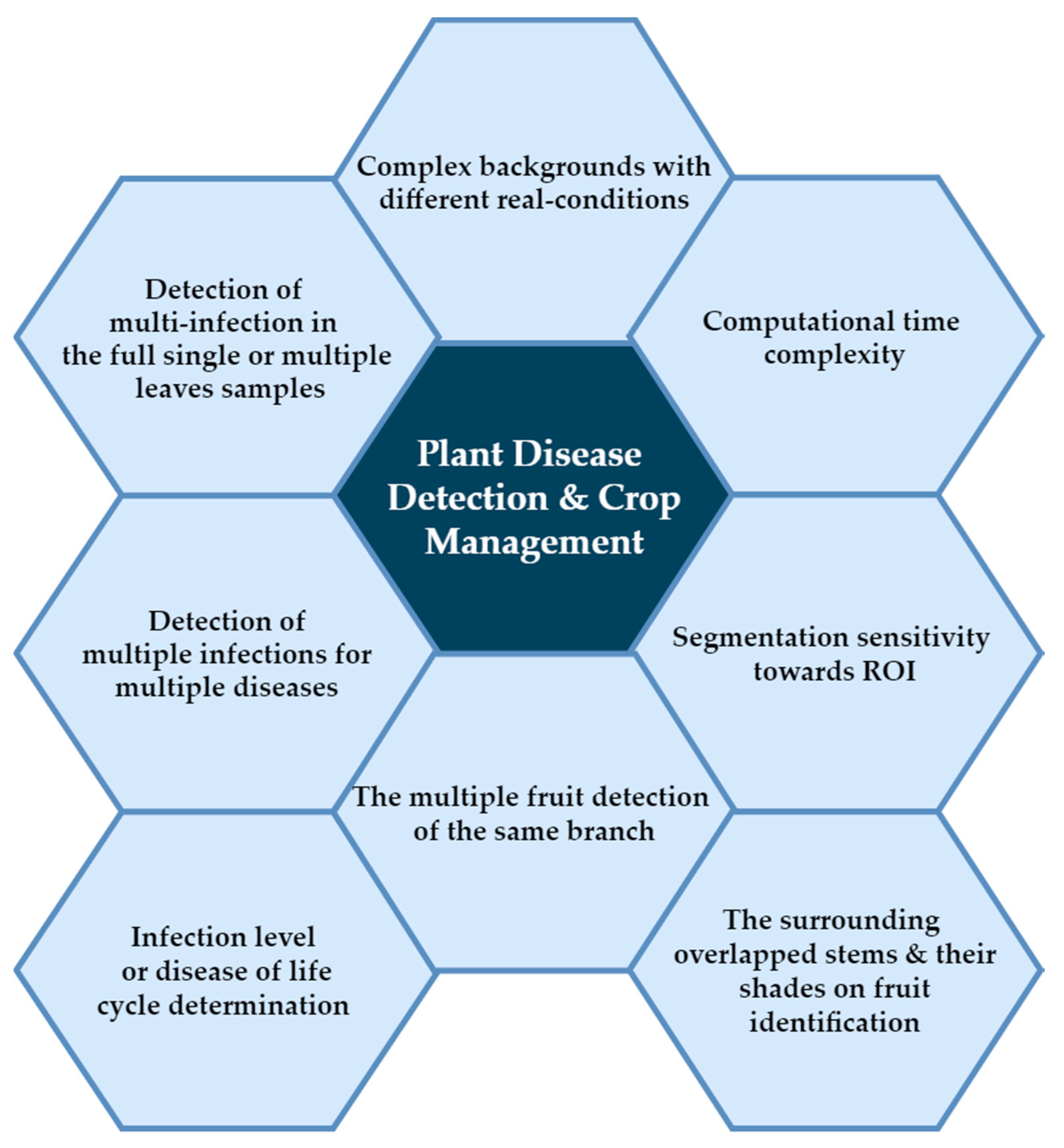
2. Deep Learning Challenges
3. Feature Representation in Shallow Classifiers
3.1. Analysis Measures
3.2. Segmentation
4. Evaluation Measures
- Specificity: is the ratio of the true-negative samples to all healthy samples (true-negative and false-positive). This measure is used to evaluate the performance of a proposed model in predicting true-negative cases.
- Accuracy: is the ratio of the correctly classified samples to the total number of classified samples. this measure is used to evaluate the overall performance of a proposed model.
- Precision/positive predictive value (PPV): is the ratio of the correctly classified samples as infected to all the identified samples as infected (TP+FP).
- F1 Score: is the consistency mean of sensitivity and precision, in the case where the imbalance of false positive/negative samples is important to be measured.
- Coefficient of Quartile Deviation: measures the variability of among the image samples themselves and around the average. low coefficient value means low dispersion. Whereas, Q3 represents the observations that have upper quartile, Q1 represents the observations that have lower quartile [30].
5. Feature Representation in Deep Classifiers
5.1. Training and Transfer Learning
5.2. Feature Visualisation
5.3. Architectures
5.4. Concatenation of Additional Information

| Fruit Detection Architectures and Plant Disease Detection Architectures | ||||
|---|---|---|---|---|
| Study | Objective | No. of Images | Analysis | Evaluation |
| [32] | Cucumber detection | 255 images containing 218 cucumber fruits | Weaknesses: Difficulty of extracting the fruits from image samples with complex backgrounds and overlapping stems of the same colour. Architecture strength: Multi-path CNN suggested the replacement of the SoftMax with SVM classifier for better feature extraction. ROI analysis based on the transformation of the colour space to 15 colours and the PCA analytical tool. Findings: Decreased feature probability for the SVM classifier (the input image). Despite the obstructions with overlapping stems, which are almost the same colour as the fruits, this method was able to recognise both. | 90% correct recognition |
| [107] | Tomato detection | 966 images containing 3465 tomato fruits | Weaknesses: False positive detection in some cases of severe fruit occlusion or overlapping leaves. Architecture strength: YOLO-Tomato utilised a dense architecture inspired by DenseNet. It employed circular boxes rather than rectangular boxes. Findings: The model enabled the re-usage of features at successive layers for better feature extraction, which helped address the gradient vanishing problem by decreasing overlapping and occlusion effects, resulting in improved tomato localisation. | 94.58% correct recognition |
| [108] | Grape detection | 300 images containing 4432 grape clusters | Weaknesses: Counting grapes is very challenging due to the variability in shapes, sizes, compactness and colour. Architecture strength: Mask R-CNN with ResNet 101 as a backbone. Findings: Simultaneous localisation and mapping algorithms allowed the model to overcome these challenges and helped to prevent double counting of fruits. | 0.91 F1-score |
| [109] | Branch fruit recognition | 12,443 images containing apples, nectarines, apricots, peaches, sour cherries, plums | Weaknesses: In cases of apples overlapping with leaves, the activation map was more sensitive towards the leaves than the fruits. Architecture strength: Composed of three convolutional layers, max-pooling and fully connected layer, and used global average pooling rather than traditional flattening techniques. Findings: Very fast compared to ResNet50, making it appropriate for precision horticulture. Suitable for use with small training datasets. | 99.76% accuracy; 0.997 F1-score |
| [110] | Apple and orange detection | 5142 apples in 878 images mix of close-up and distant views | Weaknesses: Without applying any pre-processing, light and shadows of the overlapping leaves impeded the Yolo-v3 architecture’s detection of 90% of the fruits. Architecture strength: Applying pre-processing techniques (contrast increase, slight blurring, thickening of the borders). Findings: Pre-processing increased efficacy. | 90.8% detection rate; 0.92 F1-score |
| [111] | Apple detection | 1200 images 100 contained no fruits | Weaknesses: Detection failures in cases of overlapping fruits. The LedNet model was time-consuming. Architecture strength: ResNet model implemented as a backbone. Both FPN and atrous spatial pyramid pooling employed within the model. Findings: The used techniques achieved better ROI detection on the feature map than the convolutional fixed-size kernel used in one-stage architecture. | 0.849 F1-score |
| [112] | Kiwi detection | 1000 images – mix of RGB and near-infrared (NIR) modalities, containing 39,678 fruits | Weaknesses: No public kiwi fruit datasets available, presenting an obstacle to comparing the study with different datasets. Architecture strength: The VGG16 network was altered to handle RGB and NIR parameters separately but simultaneously, then fine-tuned. Findings: Fast detection and increased accuracy. | 90% accuracy |
| [113] | Orange detection | 200 images | Weaknesses False negatives when distinguishing between fruits and branches. Architecture strength: Mask R-CNN with ResNet-101 as a feature extractor backbone, utilising pixel-wise segmentation. Findings RGB + HVC images enhanced the segmentation phase. | 0.9753 precision |
| [114] | Sugar beet leaf disease detection | 155 beet leaf images, 97 containing mild diseases | Weaknesses: High time consumption associated with gradient descent repetition due to the high-resolution image samples and the large volume of stride and padding used in the convolution layers (applied at the training phase). Architecture strength: Updated Faster R-CNN; adjusted the parameters of the model to be suitable for the number of objects in the dataset. The size of the input image, the number of filters, the strides and the padding size increased in the first two convolutional layers. Findings: Provided detailed information about the diseased corner regions of the leaves. | 95.48% accuracy |
| [115] | Detection of insects in stored grain | 22,043 images containing 108,486 insects | Weaknesses: False negatives for extremely small-sized insect due to unfit anchor scale contributions that considered these insects as ground truth. Architecture strength: MSI-Detector with FPN backbone; an architecture proposed to extract multi-/small-scale insects surrounded by anchors of corresponding sizes. Included pyramid levels to handle features. Findings: Multi-scale insect detection. | 94.77% mAP |
| [116] | Detection of insects on tea plants | 75,222 images of 102 classes (including mites and butterflies) from different datasets | Weaknesses: Spectral residual (SPE) technique highlighted fewer pixels than other techniques. Architecture strength: FusionSUM ensemble network with three different saliency techniques (graph-based visual saliency, cluster-based saliency detection and SPE) applied for feature extraction with different classifiers. Findings: The saliency techniques used improved the performance of all the applied networks; DenseNet and MobileNet were more convenient for large-scale datasets than small-scale ones. | 92.43% recognition accuracy |
| [117] | Banana disease and pest detection (affecting different parts of the plant) | 30,952 images containing 9000 leaf images, 14,376 cut fruits, 1427 fruit bunches, 1406 pseudostems | Weaknesses: Many variations experienced by the loss function, especially in the entire plant and leaf models, which had low accuracy compared to the other models. Architecture strength: Faster R-CNN with InceptionV2 as a backbone was the best choice for training, object localisation and increased feature extraction among several architectures that were applied. Findings: This method achieved high accuracy with overlapping dried leaves of the same plant and the surrounding plants. | 95% accuracy for pseudostems and fruit bunches |
| [118] | Tomato disease and pest detection | 15,000 images (146,912 labelled) | Weaknesses Time-consuming pyramid architecture. Architecture strength: Improved Yolo-V3, a pyramid architecture and multi-scale images training were applied. The fully connected layer was replaced with a convolutional operation to accommodate the lower number of parameters. Findings: This method improved multi-scale object detection and object dimension identification. | 92.39% recognition accuracy |
| [119] | Apple leaf disease detection | 26,377 images categorised into five diseases | Weaknesses: An overfitting problem, perhaps as the wide and deep model selected for better feature extraction had many parameters. Architecture strength: VGG-INCEP; replacement of the first two convolutional layers of VGG16 architecture with others from GoogLeNet Inception for pre-training. SSD-INCEP with Rainbow concatenation employed to fuse features. Findings: This method achieved better feature extraction of different scales and feature fusion. | 97.12% recognition accuracy; 78.80% mAP |
| [120] | Crop disease detection | 54,306 images categorised into 14 crop species with 26 diseases | Weaknesses: Essentially depended on the PlantVillage dataset, where image samples have unified backgrounds. Architecture strength: dCrop; an architecture proposed as a mobile application to detect diseases even without internet access. Findings: Three training architectures. The highest accuracy was achieved using ResNet 50, which was able to learn residuals and presented better predictions. | 99.24% recognition accuracy |
| [121] | Rice sheaf and stem disease and pest detection | 5320 images of three diseases and 4290 frames of five videos | Weaknesses: Lesion detection in videos is considered very challenging. Hence, the model was trained using still pictures, and avoiding blurry or distorted frames where the boundaries of the lesion are not clear. Architecture strength: DCNN Backbone formed of four blocks, with the ReLU layer in a new position to allow for better convergence. Findings: Many architectures have low detection performance for blurry image samples. | 90.0 video spot precision |
| [122] | Maize leaf disease detection | 6267 unmanned aerial vehicle images containing 25,508 lesions | Weaknesses: The large number of sub-images per lesion caused an overfitting problem. Therefore, data were re-split to generate one image per lesion for better training distribution. Architecture strength: Three-stage pipeline model, making full use of the high-resolution image samples. Findings: Adding contextual information in the training phase led to improved putative lesion determination and increased accuracy. | 95.1% precision |
6. Realistic Datasets
7. Data Augmentation
8. Discussion
- Shallow models are recommended for small datasets. These classifiers can achieve 100% accuracy despite the difficulties of choosing the best analytical techniques to analyse lesion spots and the optimal accompaniment classifier.
- To achieve variety in training image samples, datasets can be collected from different resources. These can take into consideration different natural lighting angles (Figure 7) and conditions with complex overlapping surroundings (Figure 8). This includes the standard augmentation techniques (pixel-wise, rotation, resizing and blurring) and the artificially generated images.
- Environmental and geographical information has a significant impact on determining whether the symptoms of affected leaves are caused by the surrounding factors or leaf disease.
- To validate the accurate performance of a classifier, researchers should test its ability to differentiate similar symptoms related to different diseases (e.g., Northern leaf blight and anthracnose leaf blight in maize leaves). To achieve high accuracy, models should be trained with the target disease dataset [122] and images of similar symptoms on different organs (e.g., withered stems and leaves in rice) [121], as well as the typical viral symptoms in leaves of (melon, zucchini, cucurbit, cucumber, papaya watermelon, cucumber) [33].
9. Conclusions and Future Orientations
- Mild symptoms of some plant diseases in their early life cycles.
- Some lesion spots have no determined shapes.
- Plant health considerations via monitoring growth and ripeness life cycle of fruits and leaves.
- Automated labelling and auto segmentation of image samples based GANs.
- The usage of hyperspectral data to feed deep classifiers is a recently developed technique that is recommended for the early detection of plant disease life cycles and the healthy leaf life cycle to differentiate it from a diseased leaf.
- Lastly, future work will include several deep learning models for early classification and detection of plant disease due to huge improvements in deep learning models and the availability in plant datasets. Therefore, that will reflect positively on the quality of plants for future generations.
Author Contributions
Funding
Conflicts of Interest
References
- Esteva, A.; Robicquet, A.; Ramsundar, B.; Kuleshov, V.; Depristo, M.; Chou, K.; Cui, C.; Corrado, G.; Thrun, S.; Dean, J. A guide to deep learning in healthcare. Nat. Med. 2019, 25, 24–29. [Google Scholar] [CrossRef] [PubMed]
- Yu, J.; Mei, X.; Porikli, F.; Corso, J. Machine learning for big visual analysis. Mach. Vis. Appl. 2018, 29, 929–931. [Google Scholar] [CrossRef] [Green Version]
- Tan, Q.; Liu, N.; Hu, X. Deep Representation Learning for Social Network Analysis. Front. Big Data 2019, 2, 2. [Google Scholar] [CrossRef] [Green Version]
- Purwins, H.; Li, B.; Virtanen, T.; Schlüter, J.; Chang, S.-Y.; Sainath, T.N. Deep Learning for Audio Signal Processing. IEEE J. Sel. Top. Signal Process. 2019, 13, 206–219. [Google Scholar] [CrossRef] [Green Version]
- Mnih, V.; Kavukcuoglu, K.; Silver, D.; Graves, A.; Antonoglou, I.; Wierstra, D.; Riedmiller, M. Playing atari with deep reinforcement learning. arXiv 2013, arXiv:1312.5602. [Google Scholar]
- Wang, Y. A new concept using LSTM Neural Networks for dynamic system identification. In Proceedings of the 2017 American Control Conference (ACC), Seattle, WA, USA, 24–26 May 2017; pp. 5324–5329. [Google Scholar]
- Debnath, T.; Biswas, T.; Ashik, M.H.; Dash, S. Auto-Encoder Based Nonlinear Dimensionality Reduction of ECG data and Classification of Cardiac Arrhythmia Groups Using Deep Neural Network. In Proceedings of the 2018 4th International Conference on Electrical Engineering and Information & Communication Technology (iCEEiCT), Dhaka, Bangladesh, 13–15 September 2018; pp. 27–31. [Google Scholar]
- Alom, Z.; Taha, T.M.; Yakopcic, C.; Westberg, S.; Sagan, V.; Nasrin, M.S.; Hasan, M.; Van Essen, B.C.; Awwal, A.A.S.; Asari, V.K. A State-of-the-Art Survey on Deep Learning Theory and Architectures. Electronics 2019, 8, 292. [Google Scholar] [CrossRef] [Green Version]
- Krizhevsky, A.; Sutskever, I.; Hinton, G.E. ImageNet Classification with Deep Convolutional Neural Networks. In Proceedings of the Advances in Neural Information Processing Systems (NIPS), Lake Tahoe, NV, USA, 3–6 December 2012; pp. 1097–1105. [Google Scholar]
- Litjens, G.; Kooi, T.; Bejnordi, B.E.; Setio, A.A.A.; Ciompi, F.; Ghafoorian, M.; Van Der Laak, J.A.; Van Ginneken, B.; Sánchez, C.I. A survey on deep learning in medical image analysis. Med. Image Anal. 2017, 42, 60–88. [Google Scholar] [CrossRef] [Green Version]
- Alzubaidi, L.; Fadhel, M.A.; Al-Shamma, O.; Zhang, J.; Duan, Y. Deep Learning Models for Classification of Red Blood Cells in Microscopy Images to Aid in Sickle Cell Anemia Diagnosis. Electronics 2020, 9, 427. [Google Scholar] [CrossRef] [Green Version]
- Kamilaris, A.; Prenafeta-Boldú, F.X. Deep learning in agriculture: A survey. Comput. Electron. Agric. 2018, 147, 70–90. [Google Scholar] [CrossRef] [Green Version]
- Güzel, M. The Importance of Good Agricultural Practices (GAP) in the Context of Quality Practices in Agriculture and a Sample Application. Ph.D. Thesis, Dokuz Eylül University, İzmir, Turkey, 2012. [Google Scholar]
- Liakos, K.G.; Busato, P.; Moshou, D.; Pearson, S.; Bochtis, D. Machine Learning in Agriculture: A Review. Sensors 2018, 18, 2674. [Google Scholar] [CrossRef] [PubMed] [Green Version]
- Savary, S.; Ficke, A.; Aubertot, J.-N.; Hollier, C. Crop losses due to diseases and their implications for global food production losses and food security. Food Secur. 2012, 4, 519–537. [Google Scholar] [CrossRef]
- Lamichhane, J.R.; Venturi, V. Synergisms between microbial pathogens in plant disease complexes: A growing trend. Front. Plant Sci. 2015, 6, 385. [Google Scholar] [CrossRef] [Green Version]
- Pandey, P.; Irulappan, V.; Bagavathiannan, M.V.; Senthil-Kumar, M. Impact of Combined Abiotic and Biotic Stresses on Plant Growth and Avenues for Crop Improvement by Exploiting Physio-morphological Traits. Front. Plant Sci. 2017, 8, 537. [Google Scholar] [CrossRef] [PubMed] [Green Version]
- Hari, D.P.R.K. Review on Fast Identification and Classification in Cultivation. Int. J. Adv. Sci. Technol. 2020, 29, 3498–3512. [Google Scholar]
- Barbedo, J.G.A. Factors influencing the use of deep learning for plant disease recognition. Biosyst. Eng. 2018, 172, 84–91. [Google Scholar] [CrossRef]
- Arsenovic, M.; Karanovic, M.; Sladojevic, S.; Anderla, A.; Stefanovic, D. Solving Current Limitations of Deep Learning Based Approaches for Plant Disease Detection. Symmetry 2019, 11, 939. [Google Scholar] [CrossRef] [Green Version]
- Tian, K.; Li, J.; Zeng, J.; Evans, A.; Zhang, L. Segmentation of tomato leaf images based on adaptive clustering number of K-means algorithm. Comput. Electron. Agric. 2019, 165, 104962. [Google Scholar] [CrossRef]
- Amara, J.; Bouaziz, B.; Algergawy, A. A Deep Learning-Based Approach for Banana Leaf Diseases Classification. In Lecture Notes in Informatics (LNI); Gesellschaft für Informatik: Bonn, Germany, 2017; Volume 266, pp. 79–88. [Google Scholar]
- Zhang, S.; Huang, W.; Zhang, C. Three-channel convolutional neural networks for vegetable leaf disease recognition. Cogn. Syst. Res. 2019, 53, 31–41. [Google Scholar] [CrossRef]
- Ngugi, L.C.; Abdelwahab, M.M.; Abo-Zahhad, M. Recent advances in image processing techniques for automated leaf pest and disease recognition—A review. Inf. Process. Agric. 2020. [Google Scholar] [CrossRef]
- Sharif, M.; Khan, M.A.; Iqbal, Z.; Azam, M.F.; Lali, M.I.U.; Javed, M.Y. Detection and classification of citrus diseases in agriculture based on optimized weighted segmentation and feature selection. Comput. Electron. Agric. 2018, 150, 220–234. [Google Scholar] [CrossRef]
- Anjna; Sood, M.; Singh, P.K. Hybrid System for Detection and Classification of Plant Disease Using Qualitative Texture Features Analysis. Procedia Comput. Sci. 2020, 167, 1056–1065. [Google Scholar]
- Baranwal, S.; Khandelwal, S.; Arora, A. Deep Learning Convolutional Neural Network for Apple Leaves Disease Detection. In Proceedings of the International Conference on Sustainable Computing in Science, Technology & Management (SUSCOM-2019), Jaipur, India, 26–28 February 2019; pp. 260–267. [Google Scholar]
- Kc, K.; Yin, Z.; Wu, M.; Wu, Z. Depthwise separable convolution architectures for plant disease classification. Comput. Electron. Agric. 2019, 165, 104948. [Google Scholar] [CrossRef]
- Chouhan, S.S.; Singh, U.P.; Kaul, A.; Jain, S. A data repository of leaf images: Practice towards plant conservation with plant pathology. In Proceedings of the 4th International Conference on Information Systems and Computer Networks (ISCON), Mathura, India, 21–22 November 2019; IEEE: Piscataway, NJ, USA, 2019; pp. 700–707. [Google Scholar]
- Sharma, P.; Berwal, Y.P.S.; Ghai, W. Performance analysis of deep learning CNN models for disease detection in plants using image segmentation. Inf. Process. Agric. 2019, in press. [Google Scholar] [CrossRef]
- Wang, F.; Wang, R.; Xie, C.; Yang, P.; Liu, L. Fusing multi-scale context-aware information representation for automatic in-field pest detection and recognition. Comput. Electron. Agric. 2020, 169, 105222. [Google Scholar] [CrossRef]
- Mao, S.; Li, Y.; Ma, Y.; Zhang, B.; Zhou, J.; Wang, K. Automatic cucumber recognition algorithm for harvesting robots in the natural environment using deep learning and multi-feature fusion. Comput. Electron. Agric. 2020, 170, 105254. [Google Scholar] [CrossRef]
- Fujita, E.E.; Uga, H.; Kagiwada, S.; Iyatomi, H. A Practical Plant Diagnosis System for Field Leaf Images and Feature Visualization. Int. J. Eng. Technol. 2018, 7, 49–54. [Google Scholar] [CrossRef] [Green Version]
- Bresilla, K.; Perulli, G.D.; Boini, A.; Morandi, B.; Grappadelli, L.C.; Manfrini, L. Single-Shot Convolution Neural Networks for Real-Time Fruit Detection Within the Tree. Front. Plant Sci. 2019, 10, 611. [Google Scholar] [CrossRef] [Green Version]
- Boulent, J.; Foucher, S.; Théau, J.; St-Charles, P.-L. Convolutional Neural Networks for the Automatic Identification of Plant Diseases. Front. Plant Sci. 2019, 10, 941. [Google Scholar] [CrossRef] [Green Version]
- Liu, L.; Ouyang, W.; Wang, X.; Fieguth, P.; Chen, J.; Liu, X.; Pietikäinen, M. Deep learning for generic object detection: A survey. Int. J. Comput. Vis. 2020, 128, 261–318. [Google Scholar] [CrossRef] [Green Version]
- Alzubaidi, L.; Fadhel, M.A.; Oleiwi, S.R.; Al-Shamma, O.; Zhang, J. DFU_QUTNet: Diabetic foot ulcer classification using novel deep convolutional neural network. Multimed. Tools Appl. 2020, 79, 15655–15677. [Google Scholar] [CrossRef]
- Khan, A.; Sohail, A.; Zahoora, U.; Qureshi, A.S. A survey of the recent architectures of deep convolutional neural networks. Artif. Intell. Rev. 2020, 1–62. [Google Scholar] [CrossRef] [Green Version]
- Li, Y.; Huang, C.; Ding, L.; Li, Z.; Pan, Y.; Gao, X. Deep learning in bioinformatics: Introduction, application, and perspective in the big data era. Methods 2019, 166, 4–21. [Google Scholar] [CrossRef] [PubMed] [Green Version]
- Gregor, K.; LeCun, Y. Learning fast approximations of sparse coding. In Proceedings of the 27th International Conference on Machine Learning, Omnipress, WI, USA, 24–27 June 2010; pp. 399–406. [Google Scholar]
- Ranzato, M.; Mnih, V.; Susskind, J.M.; Hinton, G.E. Modeling natural images using gated MRFs. IEEE Trans Pattern Anal Mach Intell. 2013, 35, 2206–2222. [Google Scholar] [CrossRef] [PubMed] [Green Version]
- Krause, J.; Sapp, B.; Howard, A.; Zhou, H.; Toshev, A.; Duerig, T.; Fei-Fei, L. The unreasonable effectiveness of noisy data for fine-grained recognition. In Proceedings of the 14th European Conference on Computer Vision, Proceedings Part III, Amsterdam, The Netherlands, 11–14 October 2016; Springer: Berline/Heidelberg, Germany, 2016; pp. 301–320. [Google Scholar]
- Torralba, A.; Fergus, B.; Freeman, W.T. 80 million tiny images: A large data set for nonparametric object and scene recognition. IEEE Trans. Pattern Anal. Mach. Intell. 2008, 30, 1958–1970. [Google Scholar] [CrossRef] [PubMed]
- Lu, J.; Young, S.; Arel, I.; Holleman, J. A 1 TOPS/W Analog Deep Machine-Learning Engine With Floating-Gate Storage in 0.13 µm CMOS. IEEE J. Solid-State Circuits 2015, 50, 270–281. [Google Scholar] [CrossRef]
- Micheli, A. Neural network for graphs: A contextual constructive approach. IEEE Trans. Neural Netw. 2009, 20, 498–511. [Google Scholar] [CrossRef]
- Hinton, G.; Deng, L.; Yu, D.; Dahl, G.; Mohamed, A.-A.; Jaitly, N.; Senior, A.; Vanhoucke, V.; Nguyen, P.; Sainath, T.; et al. Deep neural networks for acoustic modeling in speech recognition: The shared views of four research groups. IEEE Signal Process. Mag. 2012, 29, 82–97. [Google Scholar] [CrossRef]
- Dahl, G.E.; Yu, D.; Deng, L.; Acero, A. Context-dependent pre-trained deep neural networks for large-vocabulary speech recognition. IEEE Trans. Audio Speech Lang. Process. 2012, 20, 30–42. [Google Scholar] [CrossRef] [Green Version]
- Hong, S.; Kim, H. An integrated GPU power and performance model. In Proceedings of the 37th Annual International Symposium on Computer architecture, Saint-Malo, France, 19–23 June 2010; ACM: New York, NY, USA, 2010; Volume 38, pp. 280–289. [Google Scholar]
- Fadhel, M.A.; Al-Shamma, O.; Oleiwi, S.R.; Taher, B.H.; Alzubaidi, L. Real-time PCG diagnosis using FPGA. In Proceedings of the International Conference on Intelligent Systems Design and Applications, Vellore, India, 6–8 December 2018; Springer: Berlin/Heidelberg, Germany, 2018; Volume 1, pp. 518–529. [Google Scholar]
- Al-Shamma, O.; Fadhel, M.A.; Hameed, R.A.; Alzubaidi, L.; Zhang, J. Boosting convolutional neural networks performance based on FPGA accelerator. In Proceedings of the International Conference on Intelligent Systems Design and Applications (ISDA 2018), Vellore, India, 6–8 December 2018; Springer: Cham, Switzerland, 2018; Volume 1, pp. 509–517. [Google Scholar]
- Wang, C.; Gong, L.; Yu, Q.; Li, X.; Xie, Y.; Zhou, X. DLAU: A scalable deep learning accelerator unit on FPGA. IEEE Trans. Comput.-Aided Des. Integr. Circuits Syst. 2016, 36, 513–517. [Google Scholar]
- Zhang, C.; Li, P.; Sun, G.; Guan, Y.; Xiao, B.; Cong, J. Optimizing FPGA-based accelerator design for deep convolutional neural networks. In Proceedings of the ACM/SIGDA International Symposium on Field-Programmable Gate Arrays, Monterey, CA, USA, 22–24 February 2015; ACM: New York, NY, USA, 2015; pp. 161–170. [Google Scholar]
- Islam, M.; Dinh, A.; Wahid, K.; Bhowmik, P. Detection of potato diseases using image segmentation and multiclass support vector machine. In Proceedings of the 2017 IEEE 30th Canadian Conference on Electrical and Computer Engineering (CCECE), Windsor, ON, Canada, 30 April–3 May 2017; pp. 1–4. [Google Scholar] [CrossRef] [Green Version]
- Deepa, S.; Umarani, R. Steganalysis on Images using SVM with Selected Hybrid Features of Gini Index Feature Selection Algorithm. Int. J. Adv. Res. Comput. Sci. 2017, 8, 1503–1509. [Google Scholar]
- Sannakki, S.S.; Rajpurohit, V.S.; Nargund, V.B. SVM-DSD: SVM Based Diagnostic System for the Detection of Pomegranate Leaf Diseases. In Proceedings of the International Conference on Advances in Computing. Advances in Intelligent Systems and Computing, Kochi, Kerala, India, 29–31 August 2013; Kumar, M.A.R.S., Kumar, T., Eds.; Springer: New Delhi, India, 2013; Volume 174. [Google Scholar]
- Sandika, B.; Avil, S.; Sanat, S.; Srinivasu, P. Random Forest Based Classification of Diseases in Grapes from Images Captured in Uncontrolled Environments. In Proceedings of the 2016 IEEE 13th International Conference on Signal Processing (ICSP), Chengdu, China, 6–10 November 2016; pp. 1775–1780. [Google Scholar]
- Guettari, N.; Capelle-Laize, A.S.; Carre, P. Blind image steganalysis based on evidential K-Nearest Neighbors. In Proceedings of the 2016 IEEE International Conference on Image Processing (ICIP), Phoenix, AZ, USA, 25–28 September 2016; pp. 2742–2746. [Google Scholar]
- Hossain, E.; Hossain, F.; Rahaman, M.A. A Color and Texture Based Approach for the Detection and Classification of Plant Leaf Disease Using KNN Classifier. In Proceedings of the 2019 International Conference on Electrical, Computer and Communication Engineering (ECCE), Cox’s Bazar, Bangladesh, 7–9 February 2019; pp. 1–6. [Google Scholar]
- Haralick, R.M.; Shanmugam, K. Textural features for image classification. IEEE Trans. Syst. Man. Cybern. 1973, 6, 610–621. [Google Scholar] [CrossRef] [Green Version]
- Albregtsen, F. Statistical Texture Measures Computed from Gray Level Coocurrence Matrices. Image Processing Laboratory, Department of Informatics, University of Oslo Web Site. 1995. Available online: http://www.uio.no/studier/emner/matnat/ifi/INF4300/h08/undervisningsmateriale/glcm.pdf (accessed on 5 November 2008).
- Pei, S.-C.; Cheng, C.-M. Color image processing by using binary quaternion-moment-preserving thresholding technique. IEEE Trans. Image Process. 1999, 8, 614–628. [Google Scholar] [CrossRef]
- Kim, J.; Han, D.; Tai, Y.-W.; Kim, J. Salient Region Detection via High-Dimensional Color Transform and Local Spatial Support. IEEE Trans. Image Process. 2015, 25, 9–23. [Google Scholar] [CrossRef]
- Inamdar, N.; Diggikar, A. Image Processing Based Automatic Leaf Disease Detection System Using K-Means Clustering And SVM. Int. J. Eng. Appl. Manag. Sci. Paradig. (IJEAM) 2019, 54. [Google Scholar]
- Hendrawan, Y.; Fauzi, M.R.; Khoirunnisa, N.S.; Andreane, M.P.O.H.; Umam, C. Development of Colour Co-occurrence Matrix (CCM) Texture Analysis for Biosensing. In IOP Conference Series: Earth and Environmental Science; IOP Publishing Ltd.: Bristol, UK, 2019. [Google Scholar]
- Arivazhagan, S.; Shebiah, R.N.; Ananthi, S.; Varthini, S.V. Detection of unhealthy region of plant leaves and classification of plant leaf diseases using texture features. Agric. Eng. Int. CIGR J. 2013, 15, 211–217. [Google Scholar]
- Qin, J.; Burks, T.F.; Kim, D.G.; Bulanon, D.M. Classification of Citrus Peel Diseases Using Color Texture Feature Analysis. In Proceedings of the Food Processing Automation Conference, Providence, RI, USA, 28–29 June 2008; American Society of Agricultural and Biological Engineers (ASABE): Saint Joseph, MI, USA, 2008. [Google Scholar]
- Singh, V.; Varsha; Misra, A.K. Detection of unhealthy region of plant leaves using image processing and genetic algorithm. In Proceedings of the 2015 International Conference on Advances in Computer Engineering and Applications, Ghaziabad, India, 19–20 March 2015; pp. 1028–1032. [Google Scholar]
- Malik, Z.; Ziauddin, S.; Shahid, A.R.; Safi, A. Detection and Counting of On-Tree Citrus Fruit for Crop Yield Estimation. Int. J. Adv. Comput. Sci. Appl. 2016, 7, 7. [Google Scholar] [CrossRef]
- Sun, Q.-S.; Zeng, S.-G.; Liu, Y.; Heng, P.; Xia, D.-S. A new method of feature fusion and its application in image recognition. Pattern Recognit. 2005, 38, 2437–2448. [Google Scholar] [CrossRef]
- Haghighat, M.B.A.; Abdel-Mottaleb, M.; Alhalabi, W. Discriminant correlation analysis for feature level fusion with application to multimodal biometrics. In Proceedings of the 2016 IEEE International Conference on Acoustics, Speech and Signal Processing (ICASSP), Shanghai, China, 20–25 March 2016; pp. 1866–1870. [Google Scholar]
- Navarro, C.F.; Perez, C.A. Color–Texture Pattern Classification Using Global–Local Feature Extraction, an SVM Classifier, with Bagging Ensemble Post-Processing. Appl. Sci. 2019, 9, 3130. [Google Scholar] [CrossRef] [Green Version]
- Soviany, S.; Sandulescu, V.; Puscoci, S.; Soviany, C. A Biometric System with Hierarchical Feature-level Fusion. In Proceedings of the 2018 10th International Conference on Electronics, Computers and Artificial Intelligence (ECAI), Iasi, Romania, 28–30 June 2018; pp. 1–6. [Google Scholar] [CrossRef]
- Adeel, A.; Khan, M.A.; Sharif, M.; Azam, F.; Shah, J.H.; Umer, T.; Wan, S. Diagnosis and recognition of grape leaf diseases: An automated system based on a novel saliency approach and canonical correlation analysis based multiple features fusion. Sustain. Comput. Inform. Syst. 2019, 24, 100349. [Google Scholar] [CrossRef]
- Vetal, S.; Khule, R.S. Tomato Plant Disease Detection using Image Processing. Int. J. Adv. Res. Comput. Commun. Eng. 2017, 6, 293–297. [Google Scholar] [CrossRef]
- Shin, J.; Chang, Y.K.; Heung, B.; Nguyen-Quang, T.; Price, G.W.; Al-Mallahi, A. Effect of directional augmentation using supervised machine learning technologies: A case study of strawberry powdery mildew detection. Biosyst. Eng. 2020, 194, 49–60. [Google Scholar] [CrossRef]
- Elsalamony, H.A. Healthy and unhealthy red blood cell detection in human blood smears using neural networks. Micron 2016, 83, 32–41. [Google Scholar] [CrossRef]
- Das, P.K.; Meher, S.; Panda, R.; Abraham, A. A Review of Automated Methods for the Detection of Sickle Cell Disease. IEEE Rev. Biomed. Eng. 2020, 13, 309–324. [Google Scholar] [CrossRef] [PubMed]
- Shin, H.-C.; Roth, H.R.; Gao, M.; Lu, L.; Xu, Z.; Nogues, I.; Yao, J.; Mollura, D.; Summers, R.M.; Hoo-Chang, S. Deep Convolutional Neural Networks for Computer-Aided Detection: CNN Architectures, Dataset Characteristics and Transfer Learning. IEEE Trans. Med Imaging 2016, 35, 1285–1298. [Google Scholar] [CrossRef] [PubMed] [Green Version]
- Brahimi, M.; Arsenovic, M.; Laraba, S.; Sladojevic, S.; Boukhalfa, K.; Moussaoui, A. Deep Learning for Plant Diseases: Detection and Saliency Map Visualisation. In Primitive Interaction Design; Springer Science and Business Media LLC: Cham, Switzerland, 2018; pp. 93–117. [Google Scholar]
- Kessentini, Y.; Besbes, M.D.; Ammar, S.; Chabbouh, A. A two-stage deep neural network for multi-norm license plate detection and recognition. Expert Syst. Appl. 2019, 136, 159–170. [Google Scholar] [CrossRef]
- Chen, J.; Chen, J.; Zhang, D.; Sun, Y.; Nanehkaran, Y. Using deep transfer learning for image-based plant disease identification. Comput. Electron. Agric. 2020, 173, 105393. [Google Scholar] [CrossRef]
- Turkoglu, M.; Hanbay, D. Leaf-based plant species recognition based on improved local binary pattern and extreme learning machine. Phys. A Stat. Mech. Its Appl. 2019, 527, 121297. [Google Scholar] [CrossRef]
- Raghu, M.; Zhang, C.; Kleinberg, J.; Bengio, S. Transfusion: Understanding transfer learning for medical imaging. Adv. Neural Inf. Prcoess. Syst. 2019, 3347–3357. [Google Scholar]
- Alzubaidi, L.; Al-Shamma, O.; Fadhel, M.A.; Farhan, L.; Zhang, J.; Duan, Y. Optimizing the Performance of Breast Cancer Classification by Employing the Same Domain Transfer Learning from Hybrid Deep Convolutional Neural Network Model. Electronics 2020, 9, 445. [Google Scholar] [CrossRef] [Green Version]
- Alzubaidi, L.; Fadhel, M.A.; Al-Shamma, O.; Zhang, J.; Santamaría, J.; Duan, Y.; Oleiwi, S.R. Towards a Better Understanding of Transfer Learning for Medical Imaging: A Case Study. Appl. Sci. 2020, 10, 4523. [Google Scholar] [CrossRef]
- Razavian, A.S.; Azizpour, H.; Sullivan, J.; Carlsson, S. CNN Features Off-the-Shelf: An Astounding Baseline for Recognition. In Proceedings of the 2014 IEEE Conference on Computer Vision and Pattern Recognition Workshops, Columbus, OH, USA, 24–27 July 2014; pp. 512–519. [Google Scholar]
- Lee, S.H.; Goëau, H.; Bonnet, P.; Joly, A. New perspectives on plant disease characterization based on deep learning. Comput. Electron. Agric. 2020, 170, 105220. [Google Scholar] [CrossRef]
- Atabay, H.A. Deep residual learning for tomato plant leaf disease identification. J. Theor. Appl. Inf. Technol. 2017, 95, 6800–6808. [Google Scholar]
- Selvaraju, R.R.; Cogswell, M.; Das, A.; Vedantam, R.; Parikh, D.; Batra, D. Grad-CAM: Visual Explanations from Deep Networks via Gradient-Based Localization. In Proceedings of the 2017 IEEE International Conference on Computer Vision (ICCV), Venice, Italy, 22–29 October 2017; pp. 618–626. [Google Scholar]
- Menikdiwela, M.; Nguyen, C.V.; Li, H.; Shaw, M. CNN-based small object detection and visualization with feature activation mapping. In Proceedings of the 2017 International Conference on Image and Vision Computing New Zealand (IVCNZ), Christchurch, New Zealand, 4–6 December 2017; pp. 1–5. [Google Scholar] [CrossRef]
- Brahimi, M.; Mahmoudi, S.; Boukhalfa, K.; Moussaoui, A. Deep interpretable architecture for plant diseases classification. arXiv 2019, arXiv:1905.13523. [Google Scholar]
- Saleem, M.H.; Potgieter, J.; Arif, K. Plant Disease Detection and Classification by Deep Learning. Plants 2019, 8, 468. [Google Scholar] [CrossRef] [PubMed] [Green Version]
- Toda, Y.; Okura, F. How Convolutional Neural Networks Diagnose Plant Disease. Plant Phenomics 2019, 2019, 9237136. [Google Scholar] [CrossRef]
- Jung, D.; Jung, W.; Kim, A.B.; Lee, S.; Rhee, W.; Ahn, J.H. Restructuring Batch Normalization to Accelerate CNN Training. arXiv 2018, arXiv:1807.01702. [Google Scholar]
- Karthik, R.; Hariharan, M.; Anand, S.; Mathikshara, P.; Johnson, A.; Menaka, R. Attention embedded residual CNN for disease detection in tomato leaves. Appl. Soft Comput. 2020, 86, 105933. [Google Scholar]
- Huang, G.; Liu, Z.; Van Der Maaten, L.; Weinberger, K.Q. Densely Connected Convolutional Networks. In Proceedings of the 2017 IEEE Conference on Computer Vision and Pattern Recognition (CVPR), Honolulu, HI, USA, 21–26 July 2017; pp. 2261–2269. [Google Scholar]
- He, K.; Zhang, X.; Ren, S.; Sun, J. Deep Residual Learning for Image Recognition. In Proceedings of the IEEE Conference on Computer Vision and Pattern Recognition (CVPR), Las Vegas, NV, USA, 26 June–1 July 2016; pp. 770–778. [Google Scholar]
- Simonyan, K.; Zisserman, A. Very deep convolutional networks for large-scale image recognition. arXiv 2014, arXiv:1409.1556. [Google Scholar]
- Jiang, Y.; Li, C. Convolutional Neural Networks for Image-Based High-Throughput Plant Phenotyping: A Review. Plant Phenomics 2020, 2020, 4152816. [Google Scholar] [CrossRef] [Green Version]
- Ren, S.; He, K.; Girshick, R.; Sun, J. Faster r-cnn: Towards real-time object detection with region proposal networks. IEEE Trans. Pattern Anal. Mach. Intell. 2017, 39, 1137–1149. [Google Scholar] [CrossRef] [Green Version]
- Jiao, L.; Zhang, F.; Liu, F.; Yang, S.; Li, L.; Feng, Z.; Qu, R. A Survey of Deep Learning-Based Object Detection. IEEE Access 2019, 7, 128837–128868. [Google Scholar] [CrossRef]
- He, K.; Gkioxari, G.; Dollr, P.; Girshick, R. Mask R-cnn. In Proceedings of the 2017 IEEE International Conference on Computer Vision (ICCV), Venice, Italy, 22–29 October 2017; pp. 2980–2988. [Google Scholar]
- Redmon, J.; Farhadi, A. YOLOv3: An Incremental Improvement. arXiv 2018, arXiv:1804.02767. [Google Scholar]
- Lin, T.; Goyal, P.; Girshick, R.; He, K.; Dollr, P. Focal Loss for Dense Object Detection. In Proceedings of the 2017 IEEE International Conference on Computer Vision (ICCV), Venice, Italy, 22–29 October 2017; pp. 2999–3007. [Google Scholar]
- Cruz, A.C.; Luvisi, A.; De Bellis, L.; Ampatzidis, Y. X-FIDO: An Effective Application for Detecting Olive Quick Decline Syndrome with Deep Learning and Data Fusion. Front. Plant Sci. 2017, 8, 1741. [Google Scholar] [CrossRef] [PubMed]
- Zhao, Y.; Liu, L.; Xie, C.; Wang, R.; Wang, F.; Bu, Y.; Zhang, S. An effective automatic system deployed in agricultural Internet of Things using Multi-Context Fusion Network towards crop disease recognition in the wild. Appl. Soft Comput. J. 2020, 86, 106128. [Google Scholar] [CrossRef]
- Liu, G.; Nouaze, J.C.; Touko Mbouembe, P.L.; Kim, J.H. YOLO-Tomato: A Robust Algorithm for Tomato Detection Based on YOLOv3. Sensors 2020, 20, 2145. [Google Scholar] [CrossRef] [PubMed] [Green Version]
- Santos, T.T.; de Souza, L.L.; dos Santos, A.A.; Avila, S. Grape detection, segmentation, and tracking using deep neural networks and three-dimensional association. Comput. Electron. Agric. 2020, 170, 105247. [Google Scholar] [CrossRef] [Green Version]
- Saedi, S.I.; Khosravi, H. A deep neural network approach towards real-time on-branch fruit recognition for precision horticulture. Exp. Syst. Appl. 2020, 159, 113594. [Google Scholar] [CrossRef]
- Kuznetsova, A.; Maleva, T.; Soloviev, V. Using YOLOv3 Algorithm with Pre- and Post-Processing for Apple Detection in Fruit-Harvesting Robot. Agronomy 2020, 10, 1016. [Google Scholar] [CrossRef]
- Kang, H.; Chen, C. Fast implementation of real-time fruit detection in apple orchards using deep learning. Comput. Electron. Agric. 2020, 168, 105108. [Google Scholar] [CrossRef]
- Liu, Z.; Wu, J.; Fu, L.; Majeed, Y.; Feng, Y.; Li, R.; Cui, Y. Improved kiwifruit detection using pre-trained VGG16 with RGB and NIR information fusion. IEEE Access 2020, 8, 2327–2336. [Google Scholar] [CrossRef]
- Ganesh, P.; Volle, K.; Burks, T.F.; Mehta, S.S. Deep orange: Mask R-CNN based orange detection and segmentation. IFAC Pap. 2019, 52, 70–75. [Google Scholar] [CrossRef]
- Ozguven, M.M.; Adem, K. Automatic detection and classification of leaf spot disease in sugar beet using deep learning algorithms. Phys. A Stat. Mech. Appl. 2019, 535, 122537. [Google Scholar] [CrossRef]
- Li, J.; Zhou, H.; Wang, Z.; Jia, Q. Multi-scale detection of stored-grain insects for intelligent monitoring. Comput. Electron. Agric. 2019, 168, 105114. [Google Scholar] [CrossRef]
- Nanni, L.; Maguolo, G.; Pancino, F. Insect pest image detection and recognition based on bio-inspired methods. Ecol. Inf. 2020, 57, 101089. [Google Scholar] [CrossRef] [Green Version]
- Selvaraj, M.G.; Vergara, A.; Ruiz, H.; Safari, N.; Elayabalan, S.; Ocimati, W.; Blomme, G. AI-powered banana diseases and pest detection. Plant Methods 2019, 15, 92. [Google Scholar] [CrossRef]
- Liu, J.; Wang, X. Tomato Diseases and Pests Detection Based on Improved Yolo V3 Convolutional Neural Network. Front. Plant Sci. 2020, 11, 898. [Google Scholar] [CrossRef]
- Jiang, P.; Chen, Y.; Liu, B.; He, D.; Liang, C. Real-Time Detection of Apple Leaf Diseases Using Deep Learning Approach Based on Improved Convolutional Neural Networks. IEEE Access 2019, 7, 59069–59080. [Google Scholar] [CrossRef]
- Pallagani, V.; Khandelwal, V.; Chandra, B.; Udutalapally, V.; Das, D.; Mohanty, S.P. dCrop: A Deep-Learning Based Framework for Accurate Prediction of Diseases of Crops in Smart Agriculture. In Proceedings of the 2019 IEEE International Symposium on Smart Electronic Systems (iSES) (Formerly iNiS) 2019, Rourkela, India, 16–18 December 2019. [Google Scholar] [CrossRef]
- Li, D.; Wang, R.; Xie, C.; Liu, L.; Zhang, J.; Li, R.; Wang, F.; Zhou, M.; Liu, W. A Recognition Method for Rice Plant Diseases and Pests Video Detection Based on Deep Convolutional Neural Network. Sensors 2020, 20, 578. [Google Scholar] [CrossRef] [Green Version]
- Wu, H.; Wiesner-Hanks, T.; Stewart, E.L.; DeChant, C.; Kaczmar, N.; Gore, M.A.; Lipson, H. Autonomous detection of plant disease symptoms directly from aerial imagery. Plant Phenome J. 2019, 2, 1–9. [Google Scholar] [CrossRef]
- Hughes, D.; Salathé, M. An open access repository of images on plant health to enable the development of mobile disease diagnostics. arXiv 2015, arXiv:1511.08060. [Google Scholar]
- Parraga-Alava, J.; Cusme, K.; Loor, A.; Santander, E. Data Article RoCoLe: A robusta coffee leaf images dataset for evaluation of machine learning based methods in plant diseases recognition. Data Brief 2019, 25, 104414. [Google Scholar] [CrossRef]
- Singh, D.; Naman Jain, P.J.; Kayal, P. PlantDoc: A Dataset for Visual Plant Disease Detection. In Proceedings of the 7th ACM IKDD CoDS and 25th COMAD, 2020, Hyderabad, India, 5–7 January 2020. [Google Scholar]
- Rauf, H.T.; Saleem, B.A.; Lali, M.I.U.; Khan, M.A.; Sharif, M.; Bukhari, S.A.C. A citrus fruits and leaves dataset for detection and classification of citrus diseases through machine learning. Data Brief 2019, 26, 104340. [Google Scholar] [CrossRef] [PubMed]
- Zhu, Y.; Aoun, M.; Krijn, M.; Vanschoren, J. Data Augmentation using Conditional Generative Adversarial Networks for Leaf Counting in Arabidopsis Plants. In Proceedings of the 29th British Machine Vision Conference, Newcastle, UK, 3–6 September 2018; pp. 1–11. [Google Scholar]
- Zhu, J.Y.; Park, T.; Isola, P.; Efros, A.A. Unpaired Image-to-Image Translation Using Cycle-Consistent Adversarial Networks. In Proceedings of the IEEE International Conference on Computer Vision, Venice, Italy, 22–29 October 2017; pp. 2223–2232. [Google Scholar]
- Karras, T.; Aila, T.; Laine, S.; Lehtinen, J. Progressive growing of gans for improved quality, stability, and variation. arXiv 2017, arXiv:1710.10196. [Google Scholar]
- Nazki, H.; Yoon, S.; Fuentes, A.; Park, D.S. Unsupervised image translation using adversarial networks for improved plant disease recognition. Comput. Electron. Agric. 2020, 168, 105117. [Google Scholar] [CrossRef]
- Johnson, J.; Alahi, A.; Fei-Fei, L. Perceptual Losses for Real-Time Style Transfer and Super-Resolution. In European Conference on Computer Vision; Springer: Cham, Switzerland, 2016; pp. 694–711. [Google Scholar]
- Cha, M.; Gwon, Y.; Kung, H.T. Adversarial Nets with Perceptual Losses for Text-to-Image Synthesis. In Proceedings of the IEEE 27th International Workshop on Machine Learning for Signal Processing (MLSP), Tokyo, Japan, 25–28 September 2017; pp. 1–6. [Google Scholar]
- Qin, Z.; Liu, Z.; Zhu, P.; Xue, Y. A GAN-based image synthesis method for skin lesion classification. Comput. Methods Progr. Biomed. 2020, 195, 105568. [Google Scholar] [CrossRef] [PubMed]
- Talebi, H.; Milanfar, P. Nima: Neural image assessment. IEEE Trans. Image Process. 2018, 27, 3998–4011. [Google Scholar] [CrossRef] [PubMed] [Green Version]


© 2020 by the authors. Licensee MDPI, Basel, Switzerland. This article is an open access article distributed under the terms and conditions of the Creative Commons Attribution (CC BY) license (http://creativecommons.org/licenses/by/4.0/).
Share and Cite
Hasan, R.I.; Yusuf, S.M.; Alzubaidi, L. Review of the State of the Art of Deep Learning for Plant Diseases: A Broad Analysis and Discussion. Plants 2020, 9, 1302. https://doi.org/10.3390/plants9101302
Hasan RI, Yusuf SM, Alzubaidi L. Review of the State of the Art of Deep Learning for Plant Diseases: A Broad Analysis and Discussion. Plants. 2020; 9(10):1302. https://doi.org/10.3390/plants9101302
Chicago/Turabian StyleHasan, Reem Ibrahim, Suhaila Mohd Yusuf, and Laith Alzubaidi. 2020. "Review of the State of the Art of Deep Learning for Plant Diseases: A Broad Analysis and Discussion" Plants 9, no. 10: 1302. https://doi.org/10.3390/plants9101302