Article

Auto-Machine-Learning Models for Standardized Precipitation Index Prediction in North–Central Mexico

by
Rafael Magallanes-Quintanar
1,*,
Carlos E. Galván-Tejada
1,
Jorge Isaac Galván-Tejada
1,
Hamurabi Gamboa-Rosales
1,
Santiago de Jesús Méndez-Gallegos
2 and
Antonio García-Domínguez
1,*
1
Unidad Académica de Ingeniería Eléctrica, Universidad Autónoma de Zacatecas, Jardín Juárez 147, Centro, Zacatecas 98000, CP, Mexico
2
Colegio de Postgraduados, Campus San Luis Potosí, Salinas de Hidalgo, San Luis Potosí 78622, CP, Mexico
*
Authors to whom correspondence should be addressed.
Climate 2024, 12(7), 102; https://doi.org/10.3390/cli12070102
Submission received: 2 June 2024 / Revised: 2 July 2024 / Accepted: 9 July 2024 / Published: 12 July 2024

Abstract

:
Certain impacts of climate change could potentially be linked to alterations in rainfall patterns, including shifts in rainfall intensity or drought occurrences. Hence, predicting droughts can provide valuable assistance in mitigating the detrimental consequences associated with water scarcity, particularly in agricultural areas or densely populated urban regions. Employing predictive models to calculate drought indices can be a useful method for the effective characterization of drought conditions. This study applied an Auto-Machine-Learning approach to deploy Artificial Neural Network models, aiming to predict the Standardized Precipitation Index in four regions of Zacatecas, Mexico. Climatological time-series data spanning from 1979 to 2020 were utilized as predictive variables. The best models were found using performance metrics that yielded a Mean Squared Error, Mean Absolute Error, and Coefficient of Determination ranging from 0.0296 to 0.0388, 0.1214 to 0.1355, and 0.9342 to 0.9584, respectively, for the regions under study. As a result, the Auto-Machine-Learning approach successfully developed and tested Artificial Neural Network models that exhibited notable predictive capabilities when estimating the monthly Standardized Precipitation Index within the study region.
Keywords:
rainfall; drought; SPI; ANN; AutoML

1. Introduction

In the context of climate change, examining alterations in rainfall patterns is a crucial area of research because human activities are highly susceptible to extreme weather events such as excessive or insufficient rainfall [1,2]. Meteorological drought occurs when the measured rainfall amount falls short of the long-term average [3]. Extended periods of drought can directly reduce freshwater flows, prompting adjustments in the management and planning of hydraulic resources, especially in areas vulnerable to water scarcity like agricultural farmlands or densely populated urban regions [4].
To assess droughts, various methods have been established, with drought indices being widely used. Among drought indices, the Standardized Precipitation Index (SPI) is used as a means of classifying measured precipitation relative to a probability distribution function for rainfall [5]. This index was developed to assess the deviation of observed precipitation from the expected distribution. This index allows us to classify climatic regions and is applied as a drought indicator, enabling comparisons to be made over different periods and locations [6]. The simplicity of calculating this drought index is among its advantages, as it relies solely on rainfall time-series data [7]. As an example of its applicability, the SPI was employed to establish consistent precipitation zones across Mexico [8].
Despite the potential to establish smaller areas or zones using this index, the SPI has been used to group monthly time-series data from Zacatecas state in Mexico into clusters (i.e., regions) with similar drought patterns [9]. Their goal was to calculate regional SPI values and to estimate SPI trends within those regions. Based on current knowledge of SPI trends, there has been less precipitation in Zacatecas state than the historical average [9]. However, forecasts for the SPI in the near future remains unknown. The knowledge of this information holds great importance for inhabitants, as it enables them to modify their actions in accordance with planned adaptation strategies, specifically in relation to water scarcity.
Along with assessing droughts, artificial intelligence (AI) has been utilized to develop models for predicting them, demonstrating effectiveness and accuracy in this area. Recently, machine learning methods (which are a type of AI) have become more proficient, precise, and user-friendly, making them particularly useful for analyzing hydrological data [10,11]. Neural networks, which are algorithms that learn from data, have been successfully used to model and predict nonlinear time series in various fields, including water resources and hydrology [4,11]. Consequently, Artificial Neural Network (ANN) models have been employed as a valuable data-driven tool for forecasting the monthly SPI [3,4,10,12,13,14,15,16,17].
In summary, the SPI has been used in several worldwide regions for assessing and forecasting droughts. However, its use in Mexico for forecasting, specifically with neural networks, remains to be explored. Moreover, one of the main problems in the use of artificial neural networks is that the selection of features and models, as well as the tuning of their hyperparameters, is a complex and time-consuming task. To address these issues, the use of the Auto-Machine-Learning (AutoML) approach emerges as a viable alternative, as it enables the construction and validation of machine learning pipelines with minimal user intervention [18].
In this research, an AutoML approach was applied to develop and deploy artificial neural network models with the aim of predicting the regional Standardized Precipitation Index. The models utilized meteorological datasets as predictive factors spanning from 1979 to 2020, alongside a climate index. The objectives of the research were as follows: (a) to employ an AutoML approach for implementing artificial neural network models, (b) to apply the implemented models for predicting the regional Standardized Precipitation Index, (c) to assess the performance of the models by employing performance metrics, and (d) to analyze the prediction errors of the models during the validation period.

2. Materials and Methods
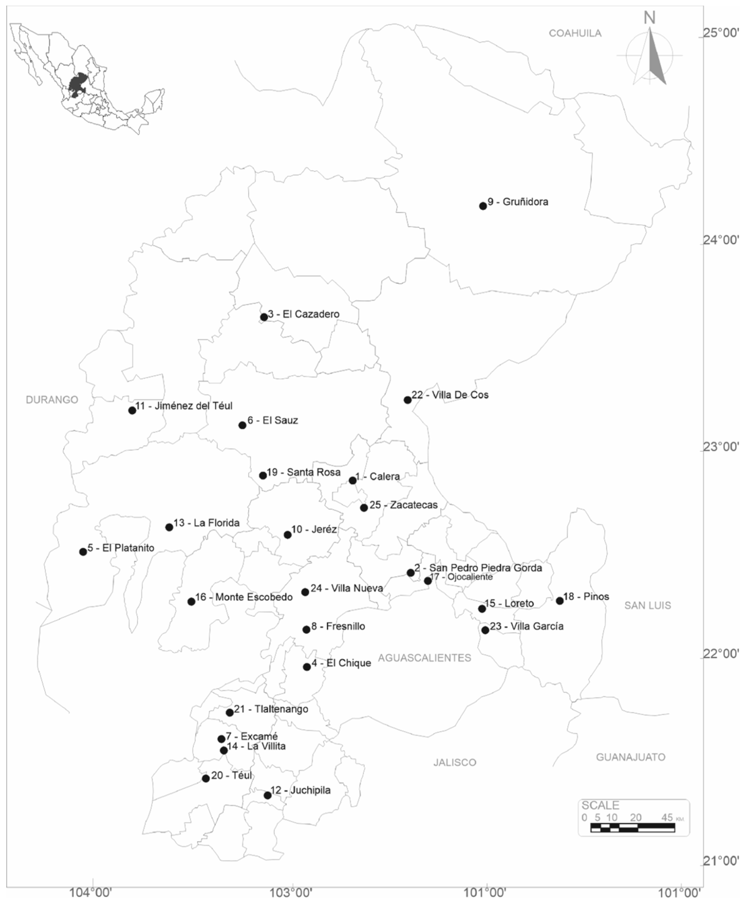
2.1. Data

In order to train the ANN models, a set of 6 input or predictor variables accompanied by a covariate were employed. These variables were used to depict the climatic and geographic attributes of weather stations established within the region of Zacatecas state in Mexico (Figure 1). The input or predictor variables were specific to each site and included the station ID, date, rainfall (PP), evaporation (EVP), maximum temperature (TMAX), minimum temperature (TMIN), and mean temperature (TMED). The evapotranspiration predictor (PET) was assessed using the Thornthwaite method [19]. The Multivariate El Niño Southern Oscillation Index v.2 (MEI) was later incorporated as a regression covariate during the training process of the ANN models.
Because the MEI database only has records dating back to 1979, this study exclusively considered weather stations with complete records from that year onwards as predictors or variables of interest. Therefore, a total of 24 weather stations were chosen for this study, with records spanning from 1979 to 2020. The input variables were acquired from a long-term meteorological dataset provided by the Mexican ‘Comisión Nacional del Agua’. Prior to any processing, the database underwent scrutiny to ensure the absence of any abnormal or missing data.

2.2. Standardized Precipitation Index

The Standardized Precipitation Index (SPI) [5] is a well-established tool used to measure the severity of precipitation anomalies over different time scales. To monitor and evaluate the prevailing drought conditions, the SPI is extensively employed. The SPI uses only precipitation data to calculate a standardized value that represents the deviation of the current precipitation from the long-term average for a given location and time period. The computation of the standardized value involves dividing the deviation between the current precipitation and the long-term average by the standard deviation of the long-term precipitation. The final SPI result is a value that is expressed in units of standard deviations from the long-term mean.
The computed SPI values could be classified into categories based on their magnitude, with negative values indicating drier than average conditions and positive values indicating wetter than average conditions [5]. Table 1 displays the categorization of SPI values, ranging from “extremely drought” to “extremely wet”, as well as intermediate categories indicating moderate to severe drought or wet conditions.
It is worth mentioning that the SPI can be calculated using different time scales, ranging from a few months to several years, depending on the needs of the user or application. Smaller time scales prove to be beneficial in monitoring drought conditions of shorter duration, whereas larger time scales can capture long-term alterations in rainfall patterns. As highlighted by [20], the 3-month SPI value characterizes moisture conditions over short to medium terms, the 6-month SPI value indicates agricultural droughts, and the 12-month SPI value corresponds to droughts impacting water supply reservoir levels. In this study, we specifically calculated the SPI values using a 12-month timeframe.
Due to the labor-intensive nature of manually calculating SPI values, several computer programs have been developed to streamline the process and increase accessibility. In our research, we used the SPEI15 package 1.8.1 [21] within the R system version 4.3.1 [22] for SPI computation.

2.3. Cluster Analysis

Cluster analysis is a statistical technique used to categorize elements or variables by grouping them together based on their similarities. The primary objective is to maximize the similarity within each group, ensuring homogeneity, while simultaneously maximizing the dissimilarities between groups [23]. The application of this technique as a statistical tool has gained extensive usage in delineating homogeneous climatic regions by utilizing observed values of meteorological variables, as demonstrated in previous studies [23,24].
In this study, a tree clustering algorithm was applied to cluster the entire set of 24 monthly SPI time series, which corresponded to 24 weather stations. The purpose was to group these stations into regions that exhibited similar SPI (i.e., pp regime) values. Through the application of the clustering technique, based on the observed similarity in their SPI values (i.e., pp regime), the analysis led to the identification of four unique regions: Semi-desert region (Pinos and Villa García), Highlands region (Calera, Cuahutemoc, El Cazadero, Fresnillo, Jerez, Jiménez, Loreto, Ojocaliente, Santa Rosa, Villa de Cos, and Zacatecas), Mountains region (El Chique, El platanito, El Sáuz, La Florida, Monte Escobedo, and Villanueva), and Canyons region (Excamé, Gruñidora, Juchipila, Téul, and Tlaltenango). In this study, we used two R packages, hclust [22] and ape [25], for the cluster computation under the R system 4.3.1 [22].

2.4. Potential Evapotranspiration Index

The PET represents the maximum amount of water that could evaporate from a vegetation-covered surface if unlimited water were available. This includes the combined water loss from both evaporation and transpiration within a specific crop or ecosystem [26].
In this study, with the availability of solely monthly rainfall and temperature data, the widely adopted Thornthwaite PET method [19], was used following the guidelines established in [27]. In this research, the SPEI package [21] was utilized to compute the PET index using the R system version 4.3.1 [22]. The mentioned packages in this research and the R system can both be accessed through the Comprehensive R Archive Network https://www.cran.r-project.org/ (accessed on 15 May 2024).

2.5. Multivariate ENSO Index Data

El Niño Southern Oscillation (ENSO) is a natural large-scale climatic phenomenon that affects weather worldwide, particularly rainfall patterns. It is characterized by fluctuating ocean temperatures in the central and eastern equatorial Pacific, accompanied by atmospheric changes above. The Multivariate ENSO Index (MEI) is the result of a process of standardizing six atmospheric and oceanic variables associated with ENSO and employing Principal Component Analysis to identify prevailing patterns of variability and decrease data dimensionality. The resulting Principal Components are weighted and combined to create a single index that represents the overall strength of ENSO [28,29].
The Multivariate ENSO Index Version 2 is computed by the National Oceanic and Atmospheric Administration. In this research, the MEI.v2 database spanning from 1979 to 2020 was used as a regression covariate for training the ANN models. The MEI.v2 database is available at http://www.esrl.noaa.gov (accessed on 15 May 2024).

2.6. Linear Models for Time-Series Forecasting

Linear models have been used as the standard approach for time-series forecasting. Despite the availability of newer methods, many researchers continue to rely on these models due to their simplicity in implementation and ability to produce accurate predictions.
The most-used linear models include and are not limited to the Linear Regression model, Auto-Regressive model, Moving-Average model, Auto-regressive and Moving-Average Model, and the Auto-Regressive Integrated Moving-Average model [30].
It is worth mentioning that the linear models discussed previously are commonly applied in modeling linear stochastic systems and are suitable for analyzing time-series data that exhibit stationarity. Nevertheless, this could also be seen as one of their main limitations.

2.7. Machine Learning for Time-Series Forecasting

Deep learning is a subfield of machine learning that uses neural networks having multiple hidden layers to identify and extract relevant features from data. Deep learning has become increasingly popular for time-series forecasting because it can learn features and patterns in the data that may be difficult for traditional statistical models to detect.
Time-series forecasting using deep learning models often incorporates Recurrent Neural Networks (RNNs) or their variants like the Gated Recurrent Unit (GRU) or Long Short-Term Memory (LSTM) models. These models can address inherent challenges associated with time-series data such as the temporal dependences in the data and can learn long-term patterns and trends.

2.7.1. Recurrent Neural Network

Recurrent Neural Networks (RNNs) are artificial neural networks knows for their effectiveness in handling sequential data, including time-series data [31]. RNNs can remember previous inputs and use them to inform their predictions for future outputs. In brief, RNNs are ideal to capture the temporal complex dynamics of the time series.
In a basic RNN architecture, each time step in the time series corresponds to an input to the network. The RNN processes the input at each time step along with its internal state, producing an output and updating its state. Subsequently, the output obtained can be utilized to predict the next time step, and this iterative process continues.
One issue with basic RNNs is that they can suffer from vanishing gradients, which makes it difficult for the network to learn long-term dependencies. To overcome this obstacle, more sophisticated RNN architectures have been devised, including the Gated Recurrent Unit (GRU) and Long Short-Term Memory (LSTM).

2.7.2. Long Short-Term Memory

Long Short-Term Memory (LSTM) was introduced to address the problem of vanishing gradients that can occur in traditional RNNs. LSTM is particularly well-suited for time-series forecasting tasks [32].
Like other RNNs, LSTM was conceived with the aim to process sequential data, such as time-series data, by maintaining an internal state that is updated with each new input. Nevertheless, LSTM employs a more intricate internal structure compared to conventional RNNs, incorporating three gating mechanisms such as an input gate, forget gate, and output gate.
The input gate regulates the extent to which the new input is integrated into the present state, while the forget gate manages the degree to which the prior state is disregarded. Lastly, the output gate governs the proportion of the current state that should be emitted as the output.
Each gate is controlled by a sigmoid activation function that produces values between 0 and 1, allowing the network to selectively adjust the amount of information that is remembered or forgotten.
Alongside the gating mechanisms, LSTM incorporates a memory cell, enabling the network to retain information over long periods of time. The memory cell undergoes updates using information from the input gate, forget gate, and a candidate activation function. The candidate activation function calculates a new value for the memory cell by considering the previous memory cell value and the current input.
The final output of the LSTM at each time step is determined by a combination of the current hidden state and the memory cell. The hidden state is updated considering both the output gate and the candidate activation function.
In time-series forecasting tasks, the LSTM can be trained to future values prediction of a time series based solely on past observations. The network takes in a sequence of past observations and uses them to update its internal state. Subsequently, the ultimate hidden state and memory cell of the network are employed to forecast the subsequent value in the time series.

2.7.3. Gated Recurrent Unit

Gated Recurrent Unit (GRU) is an RNN architecture that demonstrates notable suitability for tasks involving time-series forecasting. GRU was proposed as a simpler and more efficient alternative to the LSTM architecture, which may be more computationally expensive [33].
Similar to other RNNs, GRU is designed to process sequential data, such as time-series data, by maintaining an internal state that is updated with each new input. However, unlike traditional RNNs, GRU uses gating mechanisms to selectively remember or forget information from previous time steps.
The basic GRU architecture includes the following two gates: the reset gate and the update gate. The reset gate controls how much of the previous state to forget, while the update gate controls how much of the new input to incorporate into the current state. The reset and update gates are controlled by sigmoid activation functions that produce values between 0 and 1, allowing the network to selectively adjust the amount of information that is remembered or forgotten.
Alongside to the reset and update gates, GRU also has a candidate activation function that calculates a new hidden state considering the previous state and the current input. The employed candidate activation function is a hyperbolic tangent function, generating values ranging from −1 to 1.
The output of the GRU at each time step is determined by a combination of the current hidden state and the input at that time step. The hidden state considers the reset and update gates, along with the candidate activation function.
In time-series forecasting, GRUs are capable of learning long-term dependencies between past observations and future values. The network takes in a sequence of past observations and uses them to update its internal state. Afterward, the final hidden state of the network is used to predict the next value in the time series.

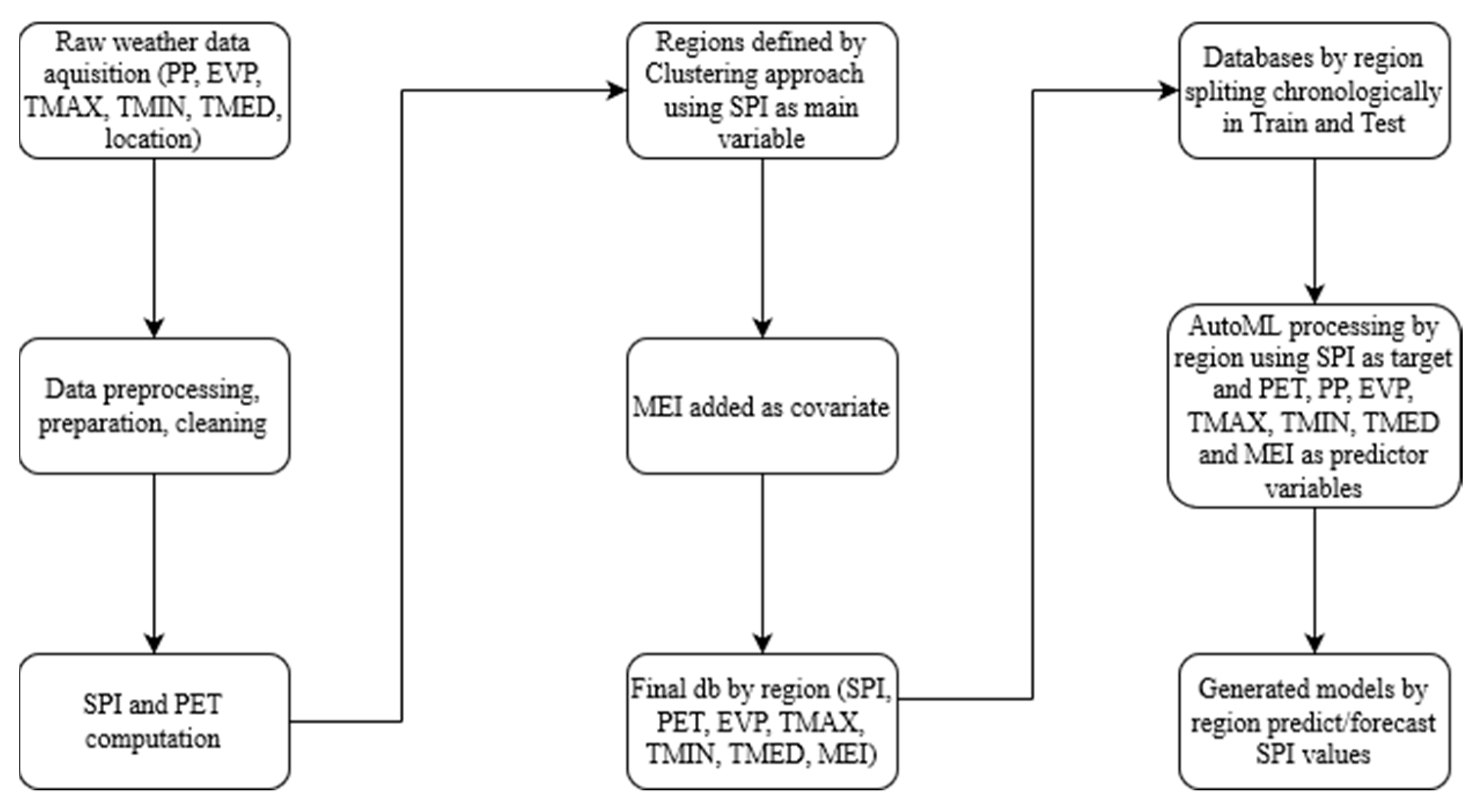
2.7.4. Automated Machine Learning

Automated Machine Learning is a process of automating the selection of the best models and their hyperparameters for a given task. It is a time-saving and cost-effective method for developing high-performance machine learning models with less human intervention [34]. AutoML for time-series prediction refers to the automated process of choosing the best models and hyperparameters for predicting future values of a time-series dataset.
Generally, the AutoML process for time-series prediction includes the following well-known steps:
  • Data preprocessing: This involves cleaning and preparing the time-series data for analysis, such as handling missing values, outliers, and converting the data into a suitable format for modeling.
  • Feature engineering: This step involves extracting relevant features from the time-series data to be used as input in the machine learning models.
  • Model selection: In this step, prediction of the forthcoming values of the time series is achieved by evaluating and comparing different machine learning models for their performance.
  • Hyperparameter tuning: This involves selecting the optimal values of hyperparameters for each machine learning model, which can significantly improve the model’s performance.
  • Ensemble learning: This step involves combining multiple machine learning models to improve the prediction accuracy of the time-series data.

2.7.5. AutoML Frameworks

AutoML for time-series prediction can be achieved using various platforms such as AutoGluon, AutoKeras, Auto-Pytorch, Auto-Sklearn, Auto-Weka, EvalML, H2O, TPOT, TransmogrifAI, TSPO, and many others [35]. These platforms automate the entire machine learning pipeline, from data preprocessing to model selection and deployment, making it easier for non-experts to develop accurate time-series prediction models.
We chose H2O AutoML [18] because is an open-source platform that outperformed Auto-Sklearn [34], TPOT [36], and AutoGluon [37] when using well-known public datasets [38].
H2O AutoML is a machine learning platform and AutoML module that encompasses various algorithms, including Random Forests, Extremely Randomized Trees, Generalized Linear Models (GLM), XGBoost, Gradient Boosting Machines (GBM), and Deep Neural Networks. Furthermore, it uses automated target encoding for high-dimensional categorical variables as a preprocessing technique [18].
H2O trains a randomized grid of algorithms by exploring a hyperparameter space. The individual models undergo tuning through cross-validation. Subsequently, the following two stacked ensembles are trained: one consisting of all models optimized for superior performance, and the other comprising only the best-performing model from each algorithm. The outcome is a sorted leaderboard showcasing all of the models [18].
In this analysis, H2O AutoML was selected to deploy individual neural network models to the cluster procedure results of the following four distinct regional time-series datasets: Semi-desert, Highlands, Mountains, and Canyons. The models were constructed using predictors such as the rainfall (PP), evaporation (EVP), maximum temperature (TMAX), minimum temperature (TMIN), mean temperature (TMED), evapotranspiration (PET), and MEI of the respective datasets from each region with the aim to forecast the SPI index values (i.e., target variable) specific to each region. Since the model was designed to forecast the SPI values that had already been normalized, there was no need to normalize or standardize the data again.
The consolidated dataset used for training each regional neural network consisted of a matrix comprising 504 timesteps (i.e., months) and 7 predictors, along with a vector representing the response variable over the same 504 timesteps (i.e., months). Table 2 displays a summary of descriptive statistics for the input predictors used to train the models.
When training multilayer networks, a common approach involves initially splitting the data into two distinct subsets. The initial subset is referred to as the training set and is utilized for computing the gradient as well as adjusting the weights and biases of the network. The second subset, known as the test set, is used to monitor the error throughout the training process. In the early stages of training, the test error usually decreases, mirroring the decline observed in the training set error.
The model architecture was constructed using the H2O AutoML platform, specifically version 3.40.0.2 [18], implemented with Python Language version 3.9.16 [39]. The training dataset for the model contained 80% of the available data in chronological order for each regional SPI time series (403 months spanning 1979 to 2007), while the remaining 20% was used for testing purposes (101 months spanning from 2007 to 2020).
A primary reason for using AutoML is its capability to automate the machine learning workflow. This includes automatically training and tuning the hyperparameters of different models, identifying a suitable model, and optimizing it [40]. When using H2O AutoML, besides the train and test databases, the only required parameters to run it were the name or index of the response variable (SPI) and the training frame or predictor variables (PP, EVP, TMAX, TMIN, TMED, PET, and MEI). Additionally required stopping parameters were provided separately; in this case, the maximum runtime of the AutoML process. No additional hyperparameters were required to run the AutoML. Optionally, it is possible to fine-tune several miscellaneous parameters [40]. The data flow processing is shown in Figure 2.

2.8. Performance Metrics

The assessment of the model’s performance relied on the use of widely recognized metrics and loss functions, including the Mean Squared Error (MSE) and Mean Absolute Error (MAE).
The Mean Squared Error (MSE) quantifies the difference between the actual and predicted values. A low MSE value signifies greater accuracy in the predictions.
M S E = 1 n i = 1 n S P I p i S P I o i 2
The Mean Absolute Error (MAE) measures the average absolute difference between the predicted and actual values of a variable.
M A E = 1 n i = 1 n S P I p i S P I o i
Alongside the MSE, the model’s goodness-of-fit was evaluated using the well-known R2 metric. The R2 metric measures the extent to which the model fits the data. Ideally, a perfect model (although improbable) would exhibit a low MSE, indicating minimal error accumulation, and high R2 values.
Lastly, the simple dissimilarity between the observed and predicted SPI values was employed to estimate the prediction error (PE) of the models.
P E = S P I o i S P I p i

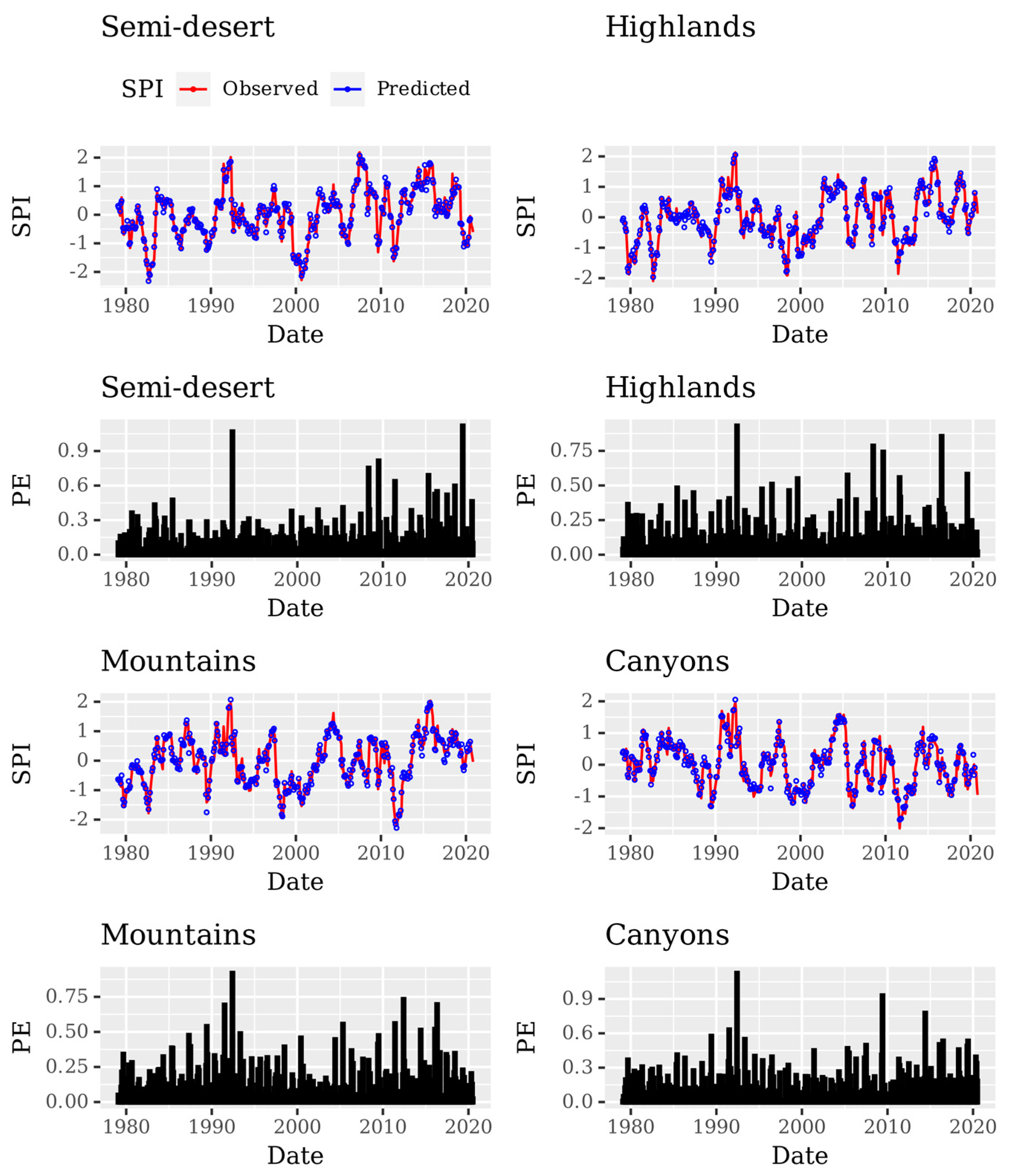
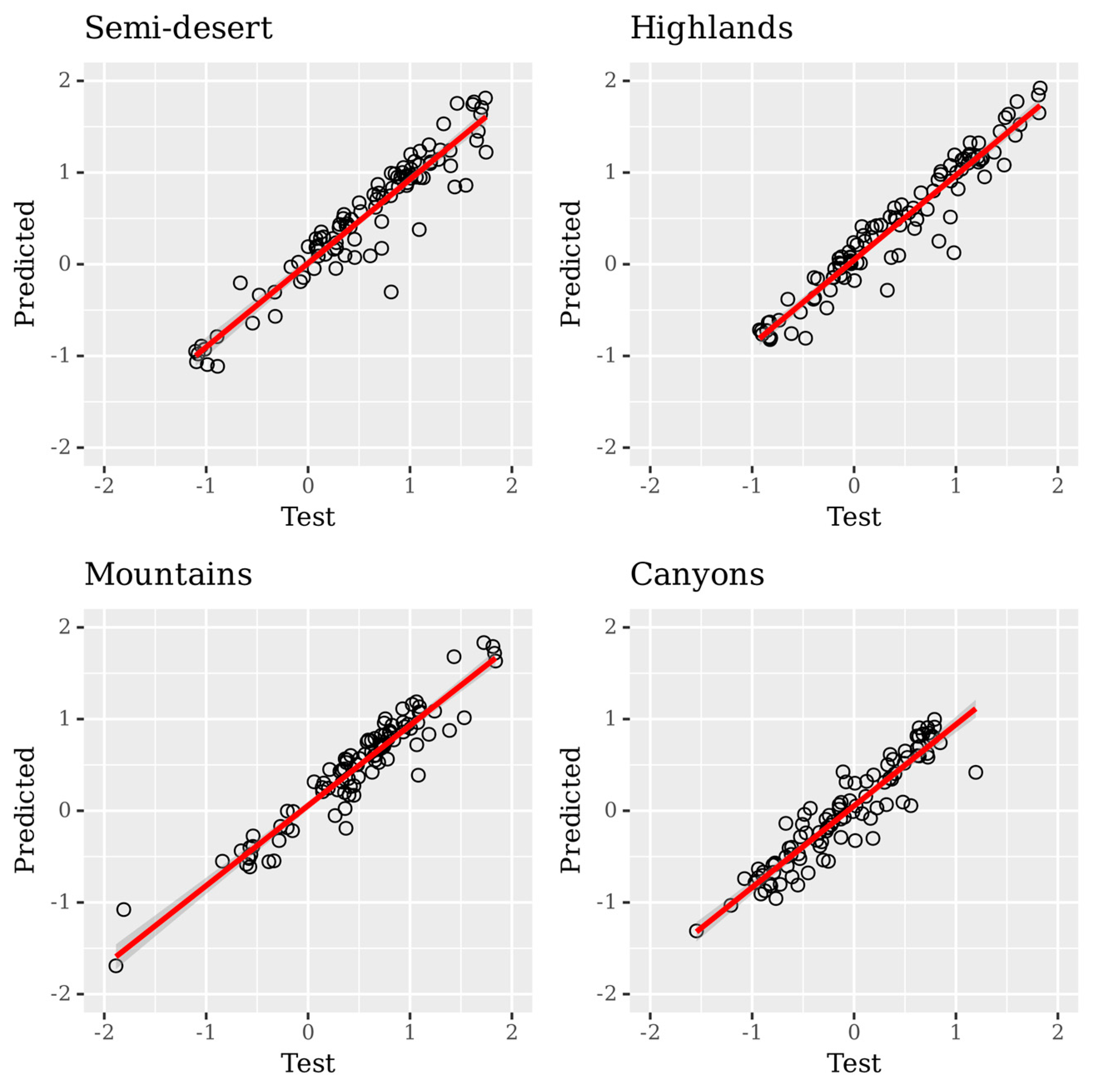
3. Results and Discussion

Figure 3 depicts the observed and predicted SPI time-series values alongside the Prediction Error for each region on the whole database (train and test) data. In general, the neural networks reported on the train data as well as cross-validation data using AutoML exhibited notable reductions in the MSE and MAE values, while showcasing high R2 values (Table 3).
The findings indicate that the performance of the SPI AutoML models across the four regions under study was considered satisfactory. H2O AutoML reported that, in the four analyzed regions, the models were obtained by means of stacked ensemble estimators with a cross-validation strategy and a GLM metalearner algorithm.
Overall, the comparison between the predicted and observed SPI values over the 100-month test period demonstrated a significant level of agreement, as shown in Figure 4. The statistical summary of the scatter plot, derived from linear regression analysis, illustrates the relationship between the predicted and observed SPI values for the test datasets. This summary is provided in Table 4 and further support the findings.
The evaluation of AutoML model’s performance involved assessing its ability to predict SPI values in the test datasets across all months. Performance metrics such as R2 and R values were used for comparison, as presented in Table 4.
Among the regions under consideration, AutoML models demonstrated the highest accuracy level in its predictions for the Highlands region, as indicated by the highest R value (0.964). The Mountains and Semi-desert regions showed the next best predictive performance, followed by the Canyons region with the lowest R value (0.933). However, overall, AutoML models demonstrated a satisfactory prediction skill for all regions considered in the study.
Table 5 provides a summary of the probability of prediction errors (PEs) under a normal distribution, indicating under-predictions (PE < 0) and over-predictions (PE > 0) made by AutoML models. A PE value of zero would signify a perfect alignment between the predicted and observed SPI values, indicating an ideal scenario [41]. Based on the findings, it is evident that AutoML models exhibited both under-prediction and over-prediction errors. Among the regions, the Canyons region displayed the most significant disparity, with a 62% likelihood of under-prediction. Likewise, over-prediction was noticed in the Semi-desert and Mountain regions, with the highest likelihood of over-prediction observed in the Semi-desert region (59.32%). These outcomes align with the summarized statistics of the linear models correlating the predicted and observed SPI values, as documented in Table 4.
Previous research has demonstrated the remarkable efficacy of neural networks in the empirical forecasting of hydrological variables [42,43,44,45]. Our findings are in line with the successful implementation of artificial neural network models in predicting the monthly standardized precipitation index, as evidenced by studies conducted by [4,15,16,46]. Moreover, our investigation aligns with the findings of [10], emphasizing the efficacy of the ANN network modeling technique in capturing the intricate nonlinear dynamics of complex systems, specifically in the domain of SPI time-series forecasting. Our results extend the findings of [8,9,17] by allowing the derivation of smaller and more detailed regional climatic zones in Mexico using the SPI. Furthermore, this study verifies that AutoML techniques are intended to independently identify suitable machine learning models and fine-tune them, facilitating effective optimization for time-series data forecasting [35]. In summary, our research findings demonstrated that the AutoML technique can be successfully used as a beneficial tool in the prediction of the SPI time series.

4. Conclusions

The incorporation of climatological variables such as rainfall, temperature, evaporation, and evapotranspiration into the machine learning models holds potential value for climate and water resource assessment. This integration allows for the comprehensive examination of these factors’ collective impact, thereby enabling the identification of climatic and agricultural risks.
Ensemble machine learning methods, along with deep learning methods, offer a means to attain exceptionally accurate forecasting time-series data. Particularly, AutoML can help overcome some of the challenges associated with developing and deploying ANNs for water resources and climate applications, making it a valuable tool for organizations looking to improve the accuracy and scalability of their models.
Future research on drought should focus on evaluation of several AutoML frame-works and compare their performance among them and against traditional machine learning methods to enhance the effectiveness of the deployed ANNs for drought indices prediction.

Author Contributions

Conceptualization, R.M.-Q.; Data curation, R.M.-Q.; Formal analysis, R.M.-Q. and C.E.G.-T.; Funding acquisition, H.G.-R.; Investigation, R.M.-Q., J.I.G.-T. and S.d.J.M.-G.; Methodology, R.M.-Q.; Project administration, R.M.-Q. and A.G.-D.; Resources, R.M.-Q.; Software, R.M.-Q. and J.I.G.-T.; Supervision, R.M.-Q.; Validation, R.M.-Q. and C.E.G.-T.; Visualization, R.M.-Q.; Writing—original draft, R.M.-Q.; Writing—review and editing, R.M.-Q. and A.G.-D. All authors have read and agreed to the published version of the manuscript.

Funding

This research received no external funding.

Data Availability Statement

The data used to support the findings of this study is called “Proyecto de bases de datos climatológicos”, and was supplied by the “Comisión Nacional del Agua”, the national official institution in charge of climatic and meteorological data record-keeping in Mexico. Data are available at: https://drive.google.com/drive/folders/10HCD7X_-sgTIJSQnJE9SkFL92ca3ERDC (accessed on 15 May 2024).

Conflicts of Interest

The authors declare no conflicts of interest.

References

  1. Kharin, V.V.; Zwiers, F.W.; Zhang, X.; Hegerl, G.C. Changes in Temperature and Precipitation Extremes in the IPCC Ensemble of Global Coupled Model Simulations. J. Clim. 2007, 20, 1419–1444. [Google Scholar] [CrossRef]
  2. Angheluță, P.S.; Badea, C.G. The Water Resources in the Context of Climate Change Produced by the Greenhouse Gases. Ann. Univ. Oradea 2015, 1, 637–643. [Google Scholar]
  3. Choubin, B.; Malekian, A.; Golshan, M. Application of Several Data-Driven Techniques to Predict a Standardized Precipitation Index. Atmosfera 2016, 29, 121–128. [Google Scholar] [CrossRef]
  4. Ali, Z.; Hussain, I.; Faisal, M.; Nazir, H.M.; Hussain, T.; Shad, M.Y.; Mohamd Shoukry, A.; Hussain Gani, S. Forecasting Drought Using Multilayer Perceptron Artificial Neural Network Model. Adv. Meteorol. 2017, 2017, 5681308. [Google Scholar] [CrossRef]
  5. McKee, T.B.; Doesken, N.J.; Kleist, J. The Relationship of Drought Frequency and Duration to Time Scales. In Proceedings of the 8th Conference on Applied Climatology, Anaheim, CA, USA, 17–22 January 1993; Volume 17, pp. 179–183. [Google Scholar]
  6. Naresh Kumar, M.; Murthy, C.S.; Sesha Sai, M.V.R.; Roy, P.S. On the Use of Standardized Precipitation Index (SPI) for Drought Intensity Assessment. Meteorol. Appl. 2009, 16, 381–389. [Google Scholar] [CrossRef]
  7. Mahfouz, P.; Mitri, G.; Jazi, M.; Karam, F. Investigating the Temporal Variability of the Standardized Precipitation Index in Lebanon. Climate 2016, 4, 27. [Google Scholar] [CrossRef]
  8. Giddings, L.; Soto, M.; Rutherford, B.M.; Maarouf, A. Standardized Precipitation Index Zones for México. Atmosfera 2005, 18, 33–56. [Google Scholar]
  9. Magallanes-Quintanar, R.; Blanco-Macías, F.; Galván-Tejada, E.C.; Galván-Tejada, J.; Márquez-Madrid, M.; Valdez-Cepeda, R.D. Negative Regional Standardized Precipitation Index Trends Prevail in the Mexico’s State of Zacatecas. Terra Latinoam. 2019, 37, 487–499. [Google Scholar] [CrossRef]
  10. Poornima, S.; Pushpalatha, M. Drought Prediction Based on SPI and SPEI with Varying Timescales Using LSTM Recurrent Neural Network. Soft Comput. 2019, 23, 8399–8412. [Google Scholar] [CrossRef]
  11. Chen, L.; Han, B.; Wang, X.; Zhao, J.; Yang, W.; Yang, Z. Machine Learning Methods in Weather and Climate Applications: A Survey. Appl. Sci. 2023, 13, 12019. [Google Scholar] [CrossRef]
  12. Ozger, M.; Mishra, A.K.; Singh, V.P. Estimating Palmer Drought Severity Index Using a Wavelet Fuzzy Logic Model Based on Meteorological Variables. Int. J. Climatol. 2011, 31, 2021–2032. [Google Scholar] [CrossRef]
  13. Masinde, M. Artificial Neural Networks Models for Predicting Effective Drought Index: Factoring Effects of Rainfall Variability. Mitig. Adapt. Strateg. Glob. Chang. 2014, 19, 1139–1162. [Google Scholar] [CrossRef]
  14. Belayneh, A.; Adamowski, J.; Khalil, B.; Ozga-Zielinski, B. Long-Term SPI Drought Forecasting in the Awash River Basin in Ethiopia Using Wavelet Neural Network and Wavelet Support Vector Regression Models. J. Hydrol. 2014, 508, 418–429. [Google Scholar] [CrossRef]
  15. Deo, R.C.; Şahin, M. Application of the Artificial Neural Network Model for Prediction of Monthly Standardized Precipitation and Evapotranspiration Index Using Hydrometeorological Parameters and Climate Indices in Eastern Australia. Atmos. Res. 2015, 161–162, 65–81. [Google Scholar] [CrossRef]
  16. Soh, Y.W.; Koo, C.H.; Huang, Y.F.; Fung, K.F. Application of Artificial Intelligence Models for the Prediction of Standardized Precipitation Evapotranspiration Index (SPEI) at Langat River Basin, Malaysia. Comput. Electron. Agric. 2018, 144, 164–173. [Google Scholar] [CrossRef]
  17. Magallanes-Quintanar, R.; Galván-Tejada, C.E.; Galvan-Tejada, J.I.; de Jesús Méndez-Gallegos, S.; Blanco-Macías, F.; Valdez-Cepeda, R.D. Artificial Neural Network Models for Prediction of Standardized Precipitation Index in Central Mexico. Agrociencia 2023, 57, 11–20. [Google Scholar] [CrossRef]
  18. LeDell, E.; Poirier, S. H2O AutoML: Scalable Automatic Machine Learning. In Proceedings of the 7th AutoML Workshop at ICML, San Diego, CA, USA, 17–18 July 2020; Volume 2020. [Google Scholar]
  19. Thornthwaite, C.W. An Approach toward a Rational Classification of Climate. Geogr. Rev. 1948, 38, 55–94. [Google Scholar] [CrossRef]
  20. Caloiero, T. Drought Analysis in New Zealand Using the Standardized Precipitation Index. Environ. Earth Sci. 2017, 76, 569. [Google Scholar] [CrossRef]
  21. Beguería, S.; Vicente-Serrano, S.M. SPEI: Calculation of the Standardized Precipitation-Evapotranspiration Index. In R Package Version 2017; R Foundation for Statistical Computing: Vienna, Austria, 2017; Volume 1. [Google Scholar]
  22. R Core Team. R: A Language and Environment for Statistical Computing; R Foundation for Statistical Computing: Vienna, Austria, 2013. [Google Scholar]
  23. Unal, Y.; Kindap, T.; Karaca, M. Redefining the Climate Zones of Turkey Using Cluster Analysis. Int. J. Climatol. 2003, 23, 1045–1055. [Google Scholar] [CrossRef]
  24. Karmalkar, A.V.; Bradley, R.S.; Diaz, H.F. Climate Change in Central America and Mexico: Regional Climate Model Validation and Climate Change Projections. Clim. Dyn. 2011, 37, 605–629. [Google Scholar] [CrossRef]
  25. Paradis, E.; Schliep, K. Ape 5.0: An Environment for Modern Phylogenetics and Evolutionary Analyses in R. Bioinformatics 2019, 35, 526–528. [Google Scholar] [CrossRef] [PubMed]
  26. Hanson, R.L. Evapotranspiration and Droughts. In National Water Summary 1988–89—Hydrologic Events and Floods and Droughts: US Geological Survey Water-Supply Paper; Le Haut Commissariat aux Eaux et Forêts: El Haj Kaddour, Morocco, 1991; Volume 2375. [Google Scholar]
  27. Vicente-Serrano, S.M.; Beguería, S.; López-Moreno, J.I. A Multiscalar Drought Index Sensitive to Global Warming: The Standardized Precipitation Evapotranspiration Index. J. Clim. 2010, 23, 1696–1718. [Google Scholar] [CrossRef]
  28. Wolter, K.; Timlin, M.S. Measuring the Strength of ENSO Events: How Does 1997/98 Rank? Weather 1998, 53, 315–324. [Google Scholar] [CrossRef]
  29. Wolter, K.; Timlin, M.S. El Niño/Southern Oscillation Behaviour since 1871 as Diagnosed in an Extended Multivariate ENSO Index (MEI.Ext). Int. J. Climatol. 2011, 31, 1074–1087. [Google Scholar] [CrossRef]
  30. Madsen, H. Time Series Analysis; Chapman and Hall/CRC: Boca Raton, FL, USA, 2007; ISBN 0-429-19583-4. [Google Scholar]
  31. Rumelhart, D.E.; Hinton, G.E.; Williams, R.J. Learning Representations by Back-Propagating Errors. Nature 1986, 323, 533–536. [Google Scholar] [CrossRef]
  32. Hochreiter, S.; Schmidhuber, J. Long Short-Term Memory. Neural Comput. 1997, 9, 1735–1780. [Google Scholar] [CrossRef] [PubMed]
  33. Cho, K.; Van Merriënboer, B.; Gulcehre, C.; Bahdanau, D.; Bougares, F.; Schwenk, H.; Bengio, Y. Learning Phrase Representations Using RNN Encoder-Decoder for Statistical Machine Translation. arXiv 2014, arXiv:1406.1078. [Google Scholar]
  34. Feurer, M.; Klein, A.; Eggensperger, K.; Springenberg, J.; Blum, M.; Hutter, F. Efficient and Robust Automated Machine Learning. Adv. Neural Inf. Process. Syst. 2015, 28, 2755–2763. [Google Scholar]
  35. Alsharef, A.; Aggarwal, K.; Kumar, M.; Mishra, A. Review of ML and AutoML Solutions to Forecast Time-Series Data. Arch. Comput. Methods Eng. 2022, 29, 5297–5311. [Google Scholar] [CrossRef]
  36. Olson, R.S.; Urbanowicz, R.J.; Andrews, P.C.; Lavender, N.A.; Kidd, L.C.; Moore, J.H. Automating Biomedical Data Science through Tree-Based Pipeline Optimization. In Proceedings of the 19th European Conference on the Applications of Evolutionary Computation, EvoApplications 2016, Porto, Portugal, 30 March–1 April 2016; Springer: Berlin/Heidelberg, Germany, 2016. Part I 19. pp. 123–137. [Google Scholar]
  37. Erickson, N.; Mueller, J.; Shirkov, A.; Zhang, H.; Larroy, P.; Li, M.; Smola, A. Autogluon-Tabular: Robust and Accurate Automl for Structured Data. arXiv 2020, arXiv:2003.06505. [Google Scholar]
  38. Paldino, G.M.; De Stefani, J.; De Caro, F.; Bontempi, G. Does AutoML Outperform Naive Forecasting? Eng. Proc. 2021, 5, 36. [Google Scholar] [CrossRef]
  39. Van Rossum, G.; Drake, F.L. Introduction to Python 3: Python Documentation Manual Part 1; CreateSpace: Scotts Valley, CA, USA, 2009; ISBN 1-4414-1270-0. [Google Scholar]
  40. H2O AutoML: Automatic Machine Learning. Available online: https://docs.h2o.ai/h2o/latest-stable/h2o-docs/automl.html (accessed on 28 June 2024).
  41. Moustris, K.P.; Larissi, I.K.; Nastos, P.T.; Paliatsos, A.G. Precipitation Forecast Using Artificial Neural Networks in Specific Regions of Greece. Water Resour. Manag. 2011, 25, 1979–1993. [Google Scholar] [CrossRef]
  42. Daliakopoulos, I.N.; Coulibaly, P.; Tsanis, I.K. Groundwater Level Forecasting Using Artificial Neural Networks. J. Hydrol. 2005, 309, 229–240. [Google Scholar] [CrossRef]
  43. Farajzadeh, J.; Fakheri Fard, A.; Lotfi, S. Modeling of Monthly Rainfall and Runoff of Urmia Lake Basin Using “Feed-Forward Neural Network” and “Time Series Analysis” Model. Water Resour. Ind. 2014, 7–8, 38–48. [Google Scholar] [CrossRef]
  44. Snieder, E.; Shakir, R.; Khan, U.T. A Comprehensive Comparison of Four Input Variable Selection Methods for Artificial Neural Network Flow Forecasting Models. J. Hydrol. 2020, 583, 124299. [Google Scholar] [CrossRef]
  45. Sharma, P.; Singh, S.; Sharma, S.D. Artificial Neural Network Approach for Hydrologic River Flow Time Series Forecasting. Agric. Res. 2022, 11, 465–476. [Google Scholar] [CrossRef]
  46. Bouaziz, M.; Medhioub, E.; Csaplovisc, E. A Machine Learning Model for Drought Tracking and Forecasting Using Remote Precipitation Data and a Standardized Precipitation Index from Arid Regions. J. Arid Environ. 2021, 189, 104478. [Google Scholar] [CrossRef]
Figure 1. Study region of Zacatecas state within the Mexican territory.
Climate 12 00102 g001
Figure 2. Data flow processing.
Climate 12 00102 g002
Figure 3. The recorded, forecasted, and predicted error values using whole database (train and test) data for the regional SPI time series in the territory of Zacatecas state, Mexico.
Climate 12 00102 g003
Figure 4. Scatter plot and trend lines between observed and predicted SPI values using test data for regional SPI time series in Zacatecas state, Mexico.
Climate 12 00102 g004
Table 1. Ranges and categories of standardized precipitation index values.
SPI ValueCategory
≥2.0Extremely wet
1.5 to 1.99Severely wet
1.0 to 1.49Moderately wet
−0.99 to 0.99Near normal
−1.49 to −0.99Moderately drought
−1.99 to −1.49Severely drought
≤2.0Extremely drought
Table 2. Predictor’s descriptive statistics by region used to train the AutoML models.
RegionPredictors
Semi-AridPP (mm)EVP (mm)TMED (°C)TMIN (°C)TMAX (°C)PET (mm)
Min0.00 58.00 10.05 −6.00 21.00 25.19
Mean 38.89 160.17 16.37 4.25 28.41 63.92
Max 339.50 299.90 21.36 11.50 42.06 105.22
SD 45.08 50.79 2.68 4.14 2.83 20.96
HighlandsPP (mm)EVP (mm)TMED (°C)TMIN (°C)TMAX (°C)PET (mm)
Min 0.00 91.91 9.98 −10.91 23.47 23.656
Mean 37.63 167.84 16.67 3.39 29.24 66.64
Max 275.56 308.82 22.51 11.32 35.54 114.41
SD 42.42 48.13 3.25 5.02 2.68 25.42
MountainsPP (mm)EVP (mm)TMED (°C)TMIN (°C)TMAX (°C)PET (mm)
Min 0.00 81.27 11.31 −6.42 25.32 25.29
Mean 47.22 166.44 18.18 4.39 31.57 74.30
Max 295.42 308.95 24.73 12.70 39.00 144.71
SD 54.72 54.54 3.39 5.18 2.91 30.78
CanyonsPP (mm)EVP (mm)TMED (°C)TMIN (°C)TMAX (°C)PET (mm)
Min 0.00 83.28 11.35 −5.43 24.30 26.54
Mean 53.55 156.84 18.50 4.63 31.74 72.97
Max 331.46 285.04 25.56 13.10 39.30 139.98
SD 62.17 47.83 3.32 5.13 2.89 29.02
Table 3. Quantitative performance metrics of the ANN reporting on train data (T) and cross-validation (CV) data for regional SPI time series in Zacatecas state, Mexico. Key metrics include the Mean Squared Error (MSE), Mean Absolute Error (MAE), and Determination coefficient (R2).
RegionTCVTCVTCV
MSEMAER2
Semi-desert0.02960.06150.12140.17260.95840.9136
Highlands0.03450.05030.1270.15340.94260.9163
Mountains0.03480.05570.12770.16320.94680.9149
Canyons0.03880.05490.13550.16370.93420.9067
Table 4. Performance of the ANN models using the linear regression formula (SPIp = β0 + β1 SPIo) applied to the observed SPI values (SPIo) and predicted SPI values (SPIp) using test data during the test period for regional SPI time series in Zacatecas state, Mexico.
Regionβ0β1R2R
Semi-desert0.0460.9800.8970.947
Highlands−0.0201.0080.9300.964
Mountains−0.0201.0500.9230.961
Canyons−0.0660.9810.8710.933
Table 5. Likelihood of prediction error (PE) under normal distribution for observed SPI values (SPIo) and predicted SPI values (SPIp) using test data during the test period for regional SPI time-series in the state of Zacatecas, Mexico.
RegionPE < 0PE > 0
Semi-desert0.40680.5932
Highlands0.53390.4661
Mountains0.49000.5100
Canyons0.62000.3800
Disclaimer/Publisher’s Note: The statements, opinions and data contained in all publications are solely those of the individual author(s) and contributor(s) and not of MDPI and/or the editor(s). MDPI and/or the editor(s) disclaim responsibility for any injury to people or property resulting from any ideas, methods, instructions or products referred to in the content.

