Transformer Encoder Enhanced by an Adaptive Graph Convolutional Neural Network for Prediction of Aero-Engines’ Remaining Useful Life

Abstract

Accurate prediction of remaining useful life (RUL) plays a significant role in ensuring the safe flight of aircraft. With the recent rapid development of deep learning, there has been a growing trend towards more precise RUL prediction. However, while many current deep learning methods are capable of extracting spatial features—those along the sensor dimension—through convolutional kernels or fully connected layers, their extraction capacity is often limited due to the small scale of kernels and the high uncertainty associated with linear weights. Graph neural networks (GNNs), emerging as effective approaches for processing graph-structured data, explicitly consider the relationships between sensors. This is akin to imposing a constraint on the training process, thereby allowing the learned results to better approximate real-world situations. In order to address the challenge of GNNs in extracting temporal features, we augment our proposed framework for RUL prediction with a Transformer encoder, resulting in the adaptive graph convolutional transformer encoder (AGCTE). A case study using the C-MAPSS dataset is conducted to validate the effectiveness of our proposed model.

1. Introduction

Aero-engines are the core power component of aircraft and whether they operate normally will have a crucial effect on the safety of the flight. However, aero-engines work under harsh environments [1] and have numerous components, meaning their reliability limited, which both make them prone to failure. But when the failure can be anticipated, carrying out maintenance at unreasonable times leads to the waste of time and cost. Thus, how to make an accurate prediction of the occurrence time of failure, that is, the remaining useful life (RUL) of current components, is a significant issue that needs to be researched.

The methods of RUL prediction can be roughly divided into two categories, model-based and data-based [2]. Model-based methods [3,4] predict the RUL through analyzing the degradation processes, such as cracks, fatigue, and deformation [5], which requires sufficient research on the mechanism of the degradation processes. For aero-engine complex systems, it is not possible to fully analyze the degradation mechanism of every component or the whole system, so we can only resort to data-driven methods. With the fast development of sensor technologies, a great number of data from aero-engines can be acquired [6], making it possible to implement data-driven methods in industrial applications. And this may be another of the reasons why data-driven methods have been a hot topic in the RUL prediction field in recent years [1] in addition to the rapid advances in artificial intelligence.

Data driven methods can be further classified into machine learning methods and deep learning methods. Conventional machine learning methods, such as Bayesian belief networks [7], support vector regression [8], and the support vector machine [9], have achieved positive results but demand extensive efforts for manual pre-feature engineering [1]. On the contrary, deep learning (DL) methods could map the monitoring data with not much preprocessing, such as max–min normalization, directly into the RUL values, possessing the strengths of convenience, low application threshold, and generality to a certain extent. Common DL methods include convolutional neural network (CNN)-based, recurrent neural network (RNN)-based, auto-encoder (AE)-based, Transformer-based methods, and their combination. For example, Li et al. [10] proposed a deep CNN (DCNN) framework for the RUL prediction. Sayah et al. [11] combined deep long short-term memory networks (LSTM) with Gaussian mixture models (GMMs) and applied it to the RUL prediction of complex industrial system components. Chen et al. [12] proposed a quadratic function-based deep convolutional AE (DCAE) to construct health indicators (HIs) and found that the extracted indicators have more predictive power than those bulit from traditional methods. Kamei et al. [13] developed two predictive models, LSTM and the Transformer, to predict the RUL, combined with two decentralized federated learning (FL) algorithms and verified the performance of FL.

Although these methods achieved great success, they each have their own drawbacks. For the CNN-based and AE-based methods, they could extract spatial features through convolutional kernels and fully connected layers along the dimension of the sensor, as shown in Figure 1, but they lack the capacity to model time series changes. For RNN-based and transformer-based methods, they all have fully connected layers along the dimension of the sensor, thus possessing the ability to extract spatial features to a certain extent. Moreover, different from CNN-based and AE-based methods, they could model time series changes so better results may be achieved. Furthermore, compared with RNN-based methods, Transformer-based methods have the capacity to capture long time dependencies, so they may perform better than RNN-based methods when dealing with long time series data [13]. However, for extracting spatial features using fully connected layers, a problem exists, i.e., only the loss function is used to constrain the values of linear weights and the learned weights may not reflects the true relationships between sensors, leading to suboptimal results. Thus, to make our trained model better extract true relationships between sensors, some other methods need to be introduced.

Graph neural networks (GNNs) [14], emerging as a kind of effective deep learning method, are developed to deal with graph-structured data. As the sensors in aero-engines intercorrelate with each other, it forms a kind of natural graph-structured data, with the sensors as nodes and relationships as edges. GNNs take the relationships between nodes into account explicitly, equivalent to adding a constraint compared to a linear weight whose elements could take any value. So the learned results may have a better approximation to the true situations. But general GNNs could not model time series changes, so some researchers combined GNNs with RNN-based methods to perform RUL prediction. For example, Li et al. [15] proposed a directed acyclic graph (DAG) network that combines LSTM and a CNN to predict the RUL. Kong et al. [16] combined a graph attention network (GAT) and LSTM to develop a graph neural network (GNN)-based spatio-temporal fusion attention (STFA) approach. But these methods may not be suitable for extracting long time dependencies, which may lead to suboptimal results. Moreover, little research combined GNN with the Transformer, whose performance is better than RNN when we deal with long time series data, to make RUL prediction. Based on this research result, we propose a new method called the adaptive graph convolutional transformer encoder (AGCTE) using the graph convolutional network (GCN) [17] and the Transformer encoder.

In AGCTE, the GCN part is used to model the sensor relationships and helps capture spatial features. The Transformer part is used to model the long time series changes. As a result, both spatial and temporal features could be extracted.

The remainder of this paper is organized as follows. Section 2 presents the AGCTE model used in this paper. Section 3 gives the descriptions of the experiments. Results and some analysis are shown in Section 4. This paper is finally concluded in Section 5.

2. Methodology

In this section, we will elaborate on our proposed architecture, as illustrated in Figure 2. It mainly contains two parts, adaptive GCN layers and the Transformer encoder.

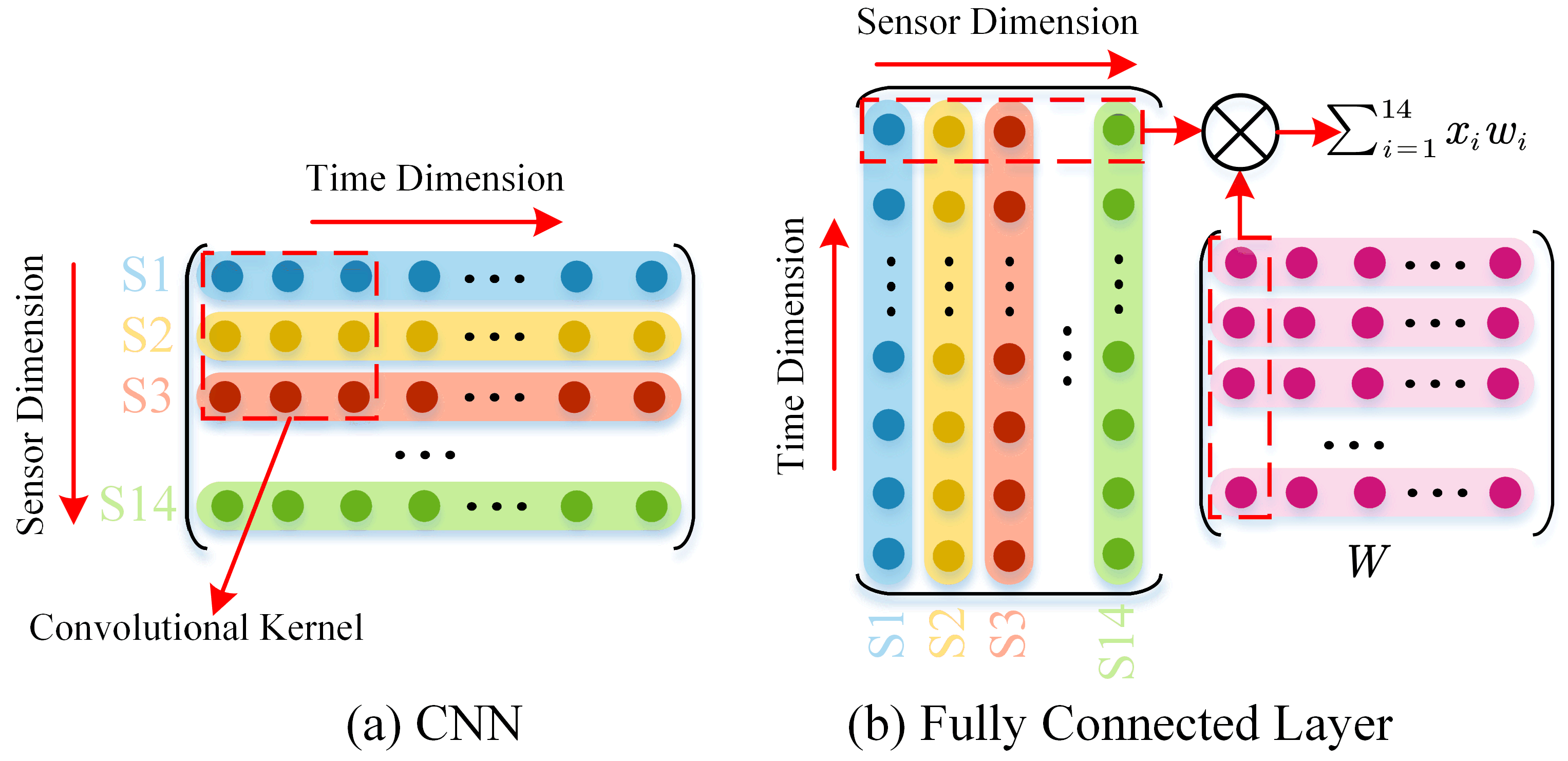
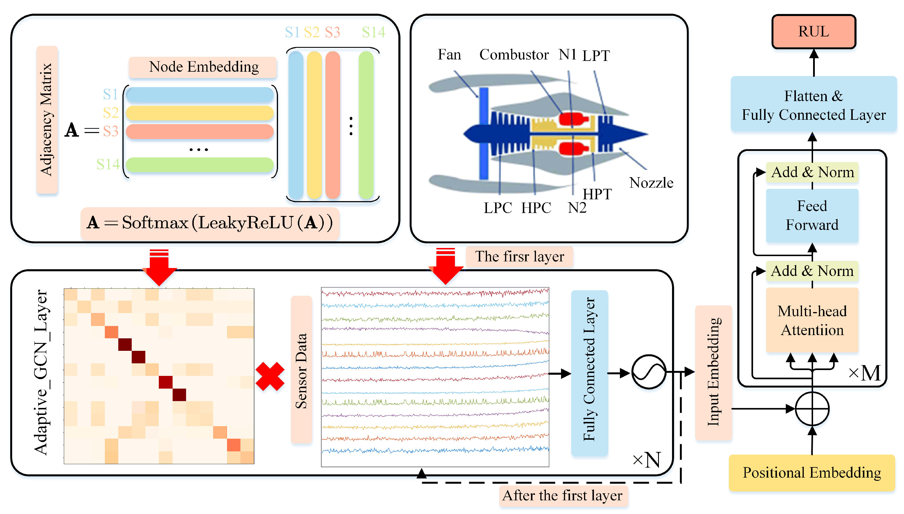
2.1. Adaptive GCN Layers

To use GCN, first, the adjacency matrix that describes the connection relationships between nodes should be defined. In some of the literature [6,17], a pre-defined graph is used, which is calculated as follows:

$$cos\theta =\frac{Cov({\mathbf{X}}_i,{\mathbf{X}}_j)}{{\sigma }_{{\mathbf{X}}_i}{\sigma }_{{\mathbf{X}}_j}}=\frac{E\left({\mathbf{X}}_i{\mathbf{X}}_j\right)-E\left({\mathbf{X}}_i\right)E\left({\mathbf{X}}_j\right)}{{\sigma }_{{\mathbf{X}}_i}{\sigma }_{{\mathbf{X}}_j}},$$

(1)

$${\mathbf{A}}_{ij}=\left\{\begin{array}{cc}cos\theta & ,cos\theta >0\\ 0& ,cos\theta <0\end{array}\right.,$$

(2)

where ${\mathbf{X}}_i$ and ${\mathbf{X}}_j$ are two 1-dimensional time series data; $E\left(·\right)$ means mathematical expectation function; ${\sigma }_{{\mathbf{X}}_i}$ and ${\sigma }_{{\mathbf{X}}_j}$ are the standard deviation of ${\mathbf{X}}_i$ and ${\mathbf{X}}_j$, respectively; and $cos\theta$ is the cosine similarity between ${\mathbf{X}}_i$ and ${\mathbf{X}}_j$. A problem exists in such a method: a predefined graph may not be best suitable for the GCN’s message passing process [18]. So in this paper, we use an adaptive generation approach. Following [19], we add a learnable embedding vector for every node, representing each sensor’s own characteristics:

$$\mathbf{V}={[{\mathbf{v}}_1^{\mathrm{T}},\dots ,{\mathbf{v}}_N^{\mathrm{T}}]}^{\mathrm{T}}\in {\mathrm{R}}^{N\times d},$$

(3)

where d represents the dimension of the embedding vector and N is the number of nodes. Then, following [20], we could acquire a learnable adjacency matrix using the following equation:

$$\mathbf{A}=Softmax\left(LeakyReLU(\mathbf{V}·{\mathbf{V}}^T)\right),$$

(4)

where Softmax is used to normalize the learned matrix and LeakyReLU is a non-linear activation function to enhance the learning capacity. Compared to the predefined graph, the adaptive graph is acquired during the process of training under the constraint of minimizing the loss function values. Thus, this graph may better serve the GCN’s message passing process. In classical GCN [21], the expression of GCN layer is as follows:

$$\mathbf{Y}=\sigma \left[\begin{array}{c}\widehat{\mathbf{A}}\mathbf{X}\mathbf{W}\end{array}\right],$$

(5)

where $\mathbf{Y}$ is the processed signal and $\mathbf{X}$ is the original signal; $\widehat{\mathbf{A}}={\tilde{\mathbf{D}}}^{-1/2}\tilde{\mathbf{A}}{\tilde{\mathbf{D}}}^{-1/2}$, $\tilde{\mathbf{A}}={\mathbf{A}}_0+\mathbf{I}$, and ${\mathbf{A}}_0$ is the adjacency matrix, $\mathbf{I}$ is the identity matrix, $\tilde{\mathbf{D}}$ is a diagonal matrix and its element ${\tilde{\mathbf{D}}}_{ii}={\sum }_{j=1}^N{\tilde{\mathbf{A}}}_{ij}$; $\mathbf{W}$ is the weight matrix; and $\sigma \left[·\right]$ is an activation function. In this paper, as Softmax function has already normalized the adjacency matrix, we use $\mathbf{A}$ to perform the message passing process and the adaptive GCN layer is as follows:

$$\mathbf{Y}=\sigma \left[\mathbf{A}\mathbf{X}\mathbf{W}\right].$$

(6)

2.2. Transformer Encoder

The Transformer is first proposed for natural language processing (NLP) in [22]. It consists of two parts, the encoder and decoder. Following the work in [23], we only use the encoder part to capture the short-term and long-term time series information. The encoder part is composed of input embedding, positional embedding, multi-head attention, skip connection, layer-normalization, and a feed-forward part. Their detailed descriptions are as follows.

2.2.1. Input Embedding

One of the functions of input embedding is to transform the dimension of the input to be suitable for the further calculation of multi-head attention. But the choice of the input embedding approaches, such as fully connected layer or CNN, could have a non-neligible effect on the final results. According to the experiments in [23], a fully connected layer could have a better processing effect than CNN, so in this paper, we take the same strategy and its expression is

$$\mathbf{Y}=\mathbf{Y}{\mathbf{W}}_i+{\mathbf{b}}_i,$$

(7)

where ${\mathbf{W}}_i$ is a learnable weight matrix and ${\mathbf{b}}_i$ is a learnable bias.

2.2.2. Positional Embedding

When multi-head attention is performed, unlike RNN-based methods, the sequential order of the input data loses. As a result, in order to keep such part of information, a positional embedding is added into the input after input embedding.

For a signal $\mathbf{Y}\in {\mathbb{R}}^{T\times D}$, where T is the time dimension and D is the feature dimension, first, a scaled factor $\sqrt{D}$ is used to enlarge the signal value to avoid the added positional embedding dominating the input. That is,

$$\mathbf{Y}=\mathbf{Y}·\sqrt{D}.$$

(8)

Then, the following positional embedding is added

$${\mathbf{p}}_{t,2d}=sin\left(t/{\mathrm{10,000}}^{2d/D}\right),$$

(9)

$${\mathbf{p}}_{t,2d+1}=cos\left(t/{\mathrm{10,000}}^{2d/D}\right),$$

(10)

$$\mathbf{Y}=\mathbf{Y}+\mathbf{p}.$$

(11)

2.2.3. Multi-Head Attention

Multi-head attention is composed of several parallel self-attention modules [24]. A self-attention function can be described as mapping a query and a set of key-value pairs to an output [22], where query, key, and value are the linear transformation of input, as

$${\mathbf{Q}}_i=\mathbf{Y}{\mathbf{W}}_i^q,$$

(12)

$${\mathbf{K}}_i=\mathbf{Y}{\mathbf{W}}_i^k,$$

(13)

$${\mathbf{V}}_i=\mathbf{Y}{\mathbf{W}}_i^v,$$

(14)

where ${\mathbf{W}}_i^q,{\mathbf{W}}_i^k,and {\mathbf{W}}_i^v\in {\mathbb{R}}^{D\times D_k}$ are learnable weight matrixes and ${\mathbf{Q}}_i,{\mathbf{K}}_i, and {\mathbf{V}}_i$ are query, key, and value, respectively. Then, the attention value can be calculated as follows:

$$\mathrm{Attention}\left({\mathbf{Q}}_i,{\mathbf{K}}_i,{\mathbf{V}}_i\right)=\mathrm{Softmax}\left(\frac{{\mathbf{Q}}_i{\mathbf{K}}_i^{\mathrm{T}}}{\sqrt{D_k}}\right){\mathbf{V}}_i.$$

(15)

For multi-head attention, we need to repeat the above process h times, where h is the number of heads. To be specific,

$$\mathrm{MultiHead}\left(\mathbf{Q},\mathbf{K},\mathbf{V}\right)=\mathrm{Concat}\left({\mathrm{head}}_1,\dots ,{\mathrm{head}}_h\right){\mathbf{W}}^O,$$

(16)

where ${\mathrm{head}}_i=\mathrm{Attention}({\mathbf{Q}}_i,{\mathbf{K}}_i,{\mathbf{V}}_i),{\mathbf{W}}^O\in {\mathrm{R}}^{h{D}_k\times D_{\mathrm{model}}},D_{\mathrm{model}}=D_{k}h$.

2.2.4. Feed-Forward Function

After the multi-head attention module, there is a feed-forward function consisting of two linear maps in the Transformer encoder. In this paper, the activation function is chosen as the GeLU function and the expression of this part is

$$\mathbf{Y}=\mathrm{GeLU}\left(\mathbf{Y}{\mathbf{W}}_1+{\mathbf{b}}_1\right){\mathbf{W}}_2+{\mathbf{b}}_2,$$

(17)

where ${\mathbf{W}}_1\in {\mathbb{R}}^{D_{\mathrm{model}}\times D_1},{\mathbf{W}}_2\in {\mathbb{R}}^{D_1\times D_2},{\mathbf{b}}_1\in {\mathbb{R}}^{D_1},and{\mathbf{b}}_2\in {\mathbb{R}}^{D_2}.$ The most important reason why we use the GeLU function is that it performs better in the Transformer than the ReLU function in many tasks and it follows some of the same work [23,25].

2.2.5. Skip Connection and Layernormalization

Skip connection and layernormalization are added twice in a transformer encoder layer and their positions are shown in Figure 2. Skip connection proves to be quite significant in ensuring the output does not converge to rank-1 matrix, keeping the performance of the Transformer [26].

3. Experiment

In this section, we give the description of the validation dataset we use and the basic experiment setting. The main contents of this section are dataset description, data preprocessing, evaluation metrics, and main implementation details.

3.1. Dataset Description

The C-MAPSS (Commercial Modular Aero-Propulsion System Simulation) dataset [27] is utilized to validate the effectiveness of our proposed model, AGCTE. This datatset is an aero-engine operation datasets, composed of four subdatasets, FD001 to FD004. Each subdataset contains numerous aero-engines and has three files for training, whose data are of rul-to-failure kind, testing and corresponeding RUL values of testing set. The engines in the C-MAPSS dataset may work under different working conditions and have different failure modes. And there are 21 sensors recording the different operating parameters such as pressure and temperature. The detailed descriptions of the engines in C-MAPSS dataset and the sensors are list in

Table 1. The details of the engines in the dataset.

Dataset	FD001	FD002	FD003	FD004
Training EU	100	260	100	249
Testing EU	100	259	100	248
Working Conditions	1	6	1	6
Fault types	1	1	2	2

and

Table 2. The details of sensor measurement.

Number	Symbol	Description	Units
1	T2	Total temperature at fan inlet	°R
2	T24	Total temperature at LPC outlet	°R
3	T30	Total temperature at HPC outlet	°R
4	T50	Total temperature at LPT outlet	°R
5	P2	Pressure at fan inlet	psia
6	P15	Total pressure in bypass-duct	psia
7	P30	Total pressure at HPC outlet	psia
8	Nf	physical fan speed	rpm
9	Nc	physical core speed	rpm
10	epr	Engine pressure ratio (P50/P2)	-
11	Ps30	Static pressure at HPC outlet	psia
12	phi	Ratio of fuel flow to Ps30	pps/psi
13	NRf	Corrected fan speed	rpm
14	NRc	Corrected core speed	rpm
15	BPR	Bypass ratio	-
16	farB	Burner fuel-air ratio	-
17	htBleed	Bleed Enthalpy	-
18	Nf_dmd	Demanded fan speed	rpm
19	PCNfR_dmd	Demanded corrected fan speed	rpm
20	W31	HPT coolant bleed	lbm/s
21	W32	LPT coolant bleed	lbm/s

, respectively.

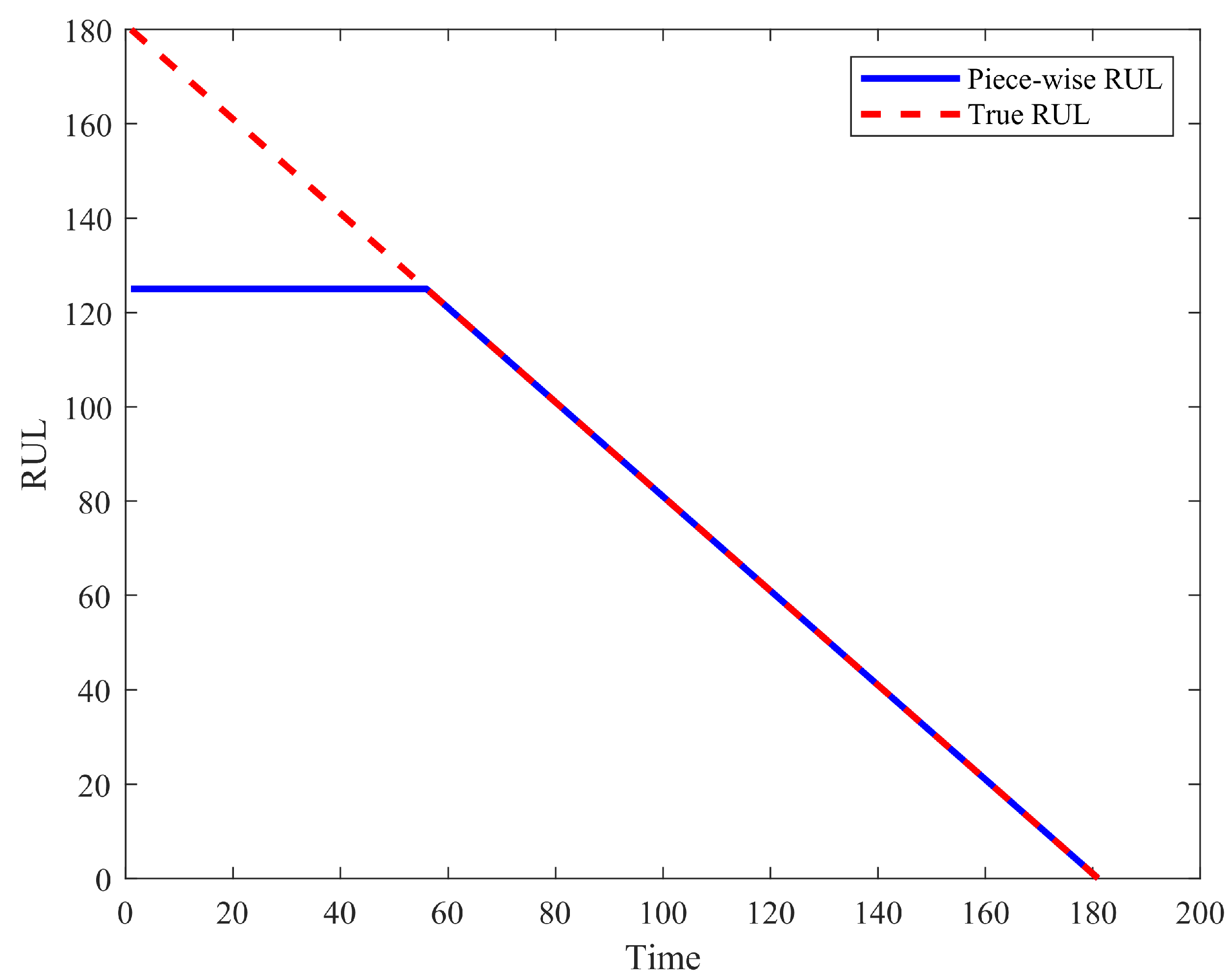
3.2. Data Preprocessing

There are 21 sensors available for our calculation. However, the values of seven of them do not change along with the time, which means they could not reflect the degradation process of the engines and are of no use for predicting the RUL. As a result, they are removed from the sensor list and the final chosen sensors are sensor 2, 3, 4, 7, 8, 9, 11, 12, 13, 14, 15, 17, 20, and 21.

After the sensor selection, the max–min normalization is performed to normalize each sensor data to [0, 1]. As the work conditions are multiple in FD002 and FD004 subdatasets, first K-means clustering is performed and then in each cluster class, the max–min normalization is utilized as follows:

$${\mathbf{y}}_{\mathrm{norm}}^{i,c}=\frac{{\mathbf{y}}^{i,c}-{\mathbf{y}}_{\min }^{i,c}}{{\mathbf{y}}_{\max }^{i,c}-{\mathbf{y}}_{\min }^{i,c}}$$

(18)

where ${\mathbf{y}}_{\mathrm{norm}}^{i,c}$ is the normalized sensor data; ${\mathbf{y}}^{i,c}$ is the original sensor data; and ${\mathbf{y}}_{max}^{i,c} and {\mathbf{y}}_{min}^{i,c}$ are the maximum and minimum of the i-th sensor under the c-th working condition, respectively. This calculation expression is also suitable for subdatasets FD001 and FD003.

Before training, in order to acquire more data samples, the sliding window method [23] is utilized to split the training set. Each slide forms a data sample and the goal is to predict the RUL of the next time after the end of this slide. Moreover, for RUL values used in model training, the maximum is set to 125 following previous research shown in Figure 3 [24] as at the initial operation stage of an engine, the degradation process is negligible so the RUL value could be considered as constant when we train our model for RUL prediction.

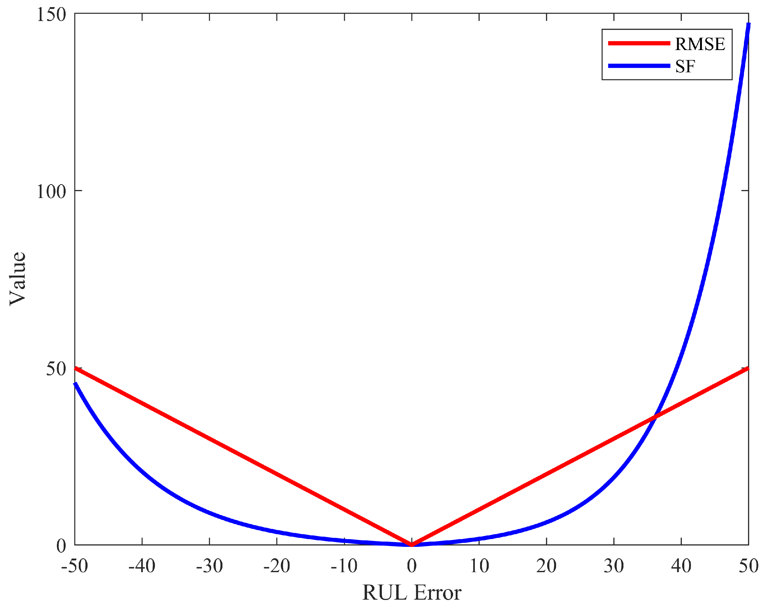
3.3. Evaluation Metrics

In this paper, two same evaluation metrics, root mean square error (RMSE) and scoring function (SF), are utilized to estimate the efficacy of the proposed model. RMSE and SF are defined as follows:

$${\delta }_i=\widehat{{\mathrm{RUL}}_i}-{\mathrm{RUL}}_i,$$

(19)

$$\mathrm{RMSE}=\sqrt{\frac{1}{|D_{\mathrm{test}}|}{\sum }_{i=1}^{|D_{\mathrm{test}}|}{\delta }_i^2},$$

(20)

$$\mathrm{SF}=\sum _{i=1}^{|D_{\mathrm{test}}|}{\mathrm{SF}}_i,\mathrm{with}{\mathrm{SF}}_i=\left\{\begin{array}{cc}{e}^{-{\delta }_i/13}-1\hfill & ,{\delta }_i<0\hfill \\ e^{{\delta }_i/10}-1\hfill & ,{\delta }_i>0\hfill \end{array}\right.,$$

(21)

where $\widehat{{\mathrm{RUL}}_i}$ and ${\mathrm{RUL}}_i$ are the predicted and ground-truth RUL of the i-th engine; $|D_{\mathrm{test}}|$ is the engine number of the testing set. The curves of RMSE and SF are plotted in Figure 4. The Score Function (SF) indicator was initially introduced in the PHM08 data competition and has since been widely utilized in remaining useful life (RUL) prediction to evaluate the performance of RUL models. Its significance can be elucidated as follows: when the predicted results deviate significantly from the actual RUL values, the resultant loss is substantial and the greater the disparity, the more pronounced the loss. Therefore, to mitigate such scenarios, the SF is formulated as an exponential function of the deviation, enabling the selection of models capable of minimizing substantial losses. Moreover, it is notable that there is a greater penalty imposed on predictions where the estimated RUL exceeds the actual RUL. This is because if the predicted RUL falls short of the actual RUL, it may not lead to catastrophic consequences, as appropriate maintenance measures could potentially extend the RUL. Conversely, if the predicted RUL surpasses the actual RUL, the situation is reversed. Consequently, predictions with an overestimation incur heavier penalties, reflecting the increased severity of such discrepancies.

3.4. Implementation Details

For the python library, our method is implemented in Pytorch. We use an Adam optimizer with 1 ×${10}^{-3}$ learning rate and set the number of adaptive GCN layers, Transformer encoder layers, and multi-head attention heads all to two. The feed-forward dimension in the Transformer encoder is set to 10. For FD001 and FD003, the model dimension of the Transformer encoder is set to 16, no dropout is used, and the activation function of adaptive GCN layers is tanh. While for FD002 and FD004, the model dimension of transformer encoder is set to 14, no activation function of adaptive GCN layers is used and dropout equals 0.2.

4. Results and Analysis

We compare our proposed model with 12 baselines, they are CNN-based methods [10,28], RNN-based methods [29,30], autoencoder-based methods [31], Transformer-based methods [13,24,32], and GNN-based methods [1,15,16,33]. The comparison results are listed in

Table 3. The RMSE experimental results of the C-MAPSS testing dataset.

Methods	FD001	FD002	FD003	FD004
CNN [28]	18.45	30.29	19.82	29.16	24.43
DCNN [10]	12.61	22.36	12.64	23.31	17.73
LSTM-FNN [29]	16.14	24.49	16.18	28.17	21.25
RBM-LSTM-FNN [30]	12.56	22.73	12.10	22.66	17.51
DSAE-TCN [31]	18.01	-	-	-	-
GCU-Transformer [24]	11.27	22.81	11.42	24.86	17.59
Transformer-1 [13]	13.52	16.11	17.10	19.77	16.63
Transformer-2 [32]	11.50	16.14	11.35	20.00	14.75
DAG [15]	11.96	20.34	12.46	22.43	16.80
STFA [16]	11.35	19.17	11.64	21.41	15.89
CDSG [1]	11.26	18.13	12.03	19.73	15.29
GGCN [33]	11.82	17.24	12.21	17.36	14.66
AGCTE (this paper)	12.46	13.7	12.95	15.83	13.74

and

Table 4. The SF experimental results of the C-MAPSS testing dataset.

Methods	FD001	FD002	FD003	FD004	Avg.
CNN [28]	1287	13,570	1596	7886	6084.75
DCNN [10]	274	10,412	284	12,466	5859
LSTM-FNN [29]	338	445	852	5550	2795.5
RBM-LSTM-FNN [30]	231	3366	251	2840	1672
DSAE-TCN [31]	161	-	-	-	-
GCU-Transformer [24]	-	-	-	-	-
Transformer-1 [13]	287.07	1436.74	263.64	2784.62	1193.02
Transformer-2 [32]	202	1131	227	2298	964.5
DAG [15]	229	2730	535	3370	1716
STFA [16]	194.44	2493.09	224.53	2760.13	1418.05
CDSG [1]	188	1740	218	2332	1119.5
GGCN [33]	186.6	1493.7	245.19	1371.5	824.25
AGCTE (this paper)	259.37	833.41	372.44	1520.05	746.32

.

From the results, it can be seen that our proposed model performs better than other methods in FD002 and FD004 subdatasets, especially for RMSE indicators. And in terms of both RMSE and SF indicators, the average performance of our model ranks first, demonstrating the effectiveness of our proposed model.

Moreover, four examples of the predicted RUL are depicted in Figure 5 and the comparison of the predicted RUL and the ground-truth RUL of the testing set of each subdataset are shown in Figure 6. From Figure 5, we can see that the error between the predicted RUL and the ground-truth RUL is relatively small in much of the time. In this phenomenon, our model could learn the linear degradation trend of aero-engines relatively well. From Figure 6, we can see that the run-to-failure prediction results are quite close to the ground-truth values, which is consistent with the results shown in Table 3 and Table 4 and demonstrates the effectiveness of our proposed model again.

In order to further verify the function of combining the GCN and Transformer encoder together, we perform an ablation study on our model, removing the GCN and Transformer encoder parts to form AGCTE-w/o GCN and AGCTE-w/o Transformer models, respectively. The RMSE of the experiments are listed in

Table 5. The RMSE of ablation study experiments.

Methods	FD001	FD002	FD003	FD004	Avg.
AGCTE	12.46	13.70	12.95	15.83	13.74
AGCTE-w/o GCN	13.6	14.16	12.86	16.36	14.26
difference	1.14	0.46	−0.09	0.53	0.51
AGCTE-w/o Transformer	13.27	22.83	12.73	35.94	21.19
difference	0.81	9.13	−0.22	20.11	7.76

.

From Table 5, it can be observed that average performances of the ablation models both have some decreases at different degrees, illustrating the effectiveness of combining GCN and the Transformer encoder together. Moreover, the performance of the model AGCTE-w/o Transformer decreases greatly, which demonstrates the significance of the Transformer encoder in RUL prediction. In addition, as depicted in Figure 1, the Transformer has fully connected layers along sensor dimension, thus possessing the capacity of extracting spatial features to a certain extent. But as we can see in Table 4, after adding the GCN part, the performance has certain improvements. This experiment result reveals that GCN can better extract spatial features that fully connect layers, as GCN takes the relationships between sensor explicitly. The learned adjacency matrixes are shown in Figure 7.

As for why our model performs better than other models on FD002 and FD004 subdatasets, we think the reasons can be two-fold. On one hand, we employ the normalization method tailored to different operating conditions, which will help reduce the effect that the variation in sensor values under different operating conditions has on the extraction of features related to the remaining using life (RUL) indicator. On the other hand, there has been one related work [23] purely using the Transformer encoder to perform RUL prediction on the same dataset. And we can see the results in [23]: the performance on FD002 and FD004 is better. Moreover, in ablation experiments, we can see AGCTE-w/o GCN, that is, the model only using the Transformer encoder, performs even better than our baselines on FD002 and FD004. Both results may demonstrate a conclusion that Transformer can better handle multiple operating condition data in RUL prediction. This may be attributed to the strong capacity of the Transformer to extract temporal features with no need to process time series data in sequence, as the data in multiple operating conditions could vary greatly point by point. And this may be another reason why our model performs better than other baselines. For the Transformer-1 and Transformer-2 method, there may be some slight differences from our model structure and setting. In the end, we found that the score value calculation equation in [23] is different from the popular setting, which is the reverse from that in [23]. So we think it may not be fair to compare our results with those in [23]. We foresee some small errors in their preprocessing code, which may also have unpredictable effects on the results.

5. Conclusions

In this paper, we propose a new model called AGCTE, which combines adaptive GCN and the transformer encoder together. The adaptive GCN part and the transformer encoder part are mainly utilized to extract spatial features and temporal features, respectively. The case study on the C-MAPSS dataset is carried out to validate the effectiveness of our proposed method. The results show the superiority of AGCTE compared with CNN-based, RNN-based, transformer-based, and GNN-based methods. In addition, the ablation study shows that combining GCN and transformer is reasonable and effective.

For further potential direction, as the current method extract spatial features and temporal features relatively independently using two separate modules, this may not be the most natural way to extract spatial–temporal features. As a result, developing a method that could extract spatial and temporal features at the same time may be the potential direction in the future.

References

1. Wang, H.; Zhang, Z.; Li, X.; Deng, X.; Jiang, W. Comprehensive Dynamic Structure Graph Neural Network for Aero-engine Remaining Useful Life Prediction. IEEE Trans. Instrum. Meas. 2023, 72, 3533816. [Google Scholar] [CrossRef]
2. Chen, J.; Shen, C.; Jing, Z.; Wu, Y.; Chen, R. Remaining useful life prediction of aircraft flap control system with mode transition. AIAA J. 2022, 60, 1104–1115. [Google Scholar] [CrossRef]
3. Wang, H.; Ma, X.; Zhao, Y. An improved Wiener process model with adaptive drift and diffusion for online remaining useful life prediction. Mech. Syst. Signal Proc. 2019, 127, 370–387. [Google Scholar] [CrossRef]
4. Chiachío, J.; Jalón, M.L.; Chiachío, M.; Kolios, A. A Markov chains prognostics framework for complex degradation processes. Reliab. Eng. Syst. Saf. 2020, 195, 106621. [Google Scholar] [CrossRef]
5. Li, Y.; Li, J.; Wang, H.; Liu, C.; Tan, J. Knowledge enhanced ensemble method for remaining useful life prediction under variable working conditions. Reliab. Eng. Syst. Saf. 2024, 242, 109748. [Google Scholar] [CrossRef]
6. Li, T.; Zhao, Z.; Sun, C.; Yan, R.; Chen, X. Hierarchical attention graph convolutional network to fuse multi-sensor signals for remaining useful life prediction. Reliab. Eng. Syst. Saf. 2021, 215, 107878. [Google Scholar] [CrossRef]
7. Zhang, X.; Kang, J.; Jin, T. Degradation modeling and maintenance decisions based on Bayesian belief networks. IEEE Trans. Reliab. 2014, 63, 620–633. [Google Scholar] [CrossRef]
8. Benkedjouh, T.; Medjaher, K.; Zerhouni, N.; Rechak, S. Health assessment and life prediction of cutting tools based on support vector regression. J. Intell. Manuf. 2015, 26, 213–223. [Google Scholar] [CrossRef]
9. Bezerra Souto Maior, C.; das Chagas Moura, M.; Didier Lins, I.; Lopez Droguett, E.; Henrique Lima Diniz, H. Remaining useful life estimation by empirical mode decomposition and support vector machine. IEEE Latin Am. Trans. 2016, 14, 4603–4610. [Google Scholar] [CrossRef]
10. Li, X.; Ding, Q.; Sun, J.-Q. Remaining useful life estimation in prognostics using deep convolution neural networks. Reliab. Eng. Syst. Saf. 2018, 172, 1–11. [Google Scholar] [CrossRef]
11. Sayah, M.; Guebli, D.; Noureddine, Z.; Al Masry, Z. Deep LSTM enhancement for RUL prediction using Gaussian mixture models. Autom. Control Comp. Sci. 2021, 55, 15–25. [Google Scholar] [CrossRef]
12. Chen, D.; Qin, Y.; Wang, Y.; Zhou, J. Health indicator construction by quadratic function-based deep convolutional auto-encoder and its application into bearing RUL prediction. ISA Trans. 2021, 114, 44–56. [Google Scholar] [CrossRef] [PubMed]
13. Kamei, S.; Taghipour, S. A comparison study of centralized and decentralized federated learning approaches utilizing the transformer architecture for estimating remaining useful life. Reliab. Eng. Syst. Saf. 2023, 233, 109130. [Google Scholar] [CrossRef]
14. Wu, Z.; Pan, S.; Chen, F.; Long, G.; Zhang, C.; Philip, S.Y. A comprehensive survey on graph neural networks. IEEE Trans. Neural Netw. Learn. Syst. 2020, 32, 4–24. [Google Scholar] [CrossRef] [PubMed]
15. Li, J.; Li, X.; He, D. A directed acyclic graph network combined with CNN and LSTM for remaining useful life prediction. IEEE Access 2019, 7, 75464–75475. [Google Scholar] [CrossRef]
16. Kong, Z.; Jin, X.; Xu, Z.; Zhang, B. Spatio-temporal fusion attention: A novel approach for remaining useful life prediction based on graph neural network. IEEE Trans. Instrum. Meas. 2022, 71, 1–12. [Google Scholar] [CrossRef]
17. Liu, N.; Guo, J.; Chen, S.; Zhang, X. Aero-Engines Remaining Useful Life Prognostics Based on Multi-Hierarchical Gated Recurrent Graph Convolutional Network. In Proceedings of the 2023 International Conference on Cyber-Physical Social Intelligence (ICCSI), Xi’an, China, 20–23 October 2023; pp. 642–647. [Google Scholar]
18. Gilmer, J.; Schoenholz, S.S.; Riley, P.F.; Vinyals, O.; Dahl, G.E. Neural message passing for quantum chemistry. In Proceedings of the International Conference on Machine Learning, Sydney, Australia, 6–11 August 2017; pp. 1263–1272. [Google Scholar]
19. Deng, A.; Hooi, B. Graph neural network-based anomaly detection in multivariate time series. In Proceedings of the AAAI Conference on Artificial Intelligence, Virtual, 2–9 February 2021; pp. 4027–4035. [Google Scholar]
20. Zhang, X.; Leng, Z.; Zhao, Z.; Li, M.; Yu, D.; Chen, X. Spatial-temporal dual-channel adaptive graph convolutional network for remaining useful life prediction with multi-sensor information fusion. Adv. Eng. Inform. 2023, 57, 102120. [Google Scholar] [CrossRef]
21. Kipf, T.N.; Welling, M. Semi-supervised classification with graph convolutional networks. arXiv 2016, arXiv:1609.02907. [Google Scholar]
22. Vaswani, A.; Shazeer, N.; Parmar, N.; Uszkoreit, J.; Jones, L.; Gomez, A.N.; Kaiser, Ł.; Polosukhin, I. Attention is all you need. Adv. Neural Inf. Process. Syst. 2017, 30. [Google Scholar]
23. Ogunfowora, O.; Najjaran, H. A Transformer-based Framework For Multi-variate Time Series: A Remaining Useful Life Prediction Use Case. arXiv 2023, arXiv:2308.09884. [Google Scholar]
24. Mo, Y.; Wu, Q.; Li, X.; Huang, B. Remaining useful life estimation via transformer encoder enhanced by a gated convolutional unit. J. Intell. Manuf. 2021, 32, 1997–2006. [Google Scholar] [CrossRef]
25. Devlin, J.; Chang, M.-W.; Lee, K.; Toutanova, K. Bert: Pre-training of deep bidirectional transformers for language understanding. arXiv 2018, arXiv:1810.04805. [Google Scholar]
26. Dong, Y.; Cordonnier, J.-B.; Loukas, A. Attention is not all you need: Pure attention loses rank doubly exponentially with depth. In Proceedings of the International Conference on Machine Learning, Virtual, 18–24 July 2021; pp. 2793–2803. [Google Scholar]
27. Saxena, A.; Goebel, K.; Simon, D.; Eklund, N. Damage propagation modeling for aircraft engine run-to-failure simulation. In Proceedings of the 2008 International Conference on Prognostics and Health Management, Denver, CO, USA, 6–9 October 2008; pp. 1–9. [Google Scholar]
28. Sateesh Babu, G.; Zhao, P.; Li, X.-L. Deep convolutional neural network based regression approach for estimation of remaining useful life. In Proceedings of the Database Systems for Advanced Applications: 21st International Conference, DASFAA 2016, Dallas, TX, USA, 16–19 April 2016; Proceedings, Part I 21. pp. 214–228. [Google Scholar]
29. Zheng, S.; Ristovski, K.; Farahat, A.; Gupta, C. Long short-term memory network for remaining useful life estimation. In Proceedings of the 2017 IEEE international conference on prognostics and health management (ICPHM), Dallas, TX, USA, 19–21 June 2017; pp. 88–95. [Google Scholar]
30. Ellefsen, A.L.; Bjørlykhaug, E.; Æsøy, V.; Ushakov, S.; Zhang, H. Remaining useful life predictions for turbofan engine degradation using semi-supervised deep architecture. Reliab. Eng. Syst. Saf. 2019, 183, 240–251. [Google Scholar] [CrossRef]
31. Liu, X.; Xiong, L.; Zhang, Y.; Luo, C. Remaining Useful Life Prediction for Turbofan Engine Using SAE-TCN Model. Aerospace 2023, 10, 715. [Google Scholar] [CrossRef]
32. Mo, H.; Iacca, G. Evolutionary neural architecture search on transformers for RUL prediction. Mater. Manuf. Process. 2023, 38, 1881–1898. [Google Scholar] [CrossRef]
33. Wang, L.; Cao, H.; Xu, H.; Liu, H. A gated graph convolutional network with multi-sensor signals for remaining useful life prediction. Knowl.-Based Syst. 2022, 252, 109340. [Google Scholar] [CrossRef]
Figure 1. The illustration of CNN and fully connected layer extracting spatial features.
Aerospace 11 00289 g001
Figure 2. Overall architecture of the proposed model.
Aerospace 11 00289 g002
Figure 3. Piece-wise RUL of the C-MAPSS dataset.
Aerospace 11 00289 g003
Figure 4. The curve of RMSE and SF.
Aerospace 11 00289 g004
Figure 5. Four examples of predicted RUL in the testing set.
Aerospace 11 00289 g005
Figure 6. Comparison of the predicted RUL and the ground-truth RUL of the testing set.
Aerospace 11 00289 g006
Figure 7. The learned adjacency matrixes in four subdatasets.
Aerospace 11 00289 g007