
Data Assimilation of Ideally Expanded Supersonic Jet Using RANS Simulation for High-Resolution PIV Data


Abstract
:1. Introduction
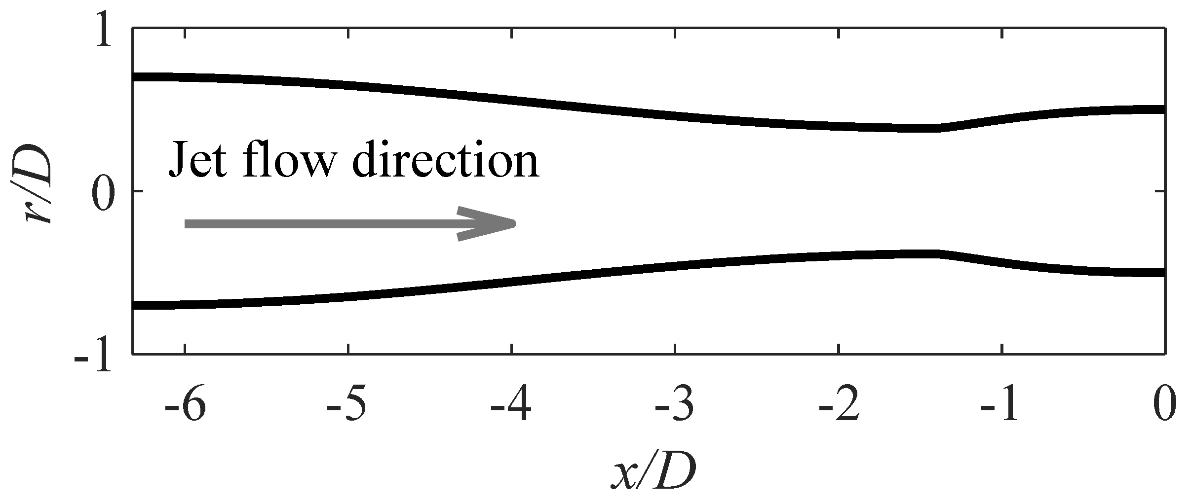
2. Jet Conditions
3. Methods
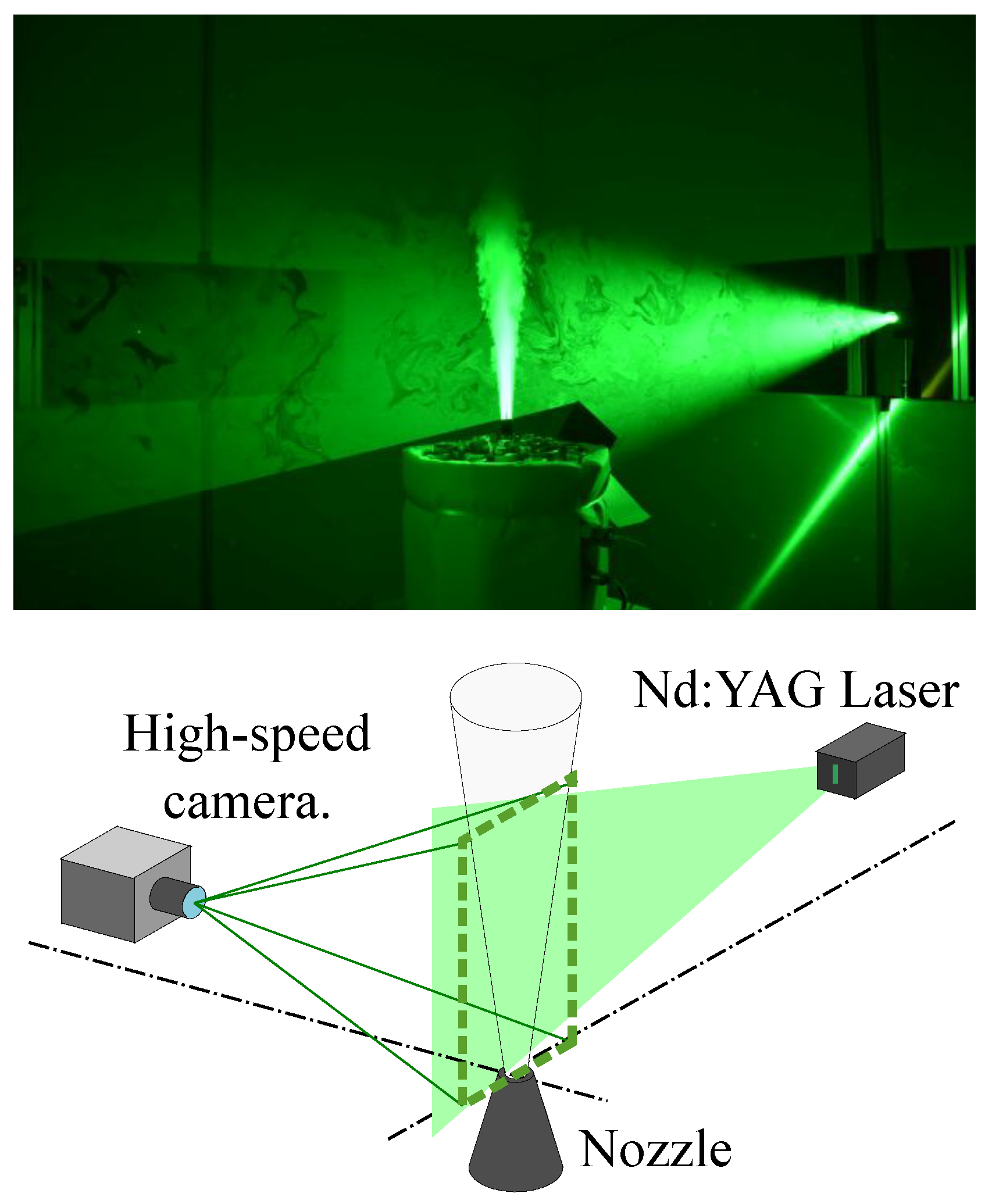
3.1. Experimental Apparatus
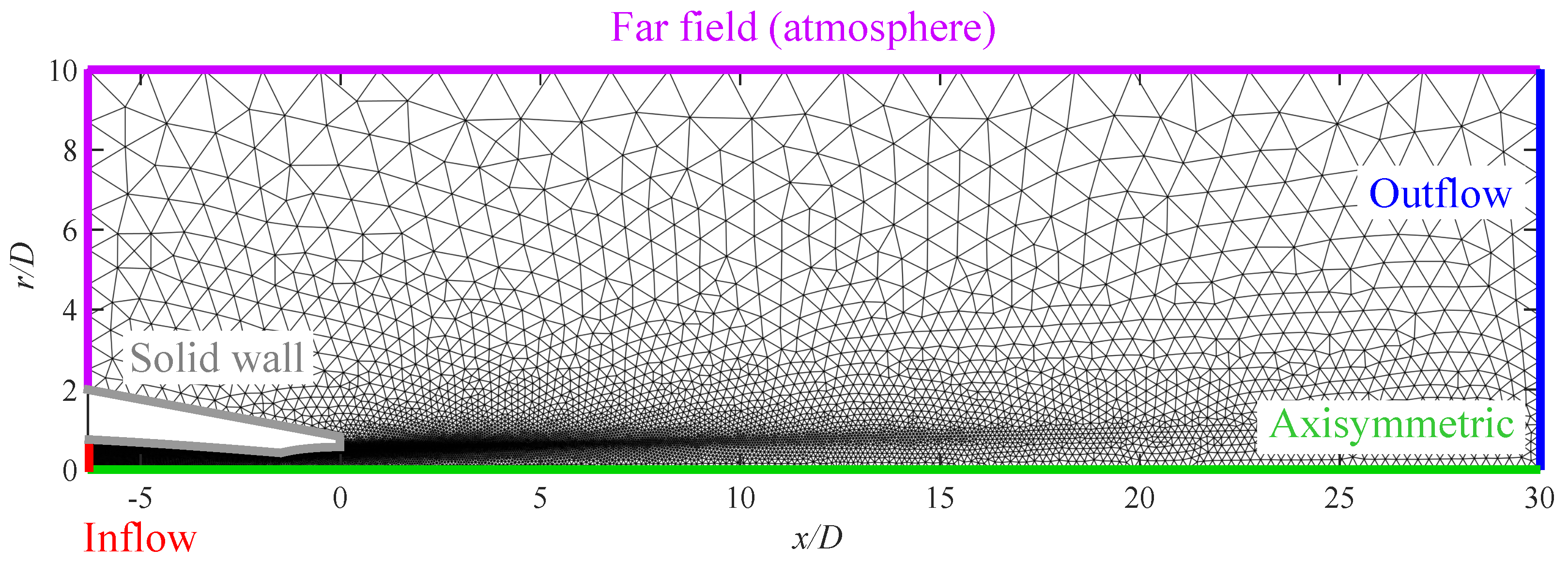
3.2. Numerical Apparatus
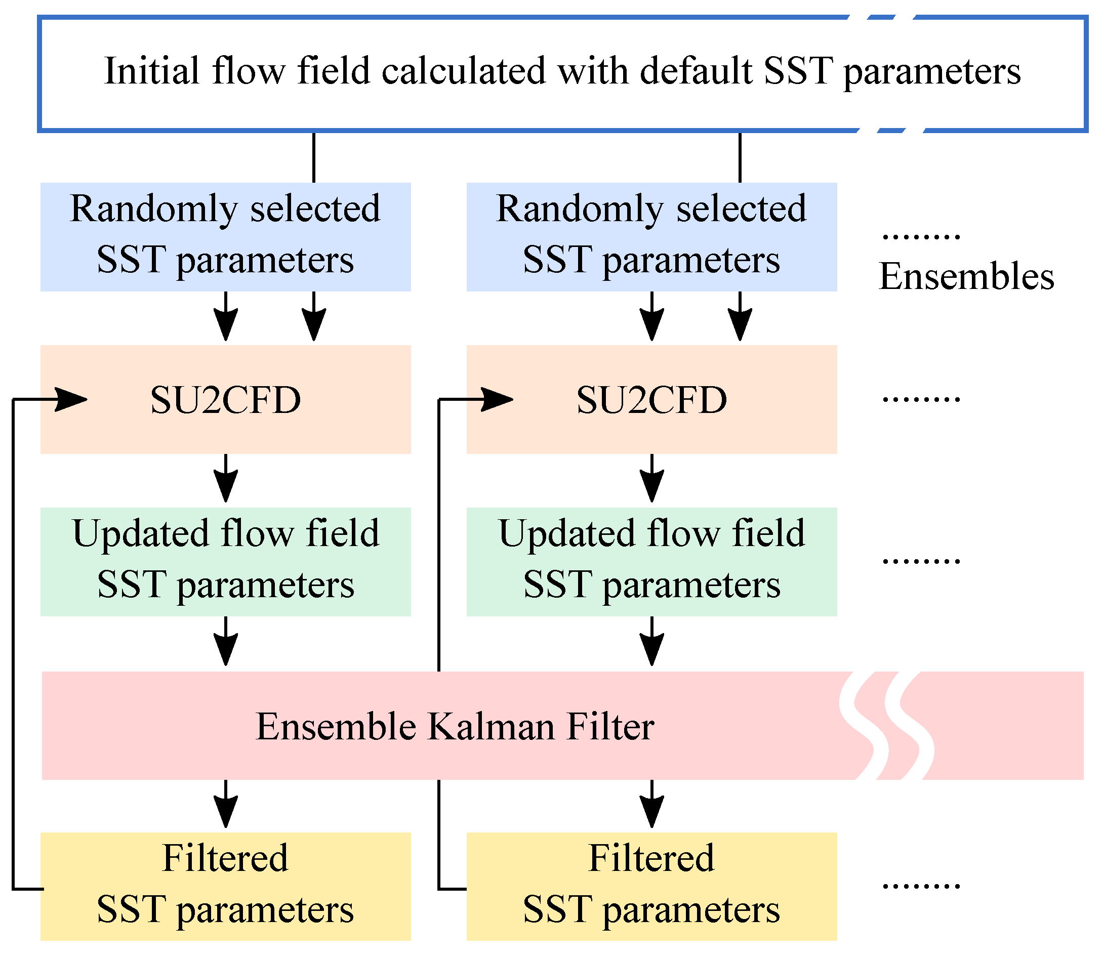
3.3. Data Assimilation
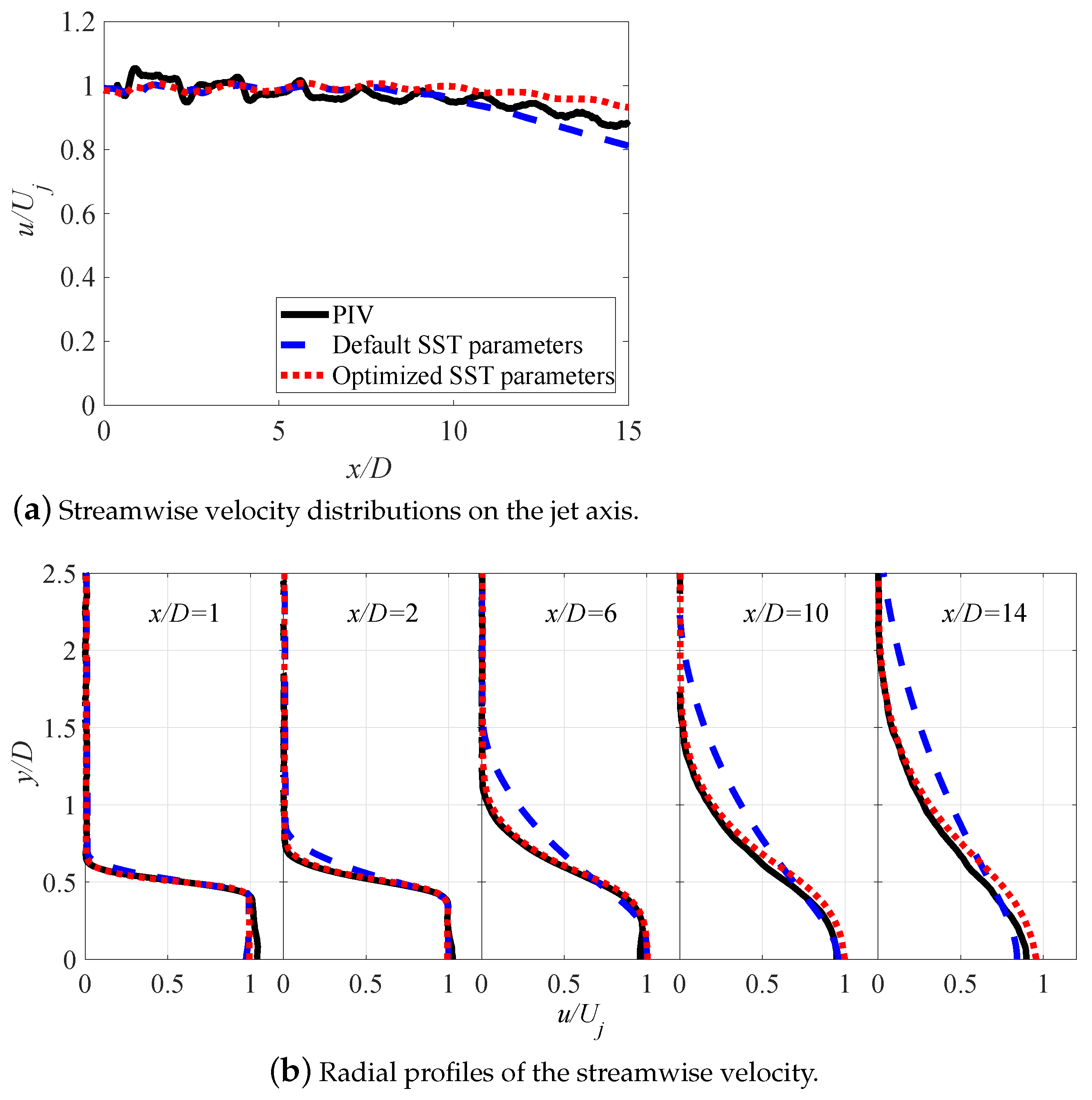
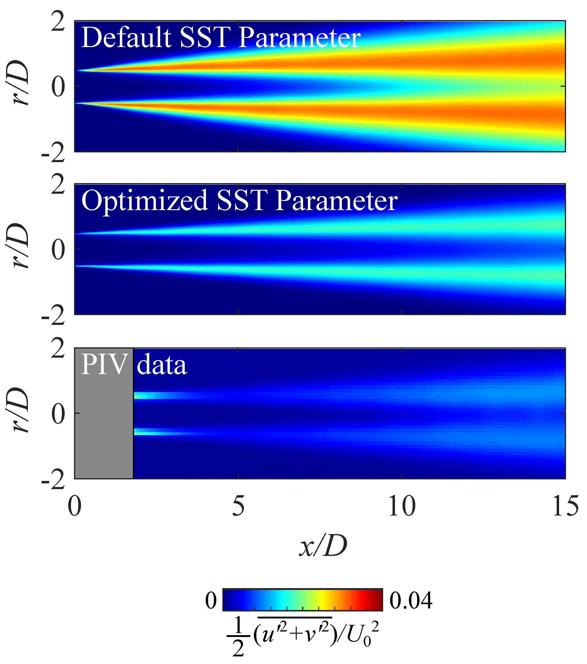
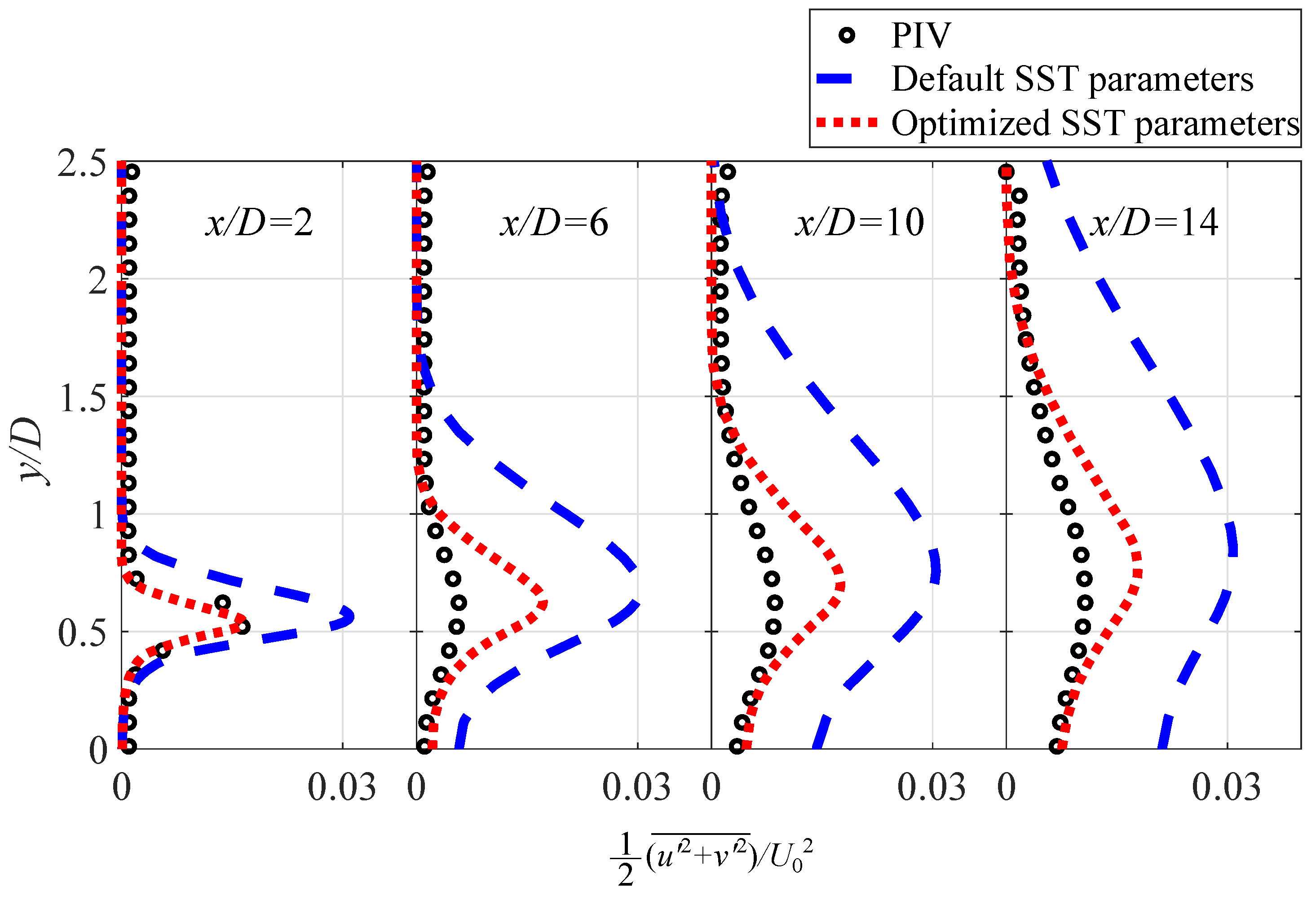
4. Results and Discussion
5. Conclusions
Author Contributions
Funding
Institutional Review Board Statement
Informed Consent Statement
Data Availability Statement
Conflicts of Interest
References
- Tam, C.K. Supersonic jet noise. Annu. Rev. Fluid Mech. 1995, 27, 17–43. [Google Scholar] [CrossRef]
- Raman, G. Supersonic jet screech: Half-century from Powell to the present. J. Sound Vib. 1999, 225, 543–571. [Google Scholar] [CrossRef]
- Bailly, C.; Fujii, K. High-speed jet noise. Mech. Eng. Rev. 2016, 3, 15-00496. [Google Scholar] [CrossRef]
- Brès, G.A.; Lele, S.K. Modelling of jet noise: A perspective from large-eddy simulations. Philos. Trans. R. Soc. A 2019, 377, 20190081. [Google Scholar] [CrossRef] [PubMed]
- Freund, J.; Colonius, T. Turbulence and sound-field POD analysis of a turbulent jet. Int. J. Aeroacoustics 2009, 8, 337–354. [Google Scholar] [CrossRef]
- Towne, A.; Schmidt, O.T.; Colonius, T. Spectral proper orthogonal decomposition and its relationship to dynamic mode decomposition and resolvent analysis. J. Fluid Mech. 2018, 847, 821–867. [Google Scholar] [CrossRef]
- McKeon, B.J.; Sharma, A.S. A critical-layer framework for turbulent pipe flow. J. Fluid Mech. 2010, 658, 336–382. [Google Scholar] [CrossRef]
- Jeun, J.; Nichols, J.W.; Jovanović, M.R. Input-output analysis of high-speed axisymmetric isothermal jet noise. Phys. Fluids 2016, 28, 047101. [Google Scholar] [CrossRef]
- Schmidt, O.T.; Towne, A.; Rigas, G.; Colonius, T.; Brès, G.A. Spectral analysis of jet turbulence. J. Fluid Mech. 2018, 855, 953–982. [Google Scholar] [CrossRef]
- Pickering, E.M.; Towne, A.; Jordan, P.; Colonius, T. Resolvent-based jet noise models: A projection approach. In Proceedings of the AIAA Scitech 2020 Forum, Orlando, FL, USA, 6–10 January 2020; p. 0999. [Google Scholar]
- Pickering, E.; Rigas, G.; Schmidt, O.T.; Sipp, D.; Colonius, T. Optimal eddy viscosity for resolvent-based models of coherent structures in turbulent jets. J. Fluid Mech. 2021, 917, A29. [Google Scholar] [CrossRef]
- Picard, C.; Delville, J. Pressure velocity coupling in a subsonic round jet. Int. J. Heat Fluid Flow 2000, 21, 359–364. [Google Scholar] [CrossRef]
- Tinney, C.; Ukeiley, L.; Glauser, M.N. Low-dimensional characteristics of a transonic jet. Part 2. Estimate and far-field prediction. J. Fluid Mech. 2008, 615, 53–92. [Google Scholar] [CrossRef]
- Ozawa, Y.; Nagata, T.; Nonomura, T. Spatiotemporal superresolution Measurement based on POD and Sparse Regression applied to a Supersonic Jet measured by PIV and Near-field Microphone. J. Vis. 2022; in press. [Google Scholar]
- Lee, C.; Ozawa, Y.; Nagata, T.; Nonomura, T. Super-resolution of time-resolved three-dimensional density fields of the B mode in an underexpanded screeching jet. Phys. Fluids 2023, 35, 065128. [Google Scholar]
- Ozawa, Y.; Honda, H.; Nonomura, T. Spatial superresolution based on simultaneous dual PIV measurement with different magnification. Exp. Fluids 2024, 65, 42. [Google Scholar] [CrossRef]
- Taira, K.; Brunton, S.L.; Dawson, S.T.; Rowley, C.W.; Colonius, T.; McKeon, B.J.; Schmidt, O.T.; Gordeyev, S.; Theofilis, V.; Ukeiley, L.S. Modal analysis of fluid flows: An overview. AIAA J. 2017, 55, 4013–4041. [Google Scholar] [CrossRef]
- Berkooz, G.; Holmes, P.; Lumley, J.L. The proper orthogonal decomposition in the analysis of turbulent flows. Annu. Rev. Fluid Mech. 1993, 25, 539–575. [Google Scholar] [CrossRef]
- Schmid, P.J. Dynamic mode decomposition of numerical and experimental data. J. Fluid Mech. 2010, 656, 5–28. [Google Scholar] [CrossRef]
- Tu, J.H.; Rowley, C.W.; Luchtenburg, D.M.; Brunton, S.L.; Kutz, J.N. On dynamic mode decomposition: Theory and applications. arXiv 2013, arXiv:1312.0041. [Google Scholar]
- Li, X.; Liu, N.; Hao, P.; Zhang, X.; He, F. Screech feedback loop and mode staging process of axisymmetric underexpanded jets. Exp. Therm. Fluid Sci. 2021, 122, 110323. [Google Scholar] [CrossRef]
- Rao, A.N.; Kushari, A.; Chandra Mandal, A. Screech characteristics of under-expanded high aspect ratio elliptic jet. Phys. Fluids 2020, 32, 076106. [Google Scholar] [CrossRef]
- Lim, H.; Wei, X.; Zang, B.; Vevek, U.; Mariani, R.; New, T.; Cui, Y. Short-time proper orthogonal decomposition of time-resolved schlieren images for transient jet screech characterization. Aerosp. Sci. Technol. 2020, 107, 106276. [Google Scholar] [CrossRef]
- Mercier, B.; Castelain, T.; Bailly, C. A schlieren and nearfield acoustic based experimental investigation of screech noise sources. In Proceedings of the 22nd AIAA/CEAS Aeroacoustics Conference, Lyon, France, 30 May–1 June 2016; p. 2799. [Google Scholar]
- Edgington-Mitchell, D.; Jaunet, V.; Jordan, P.; Towne, A.; Soria, J.; Honnery, D. Upstream-travelling acoustic jet modes as a closure mechanism for screech. J. Fluid Mech. 2018, 855, R1. [Google Scholar] [CrossRef]
- Tan, D.J.; Honnery, D.; Kalyan, A.; Gryazev, V.; Karabasov, S.A.; Edgington-Mitchell, D. Correlation analysis of high-resolution particle image velocimetry data of screeching jets. AIAA J. 2019, 57, 735–748. [Google Scholar] [CrossRef]
- Ozawa, Y.; Nonomura, T.; Oyama, A.; Asai, K. Effect of the Reynolds number on the aeroacoustic fields of a transitional supersonic jet. Phys. Fluids 2020, 32, 046108. [Google Scholar] [CrossRef]
- Lee, C.; Ozawa, Y.; Haga, T.; Nonomura, T.; Asai, K. Comparison of three-dimensional density distribution of numerical and experimental analysis for twin jets. J. Vis. 2021, 24, 1173–1188. [Google Scholar] [CrossRef]
- Price, T.J.; Gragston, M.; Kreth, P.A. Supersonic Underexpanded Jet Features Extracted from Modal Analyses of High-Speed Optical Diagnostics. AIAA J. 2021, 59, 4917–4934. [Google Scholar] [CrossRef]
- Davis, T.B.; Edstrand, A.; Cattafesta, L.N.; Alvi, F.S.; Yorita, D.; Asai, K. Investigation of the instabilities of supersonic impinging jets using unsteady pressure sensitive paint. In Proceedings of the 52nd Aerospace Sciences Meeting, National Harbor, MD, USA, 13–17 January 2014; p. 0881. [Google Scholar]
- Nonomura, T.; Nakano, H.; Ozawa, Y.; Terakado, D.; Yamamoto, M.; Fujii, K.; Oyama, A. Large eddy simulation of acoustic waves generated from a hot supersonic jet. Shock Waves 2019, 29, 1133–1154. [Google Scholar] [CrossRef]
- Nonomura, T.; Ozawa, Y.; Abe, Y.; Fujii, K. Computational study on aeroacoustic fields of a transitional supersonic jet. J. Acoust. Soc. Am. 2021, 149, 4484–4502. [Google Scholar] [CrossRef] [PubMed]
- Pineau, P.; Bogey, C. Links between steepened Mach waves and coherent structures for a supersonic jet. AIAA J. 2021, 59, 1673–1681. [Google Scholar] [CrossRef]
- Pineau, P.; Bogey, C. Numerical investigation of wave steepening and shock coalescence near a cold Mach 3 jet. J. Acoust. Soc. Am. 2021, 149, 357–370. [Google Scholar] [CrossRef]
- Semlitsch, B.; Mihăescu, M. Fluidic injection scenarios for shock pattern manipulation in exhausts. AIAA J. 2018, 56, 4640–4644. [Google Scholar] [CrossRef]
- Menter, F.R. Two-equation eddy-viscosity turbulence models for engineering applications. AIAA J. 1994, 32, 1598–1605. [Google Scholar] [CrossRef]
- Mishra, A.A.; Iaccarino, G. Uncertainty estimation for reynolds-averaged navier–stokes predictions of high-speed aircraft nozzle jets. AIAA J. 2017, 55, 3999–4004. [Google Scholar] [CrossRef]
- Mishra, A.A.; Mukhopadhaya, J.; Iaccarino, G.; Alonso, J. Uncertainty estimation module for turbulence model predictions in SU2. AIAA J. 2019, 57, 1066–1077. [Google Scholar] [CrossRef]
- Chauhan, M.; Massa, L. Stability Analysis of Thermally Nonuniform Supersonic Jets. AIAA J. 2020, 58, 5264–5279. [Google Scholar] [CrossRef]
- Bogey, C.; Bailly, C. Influence of nozzle-exit boundary-layer conditions on the flow and acoustic fields of initially laminar jets. J. Fluid Mech. 2010, 663, 507–538. [Google Scholar] [CrossRef]
- Kato, H.; Obayashi, S. Integration of CFD and wind tunnel by data assimilation. J. Fluid Sci. Technol. 2011, 6, 717–728. [Google Scholar] [CrossRef]
- Kato, H.; Yoshizawa, A.; Ueno, G.; Obayashi, S. A data assimilation methodology for reconstructing turbulent flows around aircraft. J. Comput. Phys. 2015, 283, 559–581. [Google Scholar] [CrossRef]
- Nakamura, M.; Ozawa, Y.; Nonomura, T. Low-Grid-Resolution-RANS-Based Data Assimilation of Time-Averaged Separated Flow Obtained by LES. Int. J. Comput. Fluid Dyn. 2022, 36, 167–185. [Google Scholar] [CrossRef]
- Deng, Z.; He, C.; Wen, X.; Liu, Y. Recovering turbulent flow field from local quantity measurement: Turbulence modeling using ensemble-Kalman-filter-based data assimilation. J. Vis. 2018, 21, 1043–1063. [Google Scholar] [CrossRef]
- He, X.; Yuan, C.; Gao, H.; Chen, Y.; Zhao, R. Calibration of Turbulent Model Constants Based on Experimental Data Assimilation: Numerical Prediction of Subsonic Jet Flow Characteristics. Sustainability 2023, 15, 10219. [Google Scholar] [CrossRef]
- Ozawa, Y.; Ibuki, T.; Nonomura, T.; Suzuki, K.; Komuro, A.; Ando, A.; Asai, K. Single-pixel resolution velocity/convection velocity field of a supersonic jet measured by particle/schlieren image velocimetry. Exp. Fluids 2020, 61, 129. [Google Scholar] [CrossRef]
- Westerweel, J.; Geelhoed, P.; Lindken, R. Single-pixel resolution ensemble correlation for micro-PIV applications. Exp. Fluids 2004, 37, 375–384. [Google Scholar] [CrossRef]
- Economon, T.D.; Palacios, F.; Copeland, S.R.; Lukaczyk, T.W.; Alonso, J.J. SU2: An open-source suite for multiphysics simulation and design. AIAA J. 2016, 54, 828–846. [Google Scholar] [CrossRef]
- Suzen, Y.; Hoffmann, K. Investigation of supersonic jet exhaust flow by one-and two-equation turbulence models. In Proceedings of the 36th AIAA Aerospace Sciences Meeting and Exhibit, Las Vegas, NV, USA, 24–28 July 1998; p. 322. [Google Scholar]
- Catris, S.; Aupoix, B. Density corrections for turbulence models. Aerosp. Sci. Technol. 2000, 4, 1–11. [Google Scholar] [CrossRef]
- Brown, J. Turbulence model validation for hypersonic flows. In Proceedings of the 8th AIAA/ASME Joint Thermophysics and Heat Transfer Conference, St. Louis, MI, USA, 24–26 June 2002; p. 3308. [Google Scholar]
- Gross, N.; Blaisdell, G.; Lyrintzis, A. Analysis of modified compressibility corrections for turbulence models. In Proceedings of the 49th AIAA Aerospace Sciences Meeting including the New Horizons Forum and Aerospace Exposition, Orlando, FL, USA, 4–7 January 2011; p. 279. [Google Scholar]


| Specifications of Laser: | |
| Laser system | LDY-300PIV (Litron) |
| Laser type | Nd:YLF |
| Laser wavelength | 527 nm |
| Pulse energy | 2 mJ at 10 kHz |
| Laser sheet width | approx. 0.8 mm |
| Specifications of Camera: | |
| High-speed camera | Phantom V611 (Vision Research) |
| Image sensor | pixels |
| Pixel pitch | 20 µm |
| Camera lens | Nikkor 80–200 mm f/2.8 |
| Measurement conditions: | |
| Measurement area | mm |
| Pixel resolution | pixels |
| Spatial discretization | 12.5 µm/pix |
| Time between laser pulses | 1.2 µs |
| Sampling rate | 1 kHz |
| Number of snapshots | 20,000 pairs |
| a | ||||||||
|---|---|---|---|---|---|---|---|---|
| 0.85 | 1.0 | 0.5 | 0.856 | 0.075 | 0.0828 | 0.09 | 0.31 | 0.41 |
| a | |||||||
|---|---|---|---|---|---|---|---|
| 0.474 | 0.574 | 0.393 | 0.634 | 0.070 | 0.102 | 0.080 | 0.434 |
Disclaimer/Publisher’s Note: The statements, opinions and data contained in all publications are solely those of the individual author(s) and contributor(s) and not of MDPI and/or the editor(s). MDPI and/or the editor(s) disclaim responsibility for any injury to people or property resulting from any ideas, methods, instructions or products referred to in the content. |
© 2024 by the authors. Licensee MDPI, Basel, Switzerland. This article is an open access article distributed under the terms and conditions of the Creative Commons Attribution (CC BY) license (https://creativecommons.org/licenses/by/4.0/).
Share and Cite
Ozawa, Y.; Nonomura, T. Data Assimilation of Ideally Expanded Supersonic Jet Using RANS Simulation for High-Resolution PIV Data. Aerospace 2024, 11, 291. https://doi.org/10.3390/aerospace11040291
Ozawa Y, Nonomura T. Data Assimilation of Ideally Expanded Supersonic Jet Using RANS Simulation for High-Resolution PIV Data. Aerospace. 2024; 11(4):291. https://doi.org/10.3390/aerospace11040291
Chicago/Turabian StyleOzawa, Yuta, and Taku Nonomura. 2024. "Data Assimilation of Ideally Expanded Supersonic Jet Using RANS Simulation for High-Resolution PIV Data" Aerospace 11, no. 4: 291. https://doi.org/10.3390/aerospace11040291