Abstract
A cold-gas test campaign has been conducted at the DLR’s P6.2 test bench in Lampoldshausen, with the objective of investigating the linear aerospike nozzle flow in interaction with secondary injection thrust vector control (SITVC). In this campaign, the influence of nozzle truncation, injection position and injection pressure on the nozzle surface and base pressure is analysed using pressure probes and Schlieren flow-visualisation techniques. The effects of injection position and truncation on the nozzle surface pressure development are comparable for all geometric variations, resulting in a locally increased static pressure upstream and a locally decreased static pressure downstream of the injection. The magnitude and dimension of these high- and low-pressure regions are correlated with the injection pressure. However, the influence of injection position and truncation on the base pressure is not entirely predictable by the named parameters, indicating an interdependence between both geometric parameters. Finally, the required pressure ratio of injection to the primary flow to ensure sonic injection has been analysed on TUD’s cold-gas test bench. This allows the respective injection position-dependent threshold to be identified. The analysis reveals that these experiments have been conducted under transsonic injection conditions.
1. Introduction
Aerospike nozzles represent a class of advanced nozzle concepts, offering a promising alternative to the conventional bell nozzles utilised in almost all launcher systems. They are well-known for their height-adaptive capabilities and additional performance potential compared to their bell nozzle counterparts [1,2,3,4,5]. The potential for replacing the F-1 engine in the Saturn V rocket (J-2T-250K) with an aerospike engine was discussed. Subsequently, this concept was considered for implementation as main engines for the Space Shuttle and for its successor, the Venture Star (XRS-2200) [6].
Despite the fact that aerospike engines were not deployed by any launch service provider yet, they have retained their appeal as a research topic in both academia and in the space industry. For instance, the students of the California Launch Vehicle Education Initiative (CALVEIN) [7] demonstrated the first successful flight of a bi-liquid-propelled aerospike rocket engine. On the other hand, the Dryden Aerospike Rocket Tests [8] yielded flight data for three solid-propelled high-power rockets utilising a conventional bell nozzle and two aerospike nozzles. However, the performance data for the aerospike engines did not demonstrate the anticipated performance benefits. Compared to the conventional nozzle counterpart, the aerospikes had lower combustion chamber pressure, correspondingly resulting in lower thrust. It was postulated that a larger throat area of the aerospike nozzles than the conventional ones might have been responsible for the discrepancy. In 2021, Pangea Aerospace [9] achieved stable combustion for a longer time in an annular aerospike engine operating on the propellants methane and liquid oxygen. This boosted the confidence in the possibility to deploy aerospike engines for practical application. In order to further enhance the application perspective, it is necessary to implement a method of thrust vector control (TVC). A literature review of Bach et al. [10] indicated secondary injection thrust vector control (SITVC) as a favourable solution for steering rockets and spacecrafts with aerospike nozzles, particularly for single-chambered engines. The utilisation of SITVC ceases the need for heavy gimballing and differential throttling.
To the best of our knowledge, aerospike engines with SITVC have been the subject of experimental research and development in the past by two main actors: Rocketdyne in the 1960s (as reported by Silver) and Eilers et al. in the 2010s (at Utah State University). Silver [11] reported 33 hot-fire tests, where the effects of thrust-vectoring in an annular aerospike nozzle for a variety of secondary injection positions and secondary mass flows were studied. He concluded that, for optimal performance of SITVC, a downstream injection position and higher mass flow rates were beneficial. On the other hand, in the MUPHyN project, Eilers et al. [12,13] conducted cold-flow experiments with three different secondary injection positions, where they evaluated the performance of side-force generation in terms of the side-specific impulse. Here too, they confirmed the performance advantage for a downstream injection position. Furthermore, the results demonstrated that, for equivalent mass flow ratios, a smaller orifice diameter for the injection was beneficial. Moreover, experimental evidence presented that the interaction of the main flow with the injection flow generated additional side-force components when compared to the secondary injection flow alone. This generation of additional side force was recently confirmed during the cold-gas experiments conducted at TUD, where the secondary injections were maintained at sonic speed for a geometric variety of injection orifices [14]. Additionally for linear nozzles, the optimal injection angle was observed to be slightly inclined towards the main flow. For both linear and annular nozzles, the optimal injection position was identified further downstream. However, no experimental data on the pressure distribution of linear or annular nozzles involving SITVC could be found.
The flow field and pressure distribution on linear aerospike nozzles with SITVC is considered analogous to the widely investigated canonical flow of a sonic jet in supersonic cross-flow over a flat plate. In this context, Spaid and Zukowski [15] conducted experimental analysis of the pressure field on the flat plate, where a high-pressure zone upstream and a low-pressure zone downstream of the injection were observed. They attributed these phenomena to the interaction of the jet and the cross-flow, where the two pressure zones exert a side force on the plate, together with the momentum flux of the jet, for which they derived an analytical formulation [16]. In contrast, as the cross-flow over an aerospike nozzle is accelerated rather than constant, the pressure distribution and corresponding side-force generation may behave differently.
In recent years, numerical simulations have been conducted by Propst et al. [17] and Ferlauto et al. [18] for linear aerospike nozzles with SITVC. Both analyses confirmed the comparable flow structure with the sonic jet in cross-flow situations, characterised by the high-pressure zone upstream and the low-pressure zone downstream of the injection. A preliminary verification of the simulations was conducted through shallow water experiments, which demonstrated the existence of the high-pressure zone in a qualitative manner [19,20]. However, an adequate quantitative measurement of the flow field could not be derived.
In order to address the paucity of experimental data, in summer 2019, a test campaign utilising two-dimensional, linear aerospike nozzles with SITVC was conducted in collaboration with the Flows Group of the Space Propulsion Institute in Lampoldshausen (German Aerospace Center, DLR). The experiments yielded comprehensive insights into the flow phenomena and pressure distribution on the nozzle and base surface. To the best of our knowledge, the data obtained represent the first experimental pressure data related to such flow conditions. In particular, the high-pressure region upstream and the low-pressure region downstream of the injection location could be experimentally verified.
Section 2 (Materials and Methods) provides a general overview of the experimental setup and specimen utilised in the presented investigation. It also presents the adaptability of the test specimen to test different truncation lengths and secondary injection (SI) positions. The surface and base pressure measurements are presented in Section 3 for all plugs in the two main flow conditions (under-expanded and over-expanded) with active SI. This is followed by a discussion and assessment of the results in Section 4.
2. Materials and Methods
The experimental setup was designed and realised for implementation at the DLR’s cold-gas test bench P6.2. In the following subsections, a general description of the test bench is provided, followed by a detailed explanation of the test specimen design. This section is concluded with the realisation of the test specimen. The presented description is an updated and shortened version of the preceding publication [21], which focused on the pre-test campaign held in December 2018. Further details are documented in [22].
2.1. Cold-Gas Test Bench P6.2
The cold-flow test facility P6.2 was implemented at the Space Propulsion Institute at Lampoldshausen in late 1998. The test facility provides up to three gaseous nitrogen (GN2) feeding lines, which can be pressure controlled separately. For the presented experiment, two out of three feed lines were used; one for the primary flow of the aerospike nozzle, expanding into ambient, and the other for secondary injection.
The fluidic interface for the test specimen was a rectangular flange of a Börger-contraction [23,24], with a flow cross-section of . Upstream, a diffuser and a flow straightener provided a homogeneous, rotation-free flow. In this location, the total pressure of the main flow was measured. The second feeding line for the secondary injection flow was realised with a corrugated metal hose having an inner diameter of , which was connected via a straight stainless steel tube with an inner diameter of . Two variations of a mounted test specimen with the feed lines are depicted in Figure 1.
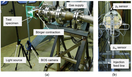
Figure 1.
Mounted test specimens and gas supply lines. (a) Aerospike nozzle with primary feed line and BOS setup [21]; (b) Aerospike nozzle with injection feed line and and pressure sensors—stern view.
The measurement interface was defined for the integration of the pressure sensors. Kulite® pressure transducers (Kulite, Leonia, NJ, USA) with pressure ranges of 0–0.1 … and a calibrated full-scale accuracy of were used. The sensors were directly connected to the test specimen via Teflon tubes.
In addition to the measurement of surface pressure, the visualisation of flow was a key aspect of this campaign. Two distinct flow-visualisation systems were employed for this purpose. The first one was a Z-Schlieren setup, which captured the flow in a perpendicular orientation to the two-dimensional nozzle plane, while the second system, a Background-Oriented Schlieren (BOS) system, captured the flow in a lateral orientation from within the aforementioned plane (see Figure 1). Both systems were capable of visualising changes in brightness caused by the deflection of light resulting from changes in the density gradient and, consequently, the refractive index of the flow. Consequently, they are well-suited to the detection of shocks and other flow phenomena that are to be expected in a supersonic flow.
2.2. Test Specimen Design
The test specimen and, in particular, the supersonic part of the nozzle were designed to fit the test-bench capabilities. These capabilities were limited to a maximum mass flow rate of and a maximum total pressure of [25,26,27]. The maximum throat area was calculated to be using and the gas properties for GN2 at room temperature.
An adaptation of the FORTRAN program of C. C. Lee [28] was used to obtain the normalised contour for linear aerospike nozzles based on the Prandtl–Meyer expansion. In order to derive a specific contour, further input parameters, such as the gas properties and the design pressure ratio, were required. The latter is defined as , the ratio of the total chamber pressure to the nozzle exit pressure . In this particular configuration, the nozzle expands to ambient pressure . Accordingly, is set equal to . Consequently, is constrained to ≈60, taking into account. In order to test all flow states from over-expanded and adapted to under-expanded , a slightly lower design pressure ratio of was chosen. Here, the nozzle pressure ratio was used in the following formulation: . Hence, an under-expanded flow is characterised through a nozzle exit pressure higher than the ambient pressure . Consequently, an over-expanded flow would exit the nozzle fully expanded at a pressure below the ambient pressure if no pressure adaptation of the flow occurred. At last, a combination of nozzle width and nozzle radius (technically, the nozzle height in the case of the linear nozzle) was selected in order to achieve the desired throat area [21]. Table 1 provides a summary of the final input parameters for nozzle sizing and key results.

Table 1.
Input and output values of the nozzle design program [21].
Figure 2 presents the final nozzle contour with the two chosen truncations of and , and the two secondary injection sites at and with respect to the full nozzle length. The truncations were selected to represent a relatively large and correspondingly small nozzle, both of which can be manufactured and provide sufficient accessibility for pressure measurement holes. On the other hand, the two injection locations were selected to achieve a downstream injection corresponding to the respective nozzle truncations. The nozzles were designed to accommodate one or two pressure measurement locations downstream of the injection. The injection port itself was a straight slit across the entire width of the nozzle with a thickness of . In conjunction with an upstream converging inlet, a perpendicular injection to the local main flow direction was ensured.
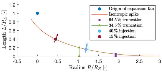
Figure 2.
Normalised nozzle contour with graphical representations for truncations, secondary injection positions and orientations, an adaptation of [21].
2.3. Realisation of the Test Specimen
Figure 3 illustrates the four types of plugs (supersonic part of the nozzle) used for the experiment. Each of the plugs differs from its numerical predecessor in a single geometric parameter. Plug 1 serves as the reference plug, exhibiting the longest truncation without secondary injection. Plug 2 shares the same length but with corresponding downstream secondary injection site. The plug analogous to the truncation length of plug 2 with an upstream injection site is labelled plug 3. Finally, plug 4 shares the injection site with plug 3, but has the shortest truncation length. Each injection site is fed symmetrically by the second gas supply line through a steel tube with an inner diameter of .
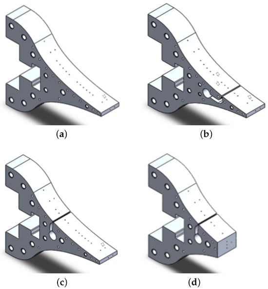
Figure 3.
Exchangeable plug specimens with their relative truncation and injection site . (a) Plug 1 ; (b) Plug 2 ; (c) Plug 3 ; (d) Plug 4 .
The plugs were manufactured with a number of pressure measurement holes, which were all aligned the plug’s median line. On the side of the plug with the secondary injection, the measurement positions were spaced with an axial distance of ≈7 mm with a doubled density near the injection sites (named suffix A). The locations of the secondary injection sites coincide with pressure measurement positions 04 and 07A.
In order to ensure comparable pressure measurements among all plugs, two measurement positions were duplicated on the opposite wall of the injection side, indicated as u. Three additional measurement positions were added at a distance of to one side wall, indicated as w. These were used to evaluate whether the wall shear layer development due to the acrylic side plates affects the pressure measurements along the median line.
At the base, each plug was equipped with two measurement positions, one in the centre and the other near the wall. The larger base of plug 4 allowed two additional pressure measurement positions along the median line with a lateral displacement. This allowed us to analyse whether the secondary injection had an influence on the symmetry of the pressure distribution at the nozzle base. All pressure measurement locations and the measurement ranges of the connected pressure sensors are summarised in Appendix A Table A1.
The test specimen was designed and manufactured as a screwed assembly. It consisted of the subsonic flow chamber, four different plugs and two acrylic side plates. The latter were used to ensure a two-dimensional flow by separating the nozzle from any lateral ambient influence. The assembled specimen is shown in Figure 4. Furthermore, in the case of plugs 2–4 with active secondary injection, the acrylic plates separated the two asymmetric nozzle flows from each other and prevented backflow around the plug due to the differential pressure.
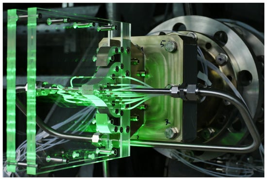
Figure 4.
Aerospike nozzle with plug 4 on the test bench.
The subsonic flow chamber serves as the mechanical interface between the specimen and the test bench. Furthermore, it realises the gas flow distribution by adapting the flow cross-section to a rectangle of , which aligns with the nozzle width . Further downstream, the flow is then separated by two symmetric channels, which continuously decrease in cross-sectional area towards the nozzle throat.
3. Results
Following the description of the test setup in the last section, the measurement results are presented here. First of all, an overview of the test sequence used for the different plugs is given. The surface pressure measurements are then analysed for the different plugs and flow states, including their dependence on secondary injection pressure. Finally, the base pressure measurements are presented and analysed with respect to their dependency on the secondary injection.
3.1. Test Sequence
For a measurement run, the maximum feeding pressures of both the primary and injection flows were set to the maximum desired value ( and , if not otherwise specified), while the control valves were used to achieve the specified pressure levels. Figure 5 shows the applied test sequences for reference nozzle plug 1 and plugs 2–4 with active injection.
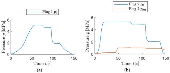
Figure 5.
Test sequences used in the presented test campaign. (a) Test sequence without SI (Plug 1). (b) Test sequence with SI (Plugs 2–4).
Both test sequences had a similar main flow total pressure profile, which began with a ramp-up transition to the highest level. After reaching the first plateau, two further steady flow conditions followed at lower pressure levels. Each of the plateaus lasted . The main flow valve was then closed and the test was completed.
In the case of active secondary injection, the first main flow plateau consists of two phases of each. The first had no active injection, but the second did. Then, after the start of the test, the injection flow control valve was fully opened and remained unchanged during the test, as did the pressure regulators. Figure 5 shows two sensor patterns that were not directly intuitive. First, during the test time between 5 and , the pressure reading for increased. This could be due to the filling of the cavity between the control valve and the injection site. The injection site, therefore, acted as a pressure measurement port with a large time constant. The second pattern was observed at about , where decreased significantly as dropped. Here, both pressures seemed to be coupled, a topic that is discussed in detail in Section 4.2.
3.2. Plug Surface Pressure
With the test sequences defined, the measurement results are presented, starting with the plug surface pressure. The pressure measurements are shown as averaged values of the stead-state phases for the main and secondary injection flows at different flow conditions.
3.2.1. Reference Nozzle—Plug 1
The pressure distribution of the reference plug 1 is shown in Figure 6 for different main flow conditions. For the under-expanded flow conditions of and , the normalised pressure ratio decreased continuously in an almost identical and ideal isentropic manner. This behaviour was due to the fact that, above the design pressure ratio (), the pressure adaptation of the nozzle flow was only realised beyond the nozzle surface and, therefore, did not affect the normalised pressure distribution on the plug surface. A deviation from this behaviour was seen at the most downstream measurement positions for the over-expanded flow condition of . Here, the normalised pressure ratio increased downstream from the nozzle position . This was due to the recompression that occurs downstream of the last expansion wave originating from the outer nozzle lip, which expanded the flow to . As the nozzle contour was designed for further expansion, the flow had turned further and created compression waves [3,4]. The compression waves then propagated to the outer shear layer, from which a second expansion fan started. The last expansion wave and the first compression line can be seen in the corresponding Schlieren images in Figure 7.
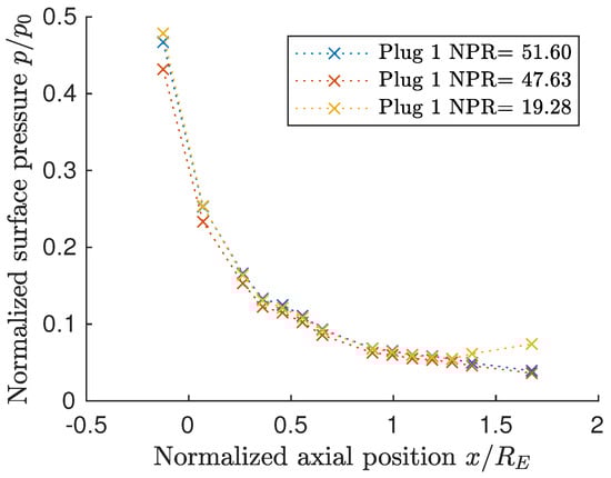
Figure 6.
Surface pressure ratio distribution of plug 1 along the axis at different main flow conditions.
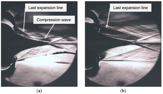
Figure 7.
Schlieren pictures of plug 1 at different main flow conditions. (a) Over-expanded flow (). (b) Under-expanded flow ().
3.2.2. Nozzles with Secondary Injection—Plugs 2–4
The surface pressure analysis with active SITVC is described for two flow conditions. The measurements of and were used here, as the second under-expanded flow condition was very similar to the latter. Figure 8a shows the measured pressure ratios for plugs 2 to 4. In the case of the over-expanded flow condition (), there was a distinct pressure increase upstream from the respective injection position for each plug. This narrow high-pressure region was found to be very similar for the identical injection positions of plugs 3 and 4. For plug 2 with the downstream injection position, the pressure rise was more extended with a gentler gradient. Downstream from the injection, a pressure drop was measured for all three plugs, where it was the highest directly at the injection site and then leveled off further downstream. For plug 3 in particular, this zone of reduced pressure appeared to be regionally confined. This confinement cannot be clearly stated for plug 4, as it was truncated at the axial position , which coincided with the approximate end of the low-pressure region. In general, this region of reduced pressure was very similar for plugs 3 and 4, whereas a different behaviour was observed for the injection downstream from plug 2. Here, a reduced pressure increase for plug 3 was observed with respect to plug 2, indicating an interaction of the compression waves with the injection flows, depending on their respective positions.
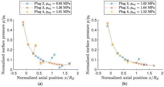
Figure 8.
Axial surface pressure ratio distribution of plugs 2–4 at different main flow conditions. (a) Over-expanded flow (). (b) Under-expanded flow ().
For the under-expanded flow condition of , the measured influence of the secondary injection on the primary flow pressure distribution was significantly less pronounced, as shown in Figure 8b. A high-pressure region in front of the upstream injection (plugs 3 and 4) could not be measured with the test specimens under these conditions. Only the downstream injection at plug 2 showed such a high-pressure region. On the other hand, the low-pressure regions downstream from the injection are clearly visible for the upstream injections (), while, for the downstream injection at , there is no significant pressure drop.
Finally, it should be noted that the measured static injection pressure diverged significantly for both flow conditions ( / )—see the legend for Figure 8. This occurred despite the fact that the pressure regulator setting and the control valve opening were not changed during the test of each plug, indicating a back-coupling of the main flow static pressure into the injection flow. This back-coupling suggested that, at least for some flow conditions, the injection flow was subsonic.
For visualisation purposes, the corresponding Schlieren images obtained during the experiments are shown in Figure 9 for plug 2 and the flow conditions discussed in Figure 8. The relevant flow characteristics of an aerospike nozzle flow caused by secondary injection are highlighted using a scheme for a sonic jet in cross-flow (see Figure 10; according to Gruber et al. [29] and Yan et al. [30]) and a Schlieren image of plug 2 at (see Figure 9a). The additional complex shock system induced in the aerospike nozzle flow was caused by the injection flow acting as an obstacle to the main flow. As a result, the supersonic main flow was deflected by an oblique shock, the separation shock, upstream from the injection position. A pair of counter-rotating recirculation zones was formed between the detached flow and the nozzle wall, creating the high-pressure zone. The separation shock joined the bow shock downstream, which originated near the injection location. The bow shock extended to the outer shear layer, buckling it, and was reflected back towards the nozzle axis. Downstream from the injection site, the flow reattached to the wall and confined the low-pressure zone formed by a third recirculation zone. In the case of the over-expanded flow in Figure 9a, a dedicated recompression shock wave due to SI could not be clearly distinguished from the compression wave originating from the reflected last expansion wave. In Figure 9b, such a dedicated recompression shock wave can be identified, which is missing on the opposite side of the nozzle flow.
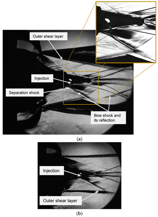
Figure 9.
Schlieren images of plug 2 with active injection at different flow conditions. (a) Over-expanded flow (). (b) Under-expanded flow ().
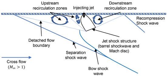
Figure 10.
Schematic of the flow phenomena of a sonic jet in cross-flow (adaptation from [17]).
Figure 9b shows the corresponding Schlieren image for plug 2 in the under-expanded flow condition. Comparing the two images, it can be seen that the formation of the flow phenomena was much more pronounced for the over-expanded main flow: the injection zone between the bow and the reattachment shock was much more bulbous and the buckling of the shear layer was more pronounced. This was due to a higher mass flow ratio of the injection flow with respect to the main flow. Furthermore, it can be observed that the central flow, downstream from the plug, was significantly asymmetric and had bent downwards, indicating a significant deflection of the thrust vector. Conversely, in the case of the under-expanded flow, the effect of the SI on the overall flow was less effective. To complete the set of Schlieren images, Figure A1 in Appendix A shows the flow states of and for plugs 3 and 4, respectively.
3.2.3. Influence of Injection Pressure on Plugs 2–4
This section presents the investigation of the influence of secondary injection pressure on the surface pressure distribution on the nozzle. This analysis has been carried out for plugs 2–4 at three different injection regulator settings between and . All data presented here are for the over-expanded flow condition of each plug at . The pressure distribution for each plug and the corresponding measured injection line pressures are shown in the following graphs.
First, Figure 11 shows the normalised surface pressure obtained for plug 2 at = 0.61–0.93 . These data show that the high-pressure region upstream and the low-pressure region downstream from the injection location were spread at least over the two adjacent measurement points. Therefore, their length was determined to be at least . The upstream high-pressure region was shorter than because position 06 was not affected by the injection. At the downstream injection, the length could not be determined precisely, as the last measurement position 10 depicted small deviations. This indicated either a very small influence of the injection or small variations in the total pressure of the main flow. For the latter, this means that a variation in the contact position of the last expansion wave and the corresponding pressure increase downstream was imminent due to the compression waves. Furthermore, as increased, the pressure profile changed from concave to linear to convex, indicating an increasing length of the high-pressure region. For example, for , the pressure signal at position 06A () seems to be almost unaffected by the injection, suggesting that the origin of the separation shock was very close to this position. Finally, it can be seen from these measurements that, as increases, the deviation of the pressure in the highand low-pressure regions caused by the injection also increases accordingly.
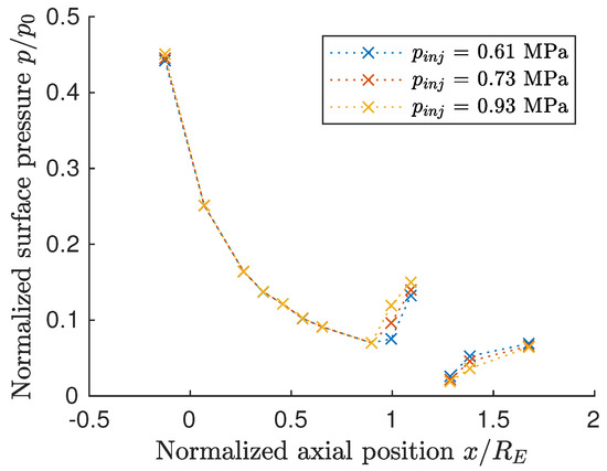
Figure 11.
Surface pressure ratio of plug 2 along the axis at different injection conditions ().
Figure 12 shows the measurements obtained for plug 3 at injection pressures = 0.91–1.36 . Firstly, it can be seen that the high-pressure region upstream from the injection is smaller than on plug 2 when compared to the distribution shown in Figure 11. The length can, therefore, be determined to be between and , as only one measurement position was affected. The length of the downstream low-pressure region is also limited, for which the data also show almost negligible deviations in the second following position 05 (). Further downstream, there were no deviations in the pressure signal, except at the very last position. This variation corresponds again to the slight deviations in the contact point between the nozzle surface and the last expansion wave. The high- and low-pressure regions differ significantly in their respective magnitudes. While the pressure increase upstream from the injection was clearly visible, the pressure decrease in the low-pressure region was almost negligible.
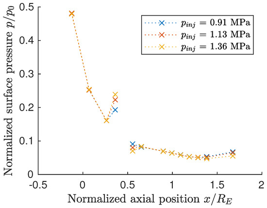
Figure 12.
Surface pressure ratio of plug 3 along the axis at different injection conditions ().
The final analysis with respect to injection pressure is shown in Figure 13 for plug 4 and = 0.68–1.01 . The general pressure signal was comparable to that of plug 3 up to the nozzle truncation. The length of the upstream high-pressure region could be estimated to be between and , as only one pressure measurement location was effected. The downstream low-pressure region, however, extended beyond position 05 , but not to position 06.
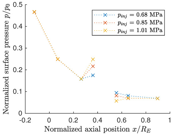
Figure 13.
Surface pressure ratio of plug 4 along the axis at different injection conditions ().
To conclude this analysis, it can be stated that the high- and low-pressure regions were directly influenced by the injection pressure. The size of these regions increased with increasing pressure, but depended even more on the injection location and, therefore, on the static pressure of the main flow. It has also been shown experimentally that higher injection pressure led to a higher pressure increase upstream and lower pressure decrease downstream from the injection location. However, in order to quantify the surface pressure distribution in more detail, a higher measurement density would be required for this test setup.
3.3. Base Pressure Measurements
The base pressure measurements are the second set of results presented here. These values are not averaged but evaluated over time during the transition between pressure levels. This allows the correlation between base pressure and nozzle pressure ratio to be analysed as a function of truncation and secondary injection.
3.3.1. Base Pressure without Secondary Injection
In the first transient phase of each test sequence, the base pressure ratio with secondary injection inactive was evaluated with respect to the . This correlation of and is shown in Figure 14 for all plugs and measurement positions over the entire captured range.
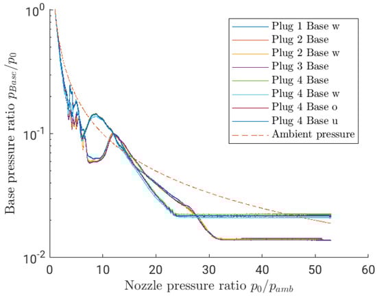
Figure 14.
Base pressure ratio over without SI.
It can be seen that the two truncation variants ( for plugs 1–3; for plug 4) show similar but different behaviour. Up to , the base pressure ratio for all plugs decreased continuously and more steeply than the ambient pressure, followed by a series of sharp oscillations up to . Furthermore, the -behaviour started to differ depending on the truncation. The base pressure ratio for plugs 1–3 (longer plugs) continued to decrease to a local minimum, followed by a local maximum near , where the base pressure locally exceeded the ambient pressure. At higher s, the base pressure ratio fell back below the ambient pressure and decreased monotonically up to , where it became constant at . This means that the base pressure depended solely on the total main flow pressure and was independent of the ambient pressure . This behaviour is widely known in the literature as ‘wake closure’. In the observed closed-wake state of plugs 1–3, the base pressure remained below the ambient pressure. Therefore, a higher would be required to achieve a net thrust gain for the base area.
For the shorter plug 4, the local maximum of the base pressure ratio occurred at , which was also above the ambient pressure ratio . The maximum was followed by a monotonous decrease, until became constant with for . At above , the base pressure exceeded the ambient pressure and, thus, caused a net thrust gain for the base area.
3.3.2. Impact of Secondary Injection on the Base Pressure
Two transients during the main flow pressure reduction (from to ) were used to evaluate the influence of the secondary injection flow on the base pressure. Figure 15 shows the base pressure ratios for the central measurements with and without injection flow for plugs 2–4. For the longer plugs 2 and 3, a minimal increase in base pressure from without secondary injection to with SI was observed. For higher above 40, this pressure increase due to SI seemed to disappear for the more upstream injection for plug 3. However, the effects near the wake transition were different. For plug 2, the measurement in the injection case closely followed the non-injection case with a small offset.
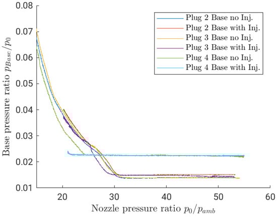
Figure 15.
Base pressure change at different s with SI.
As for plug 3, the base pressure with active injection behaved differently. On the one hand, the wake-closing transition was slightly shifted to a lower from ≈32 to ≈28. On the other hand, for below the transition phase, the base pressure was slightly below the non-injection case, except for a narrow range of intersection around .
For the shorter plug 4, there was no change in base pressure due to secondary injection observed. remained identical to the closed-wake condition for the non-injection case. However, the wake-closing transition was significantly shifted to a lower from ≈24 to ≈21 for the injection case.
In order to rule out any hysteresis effects on the wake-closing behaviour, the base pressure measurements for plug 1 (without secondary injection) are shown in Figure 16 for the same main flow transitions as the above studied plugs 2–4. It can be observed that the base pressure measurements behaved in the same way for the ramp-down of the and for the transition phase of the ramp-up. Hence, there was no significant hysteresis effect of the base pressure behaviour with respect to the gradient and direction of the progression. Consequently, the observed change in for the wake-closing transition was most likely due to the secondary injection.
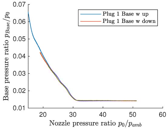
Figure 16.
Base pressure on plug 1 at different s when ramping up and down.
At this point, it can be summarised for the injection position that, for the case of upstream injection (plugs 3 and 4), active secondary injection shifts the wake-closing transition to a lower . On the other hand, for the case of downstream injection (plug 2), the secondary injection seemed to have no effect on the transition. With respect to truncation, the base pressure level showed a slight increase for the less-truncated plugs (plugs 2 and 3). However, in the case of higher truncation (plug 4), it appeared to remain unaffected by the injection flow. Consequently, the secondary injection creates opposing effects on the thrust component generated by the pressure acting on the base surface. In those cases where the base pressure is increased, the base thrust is increased. Conversely, if the wake-closing transition is shifted to lower s, the base thrust is decreased through the influence of secondary injection.
3.3.3. Flow Symmetry Analysis of Plug 4
Finally, a possible flow asymmetry due to axis-asymmetric secondary injection was investigated for plug 4. Figure 17 shows the pressure ratio for the three centreline measurements for the inactive and active injection cases. Once again, the secondary injection appeared to have no significant effect on the overall pressure level at the base in closed-wake mode. However, SI shifted the wake-closing transition to a smaller —from ≈24 to ≈21. Furthermore, active injection did not cause a significant difference between the pressure measurement closer to the injection side and the opposite side . Table 2 shows the base pressure measurements for each position averaged in the closed-wake condition of . These figures show that the overall pressure increase due to SI was greater than any asymmetry in the base pressure measurements. Therefore, only a small wake asymmetry could be observed with this setup and flow condition. The only significant deviation in the measurements can be observed up to , where the axial measurement was significantly lower than the non-axial ones ( and ). This could be attributed to the different distances between the measuring positions from the truncation edge, along with the corresponding suction effect of the detaching primary flow.
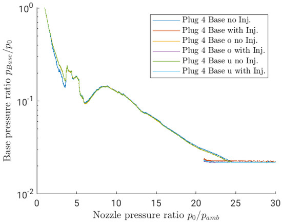
Figure 17.
Base pressure change on Plug 4 at different s due to SI.
Table 2.
Averaged base pressure ratio and change due to SI of plug 4 in closed-wake conditions.
4. Discussion
The results presented are briefly discussed and analysed in the following section. First, the influence of the acrylic side plates on the pressure measurements obtained is examined. Subsequently, a follow-up test campaign in our own laboratory is briefly described and evaluated to further analyse the reason for the variations in injection pressure and to verify the assumption of a potential subsonic injection flow.
4.1. Analysis of the Impact of the Side Plates on the Two-Dimensional Flow
An analysis to evaluate the quality of the measurements was carried out with respect to the pressure deviations in the lateral direction of the nozzle surface. For this purpose, the data obtained at the measurement positions close to the wall (index w) are compared with those of the centre line using the following normalised pressure difference: with positions # = [02;10]. The results of this assessment are shown in Figure 18 for plugs 2 and 4 over the full range during ramp-up without secondary injection and during ramp-down with SI active.

Figure 18.
Normalised difference between wall and center-line pressure of plugs 2 and 4 at different main and injection flow conditions. (a) Plug 2. (b) Plug 4.
Figure 18a shows for measurement positions 02 and 10. It can be seen that the data differed significantly depending on the position. appears to be a constant line with an average of +0.6% over the full span for inactive SI, while no significant deviation could be observed for the case with active SI. However, the noise on the signal is clearly noticeable, especially at low s. This high noise ratio is due to the high measuring range of 700 and 3500 kPa for the sensors at position 02, whereas the measuring range of the sensors at position 10 was only 100 kPa. At higher s, the noise became less pronounced due to a better signal-to-noise ratio. However, shows a significantly less noisy signal over the range with average values of +0.6% for inactive SI and +0.1% for active SI. Furthermore, the downstream measurement depicts a different behaviour. While the noise is much lower, the locally averaged value over was not constant. On the contrary, in the range of 3–26, there are significant deviations from a near-zero average, especially in the range of 20–26, where the last expansion wave interacts with the end of the plug surface (see Section 3.2.1)—these deviations reach values up to . The wavy nature of indicates that the interaction of the last expansion wave with the plug surface occurs at different s. This implies that the contact line between the last expansion wave and the surface might exhibit slight curvature, indicating a deviation from the ideal two-dimensional flow.
For comparison, Figure 18b shows these data for plug 4 at measurement position 02. It can be seen that behaves almost identically to plug 2, except for minor artefacts. The averaged values of are −0.6% with inactive injection and −0.8% with active injection.
Based on the evaluation of the pressure differences for the two positions on the spike surface, it can be concluded that, for the more upstream pressure measurement position 02, two-dimensional flow can be guaranteed for all s in the investigated range. For the downstream location 10, this is true when the last expansion wave has passed this location for s above 30. Hence, it appears that the shear layer created by the side plates had a significant influence on the shape of the expansion system in the lateral nozzle direction. Furthermore, this analysis shows a small effect of the secondary injection on the normalised pressure difference. For the upstream position 02 and both plugs, this difference seems to be slightly reduced. On the other hand, for the downstream position 10, the SI seems to increase the amplitude and slightly decrease the mean value of the wave within the range of 20–26. Though the effects are limited, an influence of the side plates on the measured pressure values cannot be completely excluded.
4.2. Injection Velocity
As mentioned in Section 3.1, changed simultaneously with the total main flow pressure during the test run, despite the fact that the pressure setting in the regulator and the control valve setting were unchanged. Therefore, a coupling of and was assumed, which would imply that the injection was at least partially subsonic rather than sonic over the entire cross-section of the injection port.
In order to verify this assumption, this test campaign was repeated in the vacuum wind tunnel test bench [14,31] at TUD using sub-scale nozzle models. These nozzles were scaled down by a factor of 5 in the throat area and by a factor of 10 in pressure to match the capabilities of the test bench. With this setup, a series of measurements were made for the two primary flow states: over-expanded () and under-expanded (). The injection pressure was varied over a wide range to capture the pressure ratios experienced in the original campaign (and beyond). Based on these measurements, the mass flow ratio is derived from the injection mass flow with active and inactive primary flow at specific injection pressures . The reason for this investigation is that, without a primary flow, the secondary injection (SI) flow is always sonic due to an injection to ambient pressure ratio of . Therefore, when , the injection mass flow depends not only on but also on the injection exit conditions implied by the primary flow, resulting in a subsonic flow.
The obtained –pressure ratio correlations are shown in Figure 19 for the different nozzle and primary flow conditions. In addition, the –pressure ratio correlations for the flow conditions investigated in Section 3 are marked. In general, it can be seen from this figure that there are three distinct areas in the plots. At very low , the increases linearly with the pressure ratio. Above a certain pressure ratio, which correlates with the injection position (plug 2: , plugs 3 and 4: ), the becomes unity. There is a curved transition zone between these two linear correlations.
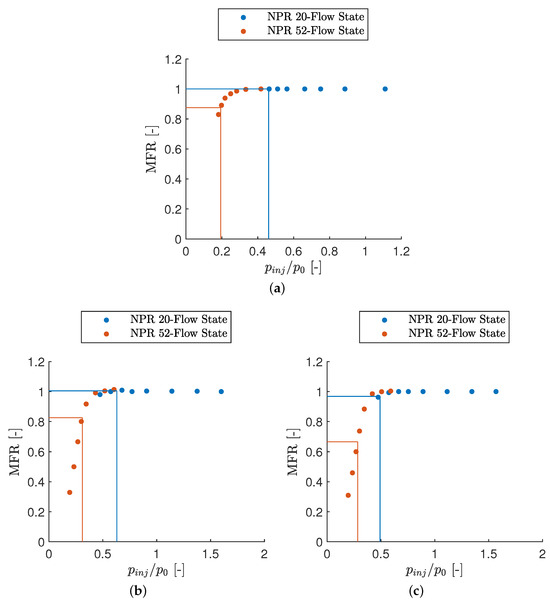
Figure 19.
Mass flow ratio–injection pressure ratio correlation obtained in the vacuum wind tunnel test campaign, with visualisation of the original test conditions. (a) Plug 2 . (b) Plug 3 . (c) Plug 4 .
It is clear from Figure 19 that, in the under-expanded primary flow condition at , the remained below 1 for all three plugs and the injection was subsonic. The situation is different for the under-expanded primary flow condition at : for plug 2 with downstream injection, is high enough to ensure sonic injection. The pressure ratio for plug 3 is very close to the critical value required for sonic injection and appears to be just above this threshold. However, the injection flow of plug 4 is below the threshold and in the transitional range close to full sonic injection.
It can, therefore, be concluded that sub- or transsonic injection has been achieved in most of the experiments conducted. Sonic injection was only achieved in a few experimental phases, particularly in the over-expanded primary flow state. It is, therefore, critical to achieve a pressure ratio above the threshold to ensure sonic injection. In the presented test campaign, it is assumed that the relatively small diameter of the metal hose in the injection line caused a high pressure loss, which prevented the required pressure ratio for sonic injection from being achieved across all experimental phases.
However, these results are not only relevant in terms of knowledge gain and CFD validation per se, but are also essential for engineering such SITVC systems for thrust-vectoring aerospike nozzles. The engineer can either ensure sonic injection by maintaining a ratio above the threshold or can adapt the controller for the more complex interactions with the main flow when subsonic injection conditions occur. The latter is particularly applicable when the SITVC is not simply switched on and off, like in a fast-opening and -closing solenoid valve, but rather with a continuously adjustable flow control valve.
5. Conclusions
A cold-gas test campaign with different linear aerospike nozzles and thrust vector control by secondary injection was carried out at the DLR test bench P6.2 in Lampoldshausen. The different nozzles were realised by interchangeable plugs—the supersonic part of the aerospike nozzle—which allowed the investigation of two truncations and two injection positions each. The objective of measuring the surface pressure along the nozzle wall and the nozzle base under different main flow conditions (over- and under-expanded) with a secondary injection was achieved, and the following results were obtained:
- It can be seen that there is a high-pressure zone upstream and a low-pressure zone downstream from the injection position, which are in good agreement with previous publications based on CFD analysis.
- Based on measurements at different injection pressures, it can be concluded that, as the injection pressure increases, the pressure deviation of the high- and low-pressure zones from the nominal flow without injection increases. The measurement results also indicate that the dimensions of both pressure zones increase as the injection pressure increases;
- It was observed that truncation and injection position have an interdependent influence on base pressure and wake-closure behaviour. A slight increase in base pressure due to secondary injection was observed for the plugs with less truncation , whereas no change in base pressure was observed for the plug with higher truncation . On the other hand, the upstream injection position showed a significant influence on the wake-closure behaviour for both truncation lengths, reducing the critical nozzle pressure ratio at which the wake closure transition occurred. No such influence was observed for the downstream injection .
- The critical pressure ratio between injection and primary flow was investigated in a follow-up campaign to ensure sonic injection. This critical pressure ratio was found to be dependent on the injection position and showed that the injection flow during the main test campaign was in the transsonic regime. In addition, subsonic injection was characterised by a reduced mass flow, injection velocity and, consequently, thrust in comparison to an equivalent nozzle with sonic flow. It is, therefore, uncertain to what extent these losses can be compensated with the aerodynamic side-force gain from the interaction of the main and injection flows, requiring further investigation.
In conclusion, the results of the presented test campaign provide a first insight into the surface pressure distribution on aerospike nozzles in combination with secondary injection thrust vector control. The results show that truncation and injection cause interdependent variations on the ideal isentropic expansion of the aerospike nozzle, which deserve further in-depth analysis. Finally, they can be used as a validation approach for numerical simulations of comparable flow scenarios.
Author Contributions
Conceptualisation, J.S.-K., M.P., R.H.S. and C.B.; methodology, J.S.-K. and M.P.; software, D.S. and S.G.; validation, J.S.-K., M.P., R.H.S., D.S. and S.G.; formal analysis, J.S.-K.; investigation, J.S.-K., M.P., R.H.S., D.S., S.G. and C.B.; resources, R.H.S. and M.T.; data curation, R.H.S., D.S. and S.G.; writing—original draft preparation, J.S.-K. and M.P.; writing—review and editing, all authors; visualisation, J.S.-K. and M.P.; supervision, M.T.; project administration, J.S.-K. and M.P.; funding acquisition, J.S.-K., M.P. and C.B. All authors have read and agreed to the published version of the manuscript.
Funding
This research was funded by the SAB (Sächsische Aufbaubank—Saxonian Development Bank) and the SMWK (Sächsisches Ministerium für Wissenschaft und Kunst—Saxonian Ministry for Science and Arts) (100323652).
Institutional Review Board Statement
Not applicable.
Informed Consent Statement
Not applicable.
Data Availability Statement
The data sets generated during and/or analysed during the current study are available from the corresponding author on reasonable request.
Acknowledgments
We appreciate the assistance and support by Dietmar Maier, cold-gas test bench P6.2 in Lampoldshausen, who always ensured a smooth test run. Furthermore, we are very grateful to Adheena Gana Joseph for language proofreading. At last, we would like to express our gratitude to our student Jonathan Bölk for his support in the data evaluation.
Conflicts of Interest
The authors declare no conflicts of interest. The funders had no role in the design of the study; in the collection, analyses, or interpretation of data; in the writing of the manuscript or in the decision to publish the results.
Abbreviations
The following abbreviations are used in this manuscript:
| CFD | Computational Fluid Dynamics |
| DLR | German Aerospace Center |
| GN2 | Gaseous Nitrogen |
| LF | Low Frequency |
| SI | Secondary Injection |
| TVC | Thrust Vector Control |
Appendix A

Figure A1.
Schlieren pictures of Plugs 3 and 4 with active injection at different main flow conditions. (a) Plug 3—Over-expanded flow (); (b) Plug 3—Under-expanded flow (); (c) Plug 4—Over-expanded flow (); (d) Plug 4—Under-expanded flow ().
Figure A1.
Schlieren pictures of Plugs 3 and 4 with active injection at different main flow conditions. (a) Plug 3—Over-expanded flow (); (b) Plug 3—Under-expanded flow (); (c) Plug 4—Over-expanded flow (); (d) Plug 4—Under-expanded flow ().

Table A1.
Measuring position locations on the plugs and sensor range [21].
Table A1.
Measuring position locations on the plugs and sensor range [21].
| Position | Axial Position [mm] | Sensor Range [kPa] | |
|---|---|---|---|
| Plugs 1–4 | 01 | −4.5 | 0–3500 |
| 02 (u, w, uw) | 2.5 | 0–3500 and 0–700 | |
| 03 | 9.5 | 0–700 | |
| 03A | 13.0 | 0–700 | |
| 04 | 16.5 | 0–700 | |
| 04A | 20.0 | 0–700 | |
| 05 (u) | 23.5 | 0–700 | |
| 06 | 32.3 | 0–350 | |
| Plugs 1–3 | 06A | 35.8 | 0–700 or 0–350 |
| 07 | 39.3 | 0–350 | |
| 07A | 42.8 | 0–350 | |
| 08 | 46.3 | 0–350 | |
| 08A | 49.8 | 0–50 | |
| 10 (w) | 60.3 | 0–100 | |
| Base (w) | 69.1 | 0–100 | |
| Plug 4 | Base (w) | 36.9 | 0–100 |
| (lateral position 0.0) | |||
| Base (o, u) | 36.9 | 0–100 | |
| (lateral position ) | |||
| Plugs 2–4 | Inj | – | 0–3500 |
Name affixes: o: additional position on injection side; u: additional position on opposite side; w: additional position near the wall; uw: additional combination of u and w.
References
- Fick, M.; Schmucker, R.H. Performance aspects of plug cluster nozzles. J. Spacecr. Rocket. 1996, 33, 507–512. [Google Scholar] [CrossRef]
- Rommel, T.; Hagemann, G.; Schley, C.A.; Krulle, G.; Manski, D. Plug Nozzle Flowfield Analysis. J. Propuls. Power 1997, 13, 629–634. [Google Scholar] [CrossRef]
- Hagemann, G.; Immich, H.; Nguyen, T.V.; Dumnov, G.E. Advanced Rocket Nozzles. J. Propuls. Power 1998, 14, 620–634. [Google Scholar] [CrossRef]
- Nasuti, F.; Onofri, M. Methodology to Solve Flowfields of Plug Nozzles for Future Launchers. J. Propuls. Power 1998, 14, 318–326. [Google Scholar] [CrossRef]
- Ito, T.; Fujii, K.; Hayashi, A.K. Computations of Axisymmetric Plug-Nozzle Flowfields: Flow Structures and Thrust Performance. J. Propuls. Power 2002, 18, 254–260. [Google Scholar] [CrossRef]
- Eilers, S.; Matthew, W.; Whitmore, S. Analytical and Experimental Evaluation of Aerodynamic Thrust Vectoring on an Aerospike Nozzle. In Proceedings of the 46th AIAA/ASME/SAE/ASEE Joint Propulsion Conference and Exhibit, American Institute of Aeronautics and Astronautics, Nashville, TN, USA, 25–28 July 2010. [Google Scholar] [CrossRef]
- Besnard, E.; Garvey, J. Development and Flight-Testing of Liquid Propellant Aerospike Engines. In Proceedings of the 40th AIAA/ASME/SAE/ASEE Joint Propulsion Conference and Exhibit, American Institute of Aeronautics and Astronautics, Fort Lauderdale, FL, USA, 11–14 July 2004. [Google Scholar] [CrossRef]
- Bui, T.; Murray, J.; Rogers, C.; Bartel, S.; Cesaroni, A.; Dennett, M. Flight Research of an Aerospike Nozzle Using High Power Solid Rockets. In Proceedings of the 41st AIAA/ASME/SAE/ASEE Joint Propulsion Conference and Exhibit. American Institute of Aeronautics and Astronautics, Tucson, AZ, USA, 10–13 July 2005. [Google Scholar] [CrossRef]
- Fadigati, L.; Rossi, F.; Souhair, N.; Ravaglioli, V.; Ponti, F. Development and simulation of a 3D printed liquid oxygen/liquid natural gas aerospike. Acta Astronaut. 2024, 216, 105–119. [Google Scholar] [CrossRef]
- Bach, C.; Schöngarth, S.; Bust, B.; Propst, M.; Sieder-Katzmann, J.; Tajmar, M. How to steer an aerospike. In Proceedings of the 69th International Astronautical Congress, Bremen, Germany, 1–5 October 2018. Number IAC-18-C4.3.15. [Google Scholar]
- Silver, R. Advanced Aerodynamic Spike Configurations—Hot-Firing Investigations; Final Report AFRPL-TR-67-246-Vol II AD-384 856; Rocketdyne: Los Angeles, CA, USA, 1967. [Google Scholar]
- Eilers, S.D.; Wilson, M.D.; Whitmore, S.A.; Peterson, Z.W. Side-Force Amplification on an Aerodynamically Thrust-Vectored Aerospike Nozzle. J. Propuls. Power 2012, 28, 811–819. [Google Scholar] [CrossRef]
- Eilers, S.D.; Wilson, M.D.; Whitmore, S.A. Design of a Small Scale Aerospike Nozzle and Associated Testing Infrastructure for Experimental Evaluation of Aerodynamic Thrust Vectoring. In Proceedings of the Utah Space Grant Consortium—Session 2, Logan, UT, USA, 5 October 2010; Available online: https://digitalcommons.usu.edu/spacegrant/2010/Session2/5/ (accessed on 28 September 2023).
- Sieder-Katzmann, J.; Propst, M.; Tajmar, M.; Bach, C. Investigation of Aerodynamic Thrust-Vector Control for Aerospike Nozzles in Cold-Gas Experiments. In Proceedings of the Space Propulsion 2020 + 1, Virtual, 17–19 March 2021. number SPC2020_406. [Google Scholar]
- Spaid, F.W.; Zukowski, E.E. A study of the interaction of gaseous jets from transverse slots with supersonic external flows. AIAA J. 1968, 6, 205–212. [Google Scholar] [CrossRef]
- Zukowski, E.E.; Spaid, F.W. Secondary injection of gases into a supersonic flow. AIAA J. 1964, 2, 1689–1696. [Google Scholar] [CrossRef]
- Propst, M.; Liebmann, V.; Sieder-Katzmann, J.; Bach, C.; Tajmar, M. Maximizing Side Force Generation in Aerospike Nozzles for Attitude and Trajectory Control. In Proceedings of the 69th International Astronautical Congress, Bremen, Germany, 1–5 October 2018. Number IAC-18.C4.10.4.x47139. [Google Scholar]
- Ferlauto, M.; Ferrero, A.; Marsicovetere, M.; Marsilio, R. Differential Throttling and Fluidic Thrust Vectoring in a Linear Aerospike. Int. J. Turbomach. Propuls. Power 2021, 6, 8. [Google Scholar] [CrossRef]
- Sieder, J.; Propst, M.; Bach, C.; Tajmar, M. Shallow water experiments to verify a numerical analysis on an aerodynamically thrust-vectored aerospike nozzle. Prog. Propuls. Phys. 2019, 11, 529–542. [Google Scholar] [CrossRef]
- Propst, M.; Rümmler, L.; General, S.; Liebmann, V.; Sieder-Katzmann, J.; Bach, C.; Tajmar, M. Flow Visualisation and Surface Measurements of Shallow Water Experiments Exemplary for Aerospike Nozzles with Secondary Injection. In Proceedings of the Space Propulsion Conference, Sevilla, Spain, 14–18 May 2018. Number Paper SP2018_466. [Google Scholar]
- Sieder-Katzmann, J.; Propst, M.; Stark, R.H.; Schneider, D.; General, S.; Tajmar, M.; Bach, C. ACTIVE—Experimental Setup and First Results of Cold Gas Measurments for Linear Aerospike Nozzles with Secondary Fluid Injection for Thrust Vectoring. In Proceedings of the 8th European Conference on Aeronautics and Aerospace Sciences (EUCASS), Madrid, Spain, 1–4 July 2019. number 8. [Google Scholar] [CrossRef]
- Sieder-Katzmann, J.; Propst, M.; Stark, R.; Schneider, D.; General, S.; Tajmar, M.; Bach, C. ACTiVE—Experimental investigation of the pressure distribution of linear aerospike nozzles with aerodynamic thrust vectoring. In Proceedings of the Aerospace Europe Conference 2023—10th EUCASS—9th CEAS, Lausanne, Switzerland, 9–13 July 2023. [Google Scholar] [CrossRef]
- Börger, G.G. Optimierung von Windkanaldüsen für den Unterschallbereich. Ph.D. Thesis, Technical University Brunswick, Braunschweig, Germany, 1973. [Google Scholar]
- Börger, G.G. The Optimization of Wind-Tunnel Contractions for the Subsonic Range. Ph.D. Thesis, Technical University Brunswick, Braunschweig, Germany, 1976. [Google Scholar]
- Frey, M.; Stark, R.; Cieaki, H.; Quessard, F.; Kwan, W. Subscale nozzle testing at the P6.2 test stand. In Proceedings of the 36th AIAA/ASME/SAE/ASEE Joint Propulsion Conference and Exhibit, American Institute of Aeronautics and Astronautics, Las Vegas, NV, USA, 24–28 July 2000. [Google Scholar] [CrossRef]
- Kronmüller, H.; Schäfer, K.; Zimmermann, H.; Stark, R. Cold Gas Subscale Test Facility P6.2 at DLR Lampoldshausen. In Proceedings of the 6th International Symposium on Propulsion for Space Transportation of the XXI Century, Palais des Congress, Versailles, France, 14–17 May 2002; pp. 1–8. [Google Scholar]
- Schäfer, K.; Böhm, C.; Kronmüller, H.; Stark, R.; Zimmermann, H. P6.2 Cold Gas Test Facility For Simulation of Flight Conditions—Current Activities. In Proceedings of the EUCASS 2005, Moscow, Russia, 4–7 July 2005; pp. 1–7. [Google Scholar]
- Lee, C.C. Technical Note—Fortran Programs for Plug Nozzle Design. Technical report. 1963. Available online: https://archive.org/details/nasa_techdoc_19630012259/page/n35/mode/2up (accessed on 24 September 2010).
- Gruber, M.R.; Nejad, A.S.; Chen, T.H.; Dutton, J.C. Compressibility effects in supersonic transverse injection flowfields. Phys. Fluids 1997, 9, 1448–1461. [Google Scholar] [CrossRef]
- Yan, L.; Huang, W.; Li, H.; Zhang, T.t. Numerical investigation and optimization on mixing enhancement factors in supersonic jet-to-crossflow flow fields. Acta Astronaut. 2016, 127, 321–325. [Google Scholar] [CrossRef]
- Sieder-Katzmann, J.; Propst, M.; Tajmar, M.; Bach, C. Cold Gas Experiments on Linear Thrust-Vectored Aerospike Nozzles through Secondary Injection. In Proceedings of the 70th International Astronautical Congress (IAC), Washington, DC, USA, 21–25 October 2019. number IAC-19-C4.10.8.x53736. [Google Scholar]


Disclaimer/Publisher’s Note: The statements, opinions and data contained in all publications are solely those of the individual author(s) and contributor(s) and not of MDPI and/or the editor(s). MDPI and/or the editor(s) disclaim responsibility for any injury to people or property resulting from any ideas, methods, instructions or products referred to in the content. |
© 2024 by the authors. Licensee MDPI, Basel, Switzerland. This article is an open access article distributed under the terms and conditions of the Creative Commons Attribution (CC BY) license (https://creativecommons.org/licenses/by/4.0/).