Abstract
Due to the strong nonlinearity in the reentry trajectory planning problem for reusable launch vehicles (RLVs), the scale of the problem after high-precision discretization can become significantly large, and the non-convex path constraints are prone to exceed limits. Meanwhile, the objective function oscillation phenomenon may occur due to successive convexification, which results in poor convergence. To address these issues, a novel sequential convex programming (SCP) method utilizing modified hp-adaptive mesh refinement and variable quadratic penalty is proposed in this paper. Firstly, a local mesh refinement algorithm based on constraint violation is proposed. Additional mesh intervals and mesh points are added in the vicinity of the constraint violation points, which improves the satisfaction of non-convex path constraints. Secondly, a sliding window-based mesh reduction algorithm is designed and introduced into the hp-adaptive pseudospectral (PS) method. Unnecessary mesh intervals are merged to reduce the scale of the problem. Thirdly, a variable quadratic penalty-based SCP method is proposed. The quadratic penalty term related to the iteration direction and the weight coefficient updating strategy is designed to eliminate the oscillation. Numerical simulation results show that the proposed method can strictly satisfy path constraints while the computational efficiency and convergence of SCP are improved.
1. Introduction
Reentry trajectory planning is one of the key issues faced by RLVs in achieving a soft landing. How to reduce the time consumption of high-precision trajectory generation and improve algorithm convergence is a hot research topic in this field. The reentry trajectory planning problems can generally be solved based on profile iteration [1,2], analytical solution [3], or numerical optimization methods [4,5,6,7,8,9,10,11,12]. The profile iteration method parameterizes the trajectory profile, and once the key parameters of the profile are determined by iteration, a trajectory that satisfies various constraints is obtained. However, the trajectory which is obtained by the profile iteration method is mostly not the optimal solution. The numerical optimization methods transform trajectory planning problems into optimization problems to solve and can be divided into two categories: indirect methods [4] and direct methods. The indirect method transforms the trajectory planning problem into an optimal control problem, and the problem is solved based on Pontryagin’s maximum principle, ensuring the optimality of the trajectory solution. However, it is difficult to handle complex models and multi-constraints of reentry trajectory planning problems and is sensitive to the initial value. The direct methods, including the PS method and convex programming method, discretize the trajectory and solve the corresponding non-linear parametric programming problem. The direct methods can ensure optimality and efficiency simultaneously [5,6]. Among these methods, convex optimization methods have become a promising approach for complex trajectory planning because of their computational efficiency [7,8,9,10,11,12]. The current research in convex optimization focuses on handling complex constraints [7,8,9], adapting discrete mesh [10], and improving computational efficiency [11,12], etc. However, few studies have considered that unreasonable discrete mesh may cause the violation of path constraints. Meanwhile, the scale of the problem after convexification and discretization is very large, which makes it difficult to ensure the convergence of convex optimization, and the computational efficiency and precision need to be balanced. To address these issues, the discretization and the sequential iteration process of convex optimization are further studied in this paper.
Convex optimization methods have excellent theoretical properties; that is, the global optimal solution of convex optimization problems can be obtained in polynomial time. However, trajectory optimization problems are mostly non-convex, so lossless convexification was proposed [13,14]. In lossless convexification, the non-convex terms are substituted for convex ones, and the constraints are relaxed, so the original non-convex problem is completely transformed into a convex optimization problem. It can be proved that the solution is equivalent to the optimal solution of the original problem. However, lossless convexification cannot handle more general non-convex constraints, such as dynamic constraints containing aerodynamic effects and strong nonlinear path constraints, so successive convexification was further introduced [15,16]. A series of iterations are performed, and convexification is applied in each iteration to gradually approach the solution of the original problem. The above process is abbreviated as the SCP algorithm. As the convex subproblem in the sequential iteration is only an approximation of the original problem, it is hard to guarantee the precision of the solution, especially for the reentry trajectory optimization problem with strong aerodynamic effects. Meanwhile, how to improve the convergence of the sequential iteration remains a challenging issue [17]. Therefore, relevant scholars have conducted research from two aspects, namely, the discretization methods and the improvement of the SCP algorithm.
Discretization is a key factor that affects trajectory solution precision and solving time consumption. The high-precision discretization methods can be mainly divided into three categories. The first type is the local method, which refines the mesh only in a certain part of the entire trajectory by adjusting the distribution and the number of mesh points, such as the multi-resolution techniques [18]. The number of mesh intervals and points is updated based on evaluation metrics such as interpolation midpoint error [19] and state variable smoothness [20]. The adaptive mesh refinement can also be combined with the sequential convex optimization, and the computational efficiency is improved [21]. The second type is the global method, including the PS methods, etc. [22]. In the global method, the state variables and control variables are discretized simultaneously, and the entire trajectory is fitted by interpolation polynomials, which can significantly reduce the number of mesh points without loss of discrete precision. The solving efficiency and stability are further improved through Birkhoff preprocessing [23,24]. The third type is the combination of local and global methods, such as the hp-adaptive PS method [25]. By using polynomials such as Legendre–Gauss–Radau and Hermite–Simpson in each mesh interval, the precision has been further improved. The number of mesh intervals and the order of interpolation polynomials within each interval are adaptively adjusted according to the degree of local nonlinearity [26]. Further, the SCP algorithm is utilized to solve the nonlinear programming problem under the hp Radau-PS discretization form, and the solving efficiency is improved [27,28]. However, for complex problems such as reentry trajectory optimization, how to balance the solving efficiency and accuracy remains a challenge.
To improve the convergence, the solving flow of the SCP algorithm has been modified. As the SCP algorithm is an iterative process, adaptive adjustments to the step size of each iteration [29,30,31,32,33] or trust region (maximum allowable value of step size) [34,35,36,37,38] can achieve better convergence. A line search method based on sufficient descent conditions is proposed for the reentry trajectory optimization [29]. Through the line search, a better step size can be calculated to improve the convergence. A one-dimensional line search strategy is also adopted to solve the trajectory planning problem of unmanned aerial vehicles [30]. However, the above methods are infeasible when the directional derivative of the index function is greater than 0. To achieve a greater degree of decrease in the index function during each iteration, the Goldstein condition is used as the stopping criterion for the line search [31,32]. An error feedback index and a line search filter are designed, which enhances the feasibility and precision of the iteration process by constraining the convex error range [33]. The size of the trust region radius is also one of the main factors affecting convergence. When a fixed trust region is used, the solution may be updated with the maximum step size, and the objective function may oscillate near the optimal solution, resulting in poor convergence [34]. This characteristic is called the oscillation phenomenon or solution chattering [35]. It is theoretically proved that the oscillation phenomenon is an inherent property of trust region-based SCP methods. To overcome the oscillation phenomenon, a hybrid switching SCP algorithm based on oscillation occurrence condition judgment is proposed [36]. The trust region is processed as a soft constraint when oscillation occurs, which improves the convergence of sequential convex programming algorithms. Further, the SCP methods based on high-order trust regions [37] and hybrid-order trust regions [38] have been proposed successively. In Refs. [37,38], the trust region radius terms with different orders are added into the objective function, which can improve the convergence and optimality of the SCP method.
Although the aforementioned works have achieved great progress in high-precision discretization and the improvement of the SCP algorithm, there are still several issues for reentry trajectory optimization that need to be further considered.
- (1)
- The function of the reentry path constraint is nonlinear; the maximum point may be located between two adjacent mesh points. When the local mesh points are few, the fitting precision of the nonlinear function is insufficient. This means that even if the path constraint is satisfied at all mesh points, it will still exceed the limits within a certain time interval in the vicinity of the maximum point. However, most of the existing methods for reentry trajectory optimization lack consideration for such situations.
- (2)
- After achieving the desired mesh precision, the convergent fixed mesh is commonly used in the subsequent optimization process. However, for the reentry problems with strong nonlinear aerodynamic effects, the number of mesh intervals and points after mesh convergence may be very large, which results in a decrease in computational efficiency and even infeasibility. Therefore, it is necessary to perform mesh reduction to improve optimization efficiency.
- (3)
- Many studies add fixed penalty functions into the objective function to improve convergence. Our numerical simulation shows that the weight coefficient of the additional penalty item has a significant impact on the SCP solution process. An excessive coefficient value can lead to premature convergence and a decrease in optimality, while a small coefficient value can cause a slow convergence rate and even an oscillation phenomenon. Hence, how to select coefficient values reasonably needs to be further studied.
Based on the above analysis, an SCP method utilizing modified hp-adaptive mesh refinement and variable quadratic penalty is proposed in this paper. The main contributions are summarized as follows:
- (1)
- Under the hp-adaptive PS discretization framework, a local mesh refinement algorithm is designed. The violation points of path constraints are accurately detected, and additional mesh points are added in the vicinity of these violation points. With the consideration of path constraint extreme points in mesh refinement, the satisfaction of the non-convex constraints is improved;
- (2)
- A mesh reduction method based on a sliding window algorithm is proposed. The state error within each mesh interval is evaluated explicitly and rapidly via the Birkhoff polynomial. The mesh intervals within the sliding window are judged as to whether they can be merged according to the solution error. Thus, the scale of the discrete problem is reduced without loss of precision;
- (3)
- A variable quadratic penalty-based SCP method is proposed. When the objective function oscillation phenomenon occurs, the quadratic penalty is introduced into the original objective function, and the penalty coefficient is adaptively adjusted according to the iteration histories. Numerical simulation reveals that the proposed method can overcome the oscillation and improve convergence.
The organization of this paper is as follows. Section 2 introduces the trajectory optimization model for RLV and a multi-stage SCP framework. Section 3 presents a modified hp-adaptive mesh refinement method, which provides a lightweight high-precision discrete programming model for the SCP algorithm. In Section 4, the convex optimization model under the hp-adaptive PS discretization format is constructed, and a variable quadratic penalty-based SCP method is proposed. Simulations are given in Section 5, and the conclusion is provided in Section 6.
2. Problem Formulation and Multi-Stage SCP Framework
2.1. Problem Formulation
- RLV reentry dynamics
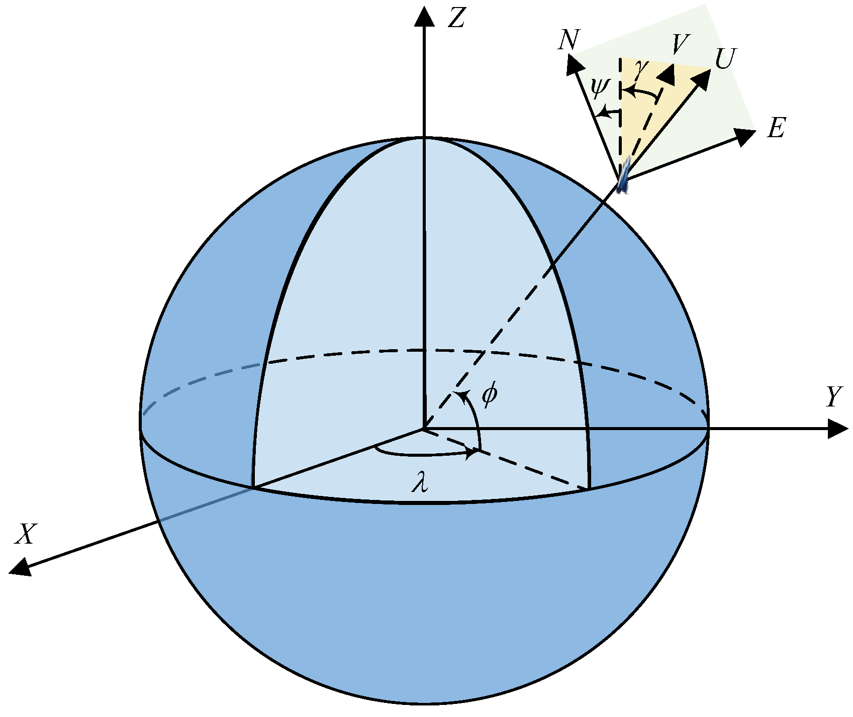
In order to increase the feasible range of trajectory solution and ensure the smoothness of flight, the change rate of angle of attack and bank angle are selected as new control variables. The original control variables and are introduced into the state variables. Hence, based on the three-dimensional equations of motion in Ref. [39], the reentry dynamics model for RLVs with expanded state variables can be given by Equation (1). Figure 1 shows the definition of state variables.
where is the geocentric distance which denotes the distance from the Earth’s center to the vehicle, is the velocity of the vehicle, and denote the longitude and the latitude, is the flight path angle which denotes the angle between the velocity vector and the local horizontal, is the heading angle which denotes the angle between the north direction and the projection of the velocity vector onto the local horizontal plane, is the angle of attack, which denotes the angle between the velocity vector and the vehicle body axis, is the bank angle which denotes the roll angle of the vehicle about the velocity vector, is the new control vector. are the function terms related to Earth’s rotation, which is given in Ref. [39].
where is the Earth’s rotation velocity. and are the dimensionless forms of lift force and drag force, which can be expressed as
where and are the reference area and the mass of the RLV; and are the coefficients of lift force and drag force, which are related to and . The atmospheric density is given by
where is the standard atmospheric density, is the current height, and is a constant value.

Figure 1.
Definition of the state variables.
- 2.
- Objective function
To ensure that RLV reaches the target point as quickly as possible while the control variable changes smoothly, the objective function which consists of two parts is considered. The first part of minimizes the total flight time. Meanwhile, the second part is an integral type indicator which minimizes the change rate of the control profile.
where and are the initial and terminal times, respectively, is the control variable, i.e., and at , and are constant coefficients, which are given manually. The integral term can reduce the oscillation of the control variable and improve the smoothness of the control profile. By minimizing , an optimal trajectory that balances arrival speed and control smoothness is obtained.
- 3.
- Control variable constraints
Unlike traditional fixed angle-of-attack profile schemes, the direct control variables of the trajectory optimization model in this paper are and . The constraints related to the control variables can be described as
where ; ; and denote the lower bound for and ; and denote the upper bound for and .
- 4.
- Path constraints
Typical path constraints, including dynamic pressure constraint , overload constraint , and heating rate constraint are considered in this paper, which can be given by
where is a constant related to the external structure of the RLV.
- 5.
- Boundary constraints
The initial conditions for the trajectory optimization problem in this paper can be described as
where denotes the initial condition of RLV. The terminal state constraints can be described as
where the superscript “” represents the expected terminal state.
In summary, the reentry trajectory optimization problem can be described as a typical optimal control problem P0, which is to find optimal control that satisfies the above constraints. The mathematical form of P0 is given by
where is the right-hand function term of the dynamic equation; is the unified expression of path constraints; is the limit value of the i-th path constraint.
2.2. Solving Framework Based on SCP Method
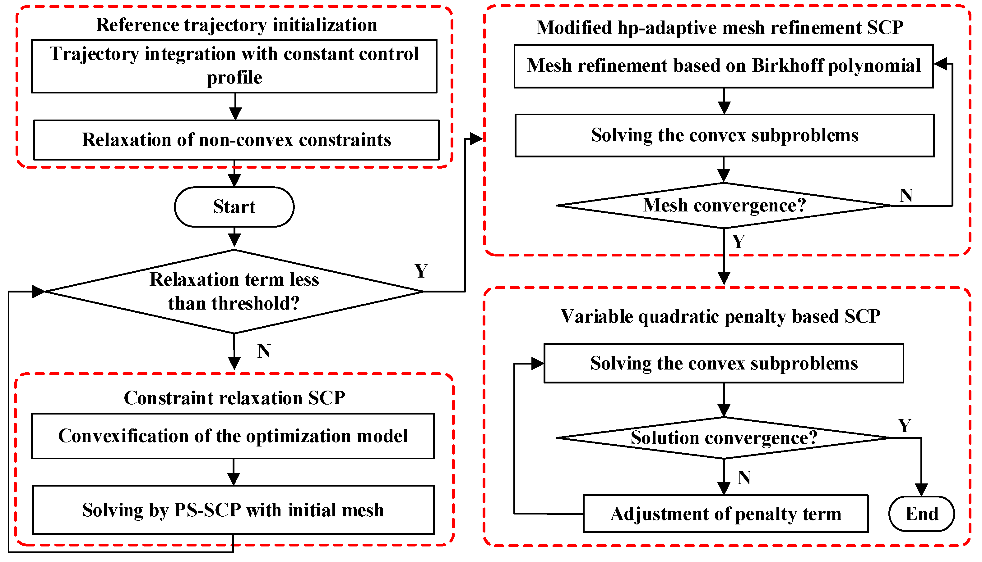
As shown in Figure 2, a multi-stage SCP framework which consists of four stages is proposed in this paper to improve the solution precision and convergence. In the first stage, a reference trajectory is generated, and the constraint relaxation optimization model is constructed for the subsequent SCP-solving process. In the second stage, the relaxed problem is solved by SCP with initial mesh, which is fixed during the iteration. When the relaxation term is small enough, Stage 3 starts. In Stage 3, the mesh is refined in each iteration under the modified hp-adaptive strategy, which increases the discrete precision gradually until the mesh converges. In Stage 4, the problem is solved with the converged mesh obtained from Stage 3, and the variable quadratic penalty is introduced into the SCP algorithm. The iteration of the SCP algorithm continues until the solution converges.
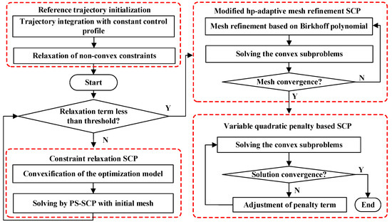
Figure 2.
The framework of the proposed multi-stage SCP method.
The specific explanations of the four stages are as follows:
Stage 1: Reference trajectory initialization. The initial solution is obtained by trajectory integration with a constant control profile. Then, the virtual control and are introduced to relax the strong non-convex terms to avoid infeasible situations caused by the rough initial solution. The form of problem P1 after relaxation is given by
where and are constant values; and represent the relaxation terms of dynamic constraints and path constraints, respectively. As the iteration progresses, the value of and are set to 0, which can ensure the satisfaction of the original constraints.
Stage 2: Constraint relaxation SCP. In this stage, the constraint relaxation trajectory optimization model is transformed into a convex optimization subproblem. Then, the convex problem is solved via the basic SCP method under fixed discrete mesh. The specific process of convexification and PS discretization will be given in subsequent chapters. When Equation (12) is established, move on to the next stage.
where is a preset threshold.
Stage 3: Hp-adaptive mesh refinement SCP. To improve the discretization precision, the distribution of mesh points is adaptively adjusted in this stage. The number of mesh intervals and points is increased or reduced based on solution error evaluation. When the error meets the precision requirements, and the number of mesh intervals and points remains the same, the mesh is considered to converge.
Stage 4: Variable quadratic penalty-based SCP. The converged mesh obtained from Stage 3 is used in this stage. The variable quadratic penalty term is introduced to improve the convergence of the SCP algorithm. Assuming the trajectory result obtained from the k-th iteration is , when Equation (13) is met
the algorithm converges and is the solution to the original problem.
3. Modified hp-Adaptive Mesh Refinement Method Based on PS Discretization
3.1. Hp Pseudospectral Discretization
To improve the precision of the trajectory solution, this paper combines the hp-adaptive strategy with the PS method. The h and p denote the number of mesh intervals and the number of mesh points within a mesh interval, respectively. The PS method is a type of method that uses global interpolation polynomials to approximate state and control variables at a set of mesh points. When the mesh points are the roots of a specific polynomial (e.g., Chebyshev or Legendre polynomials), the precision of the approximation is significantly enhanced. During the solution process, h and p are adaptively adjusted simultaneously to further improve precision in this paper.
To achieve hp adaptation, the discretization process with fixed hp is first introduced. When the total number of mesh intervals F, the number of mesh points Ni in each interval and time domain range of the trajectory are given, the distribution of mesh points, as well as the state vectors and control vectors , and time-domain transformation coefficient within each interval are obtained. The discretized dynamic constraints are obtained through the PS method. Next, the vectors within each interval are organized into a unified vector, respectively, and all continuous constraints are converted into discrete constraints about this unified vector. Finally, the discretized problem P2 is obtained. The pseudocode of the above process is given as Algorithm 1.
| Algorithm 1. Hp pseudospectral discretization algorithm | |
| Input: | F, Ni and . |
| Output: | The discretized trajectory optimization problem P2. |
| 1: | while do |
| 2: | Calculate to convert the time-domain to . |
| 3: | Obtain and at Ni mesh points. |
| 4: | Construct the differential matrix , convert the dynamic constraint to discrete form using Equation (15). Calculate the elements in via Equation (16). |
| 5: | Set . |
| 6: | end while |
| 7: | Organize the , , and within each interval into a vector, respectively. The vector form can be denoted as ; ; . |
| 8: | Construct the discrete dynamic constraint via Equations (17)–(20). |
| 9: | Convert the continuous constraints in Equation (11) into constraints at mesh points to obtain the discretization problem P2. |
| 10: | return P2; |
The distribution of mesh points is shown in Figure 3. The horizontal axis of the coordinate axis represents flight time, where the initial time of trajectory is , the terminal time is , and the blue square points are the boundary points of the mesh interval. There is a mesh interval between every two boundary points, including mesh points. These mesh points are the roots of the Chebyshev polynomial in and are therefore referred to as CGL nodes in Figure 3. The vertical axis of the coordinate axis is the number of the mesh intervals, which are positive integers. Each value on the vertical axis corresponds to a mesh interval.
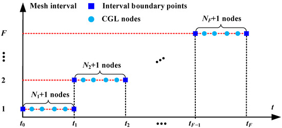
Figure 3.
Distribution of the mesh points.
From Figure 3, the time domain is divided into F sub-intervals, with boundary points and the number of mesh points in each interval is . The mesh points in the i-th interval is denoted as , where denotes the -th mesh point in the i-th mesh interval and .
For mesh points within , holds according to the PS method, and the dynamic constraints can be transformed to
where ; ; are the state and control variable at each mesh point, respectively. is the differential matrix, and the elements in can be calculated using the following equation.
where and .
Further, consider all the mesh points in the mesh interval , we have
where ; ; is the time domain conversion coefficient within each mesh interval, . and can be given by
where denotes the dimension of the state vector . denotes the Kronecker product of and identity matrix . For instance, if , we have
where are the elements in .
In addition, boundary connection constraints between mesh intervals are considered to ensure the continuity of state and control variables, which can be expressed as:
Combine Equations (11), (17), and (21), the form of the trajectory optimization problem can be converted to P2:
where is the total number of mesh intervals; is the Chebychev integral weight at the k-th mesh point in the i-th mesh interval, and the computing formula of is given by Ref. [40].
3.2. Local Mesh Refinement in Advance Based on the Violation of Path Constraints
For the problem of reentry trajectory optimization, all the path constraints have strong nonlinearity. The value of the path constraint varies non-monotonically over time, so the time corresponding to the maximum point may be located between two adjacent mesh points. When the local mesh points near the maximum value point are few, the precision of the constraint in Equation (22) is insufficient. Due to the fact that trajectory optimization based on the collocation method can only constrain the state at mesh points, the value of the non-convex path constraint is prone to exceed limits.
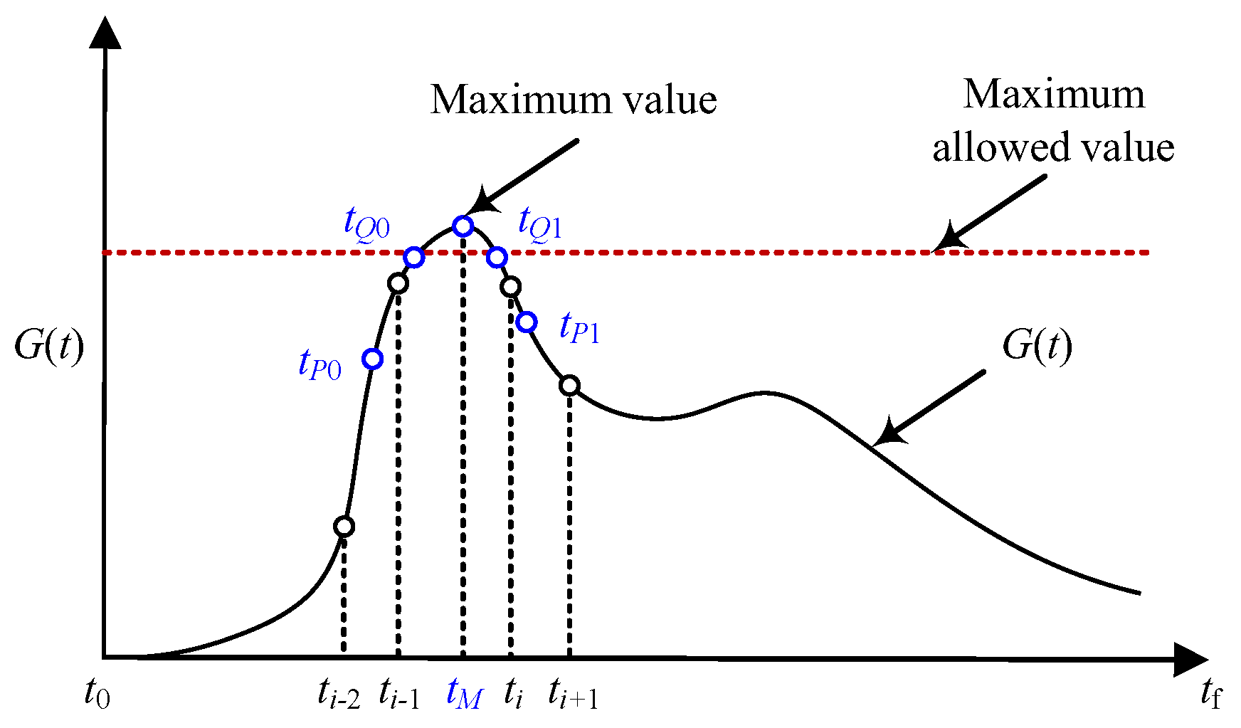
Therefore, it is necessary to refine the mesh in the vicinity of the maximum value point in advance. Figure 4 shows a schematic diagram of mesh refinement based on the violation of path constraints, and the specific process is as follows.

Figure 4.
Local mesh refinement in the vicinity of maximum value point.
Firstly, judge the constraint violation. The maximum value of the path constraint is detected, and the time when the maximum value appears is denoted as . If the maximum value is within the allowable range, there is no need to refine the mesh in advance.
Secondly, select new boundary points. If the maximum value exceeds the limit, additional mesh intervals and points are added in the vicinity of . After the location of is detected, the original mesh within the neighborhood of is refined. Taking Figure 4 as an example, as is within the i-th mesh interval , the mesh within need to be refined to enhance the satisfaction of path constraints for mesh points in the vicinity of . The mesh is refined by dividing into multiple sub-intervals. In order to determine the distribution of the sub-intervals, several mesh interval boundary points need to be added, namely and . The location of the new boundary points can be obtained by
Thirdly, generate new mesh points. Based on Equation (23), the original mesh interval have been refined into more sub-intervals . Each new sub-interval is discretized using the PS method to obtain Chebyshev–Gauss–Lobatto (CGL) points. The value of is set as the mean of the number of mesh points within the original mesh intervals.
The above process has improved the situation of constraint violations from two aspects. (1) The maximum constraint violation point is set as the boundary of the new mesh interval , and the value at can be efficiently reduced in subsequent iterations. (2) Due to the distribution characteristics of CGL points, the mesh points near are denser, which is beneficial for the satisfaction of path constraints.
3.3. Evaluation of Solution Error via Birkhoff Interpolation Polynomial
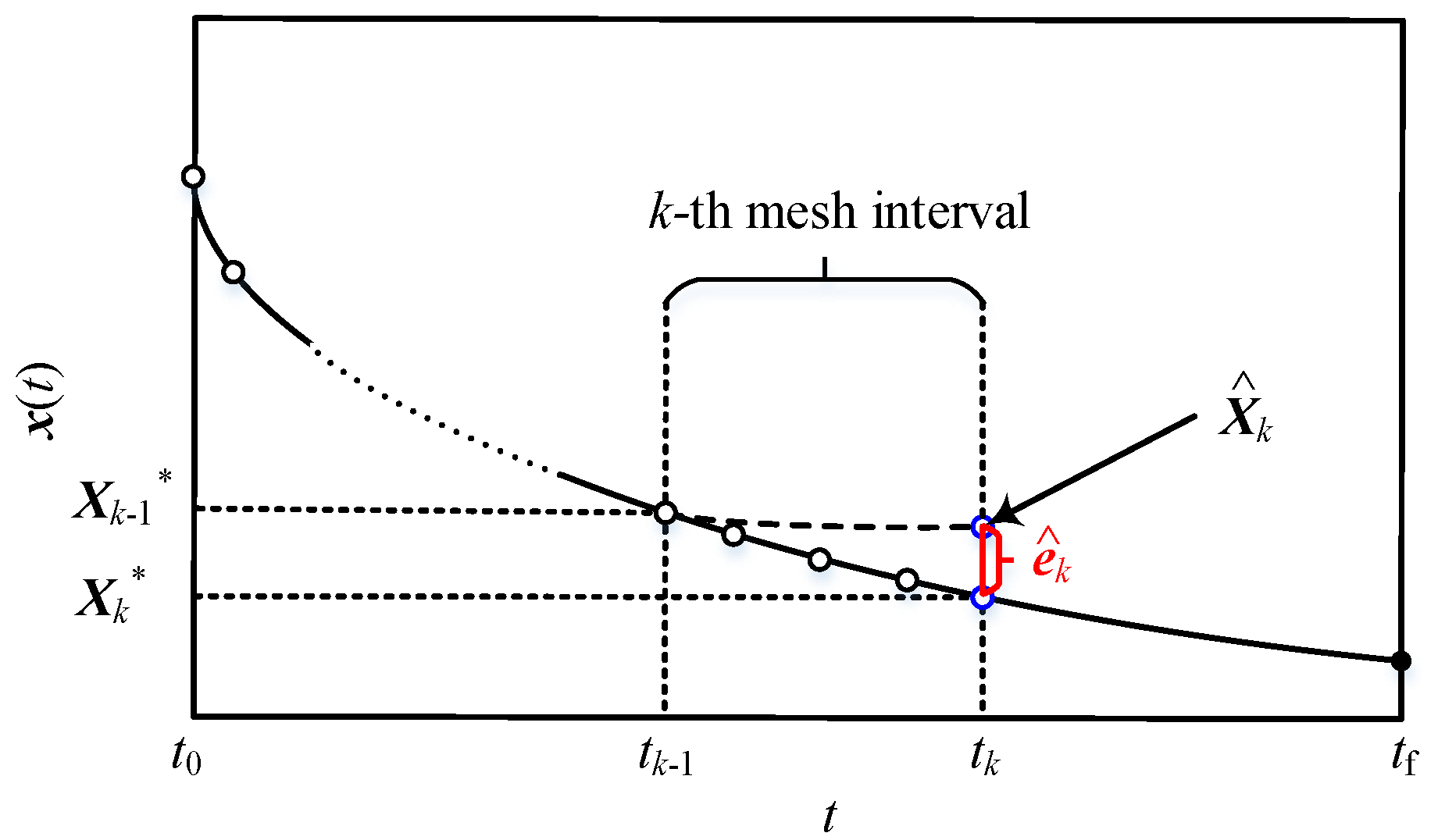
The RLV model exhibits significant nonlinearity and varies in different flight stages, making it difficult for the discrete model to accurately reflect the true dynamic characteristics. Specifically, when starting trajectory integration from the state at any mesh point until the end of the mesh interval, there will be an error between the solution and the actual state of the integral result. As shown in Figure 5, the control profile solution obtained by conventional equidistant trapezoidal discretization is verified, and the actual state at the end of the interval will deviate from the solution , resulting in state error caused by the discrete method.
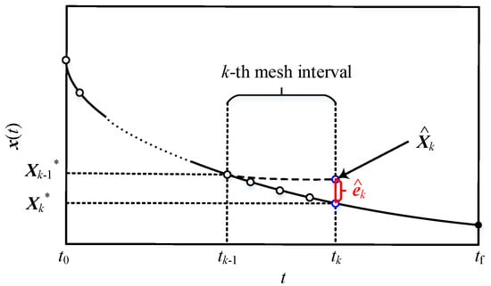
Figure 5.
Solution error of the mesh interval.
The most intuitive way to eliminate is to increase mesh points, but it will significantly increase the scale of the problem, resulting in the decrease of computational efficiency and convergence. To address the above issues, a hp-adaptive strategy with mesh reduction is proposed to capture the nonlinear characteristics of the optimization model and improve the discretization precision. The main idea is to evaluate the state error of each mesh interval based on the Birkhoff polynomial and adaptively update the mesh so as to balance the contradiction between computational efficiency and precision.
The vector composed of state solution error at each point in the k-th interval is defined as
where is the sequence of state solution in the k-th interval; is the actual state at each mesh point. In general, needs to be calculated through trajectory integration, which will consume a lot of time. In this paper, the Birkhoff interpolation polynomial is adopted to obtain explicitly.
where equals the order of the interpolation polynomial; . The coefficients of the Birkhoff interpolation polynomial satisfies
where
Thus, if of the mesh interval and is known, the state at each mesh point can be analytically calculated rapidly. To obtain , the CGL points are selected within the interval . Combined with Equation (26), it can be inferred that, , , and can be described as a matrix
where can be fitted by -order Lagrange interpolation polynomials
and
Furthermore, Equation (31) can be converted to
By combining Equations (27) and (32), it can be concluded that
where is the identity matrix; the differential matrix is given by
Then, , and can be obtained via Equation (33).
3.4. Hp-Adaptive Strategy with Mesh Reduction
On the basis of solution error evaluation, the mesh is updated based on the magnitude of solution error and state curvature within each interval. In the early stage of iteration, a certain mesh interval is divided into several sub-intervals or the number of mesh points is increased within the interval. As the solution error decreases, adjacent mesh intervals are merged based on the sliding window algorithm. The number of mesh points is reduced to improve the computational efficiency and convergence of the SCP process.
The maximum error within the interval is denoted as
where is the dimension of the state variable.
Select l CGL points within each sub-interval and calculate which represents the curvature of the p-th dimension of the state variable corresponding to
where denotes the p-th dimension of the state variable at .
Define as the ratio of the maximum state curvature at each mesh point to the average value
When , define as a preset constant, it is believed that the state variable and control variable in the interval have a high degree of nonlinearity. Thus, the interval is divided into several sub-intervals to reduce nonlinearity in each interval and improve the precision. The number of intervals within is updated by
where is a preset constant; is the expected precision.
When , it is believed that the state variable and control variable in this interval are relatively smooth, and there is no need to delineate sub-intervals. Only the number of mesh points is adjusted based on the magnitude of solution error to further improve discrete precision. Then, is updated by
where denotes the number of mesh points in the interval; is a preset constant.
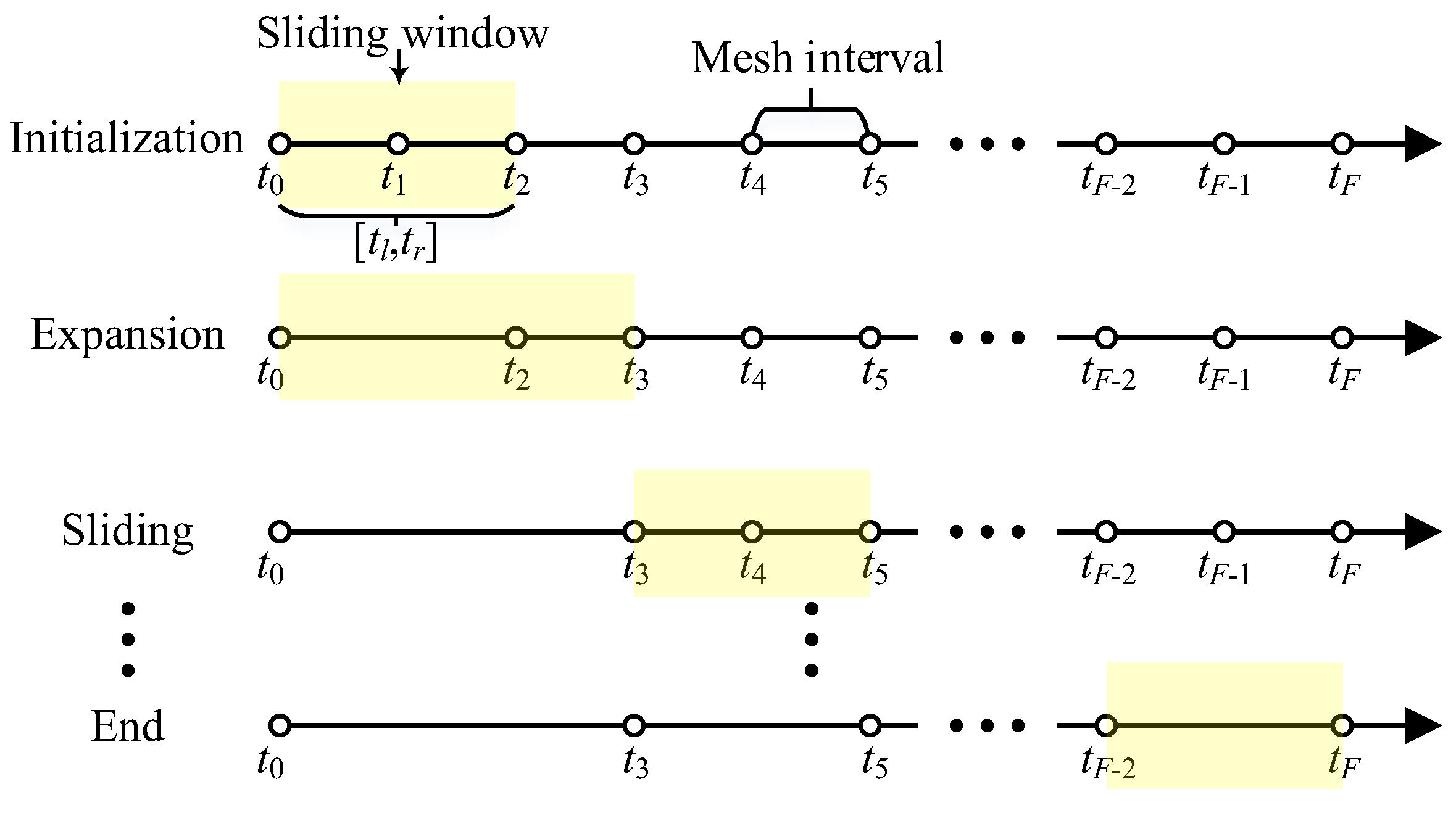
When the number of mesh intervals and points no longer increases, the mesh refinement phase is replaced by mesh reduction to reduce computational complexity. Figure 6 shows the diagram of the sliding window-based mesh reduction process.
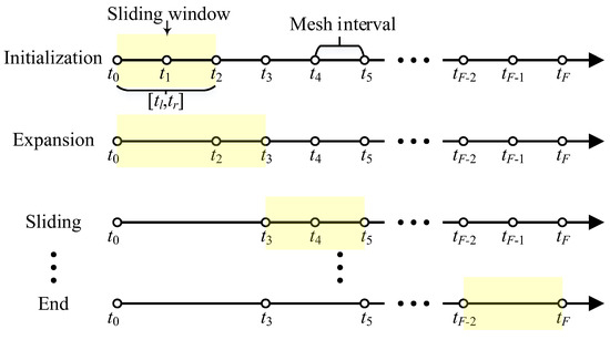
Figure 6.
The diagram of the sliding window algorithm.
Starting from the first mesh interval , three steps are alternately executed, and whether the adjacent mesh intervals can be merged is judged sequentially. Firstly, the sliding window is initialized as a time interval . and are exactly at the boundary points of the initial mesh intervals. The length of covers two intervals in the original mesh . The number of mesh points within is set as the average of and .
The maximum error within the interval is evaluated. If Equation (41) holds, and are merged, and the new interval is accepted. If not, abandon the merge and set as .
Next, assume Equation (41) holds, the coverage area of the sliding window is expanded. Set as . Recalculate within and judge whether and can be merged. If does not meet the requirements, abandon the merge and move the sliding window to the right. The length of the sliding window is reinitialized, and and are updated as
In the sliding phase, if some intervals inside the sliding window have been refined in this iteration, adjust the position of to the right to skip these intervals. As and are set, is evaluated within the new and the mesh is determined whether to merge or not. If the merging is accepted, expand the length of and continue to determine if the interval merging is possible within the new sliding window. If the merging is rejected, slide to the right and reinitialized the sliding window. Repeat the above operation until reaches the endpoint of the trajectory.
The above process can be summarized as Algorithm 2. The construction and solution process of the convex optimization problem will be provided in the next section.
| Algorithm 2. Hp-adaptive mesh refinement algorithm | |
| Input: | Initial mesh and reference solution X, the initial total number of mesh intervals F and mesh points N, preset constant parameter rmax, H1, H2 and εe, phase conversion flag for mesh refinement and mesh reduction. |
| Output: | The converged solution X(k). |
| 11: | while 1 do |
| 12: | Construct a discretized problem based on Algorithm 1 and solve the corresponding convex optimization problem via SCP. |
| 13: | if , then |
| 14: | Break; |
| 15: | end if |
| 16: | Refine the mesh in the vicinity of the maximum violation points of path constraints using Equation (23). |
| 17: | if , then |
| 18: | for i = 1: F |
| 19: | Calculate of the i-th mesh interval using Birkhoff polynomial. |
| 20: | Calculate and using Equations (38) and (39), Update F and N. |
| 21: | end for |
| 22: | If the mesh remain unchanged, set . |
| 23: | else if , then |
| 24: | while do |
| 25: | Select CGL points within a sliding window, evaluate the solution error after mesh intervals merging. |
| 26: | If , update F and N; otherwise, abandon the mesh merge. Adjust the . |
| 27: | end while |
| 28: | end if |
| 29: | end while |
| 30: | return X(k); |
4. Variable Quadratic Penalty Based SCP Method
4.1. Convexification of the Original Trajectory Optimization Model
Considering that the original problem P1 has strong non-convex characteristics, it is necessary to transform the non-convex constraint terms into convex forms, such as linear and second-order cones, in order to obtain the solution efficiently using SCP algorithms. This section focuses on the convexification of typical non-convex terms such as the objective functions, path constraints, and dynamic constraints. The specific process is as follows.
- Convexification of the objective function
The objective function is related to the state and control variables . Denote the reference trajectory in the k-th iteration as , where the superscript “(k)” represents the obtained in the (k − 1)-th iteration.
Then, the Taylor expansion of can be expressed as
where
- 2.
- Convexification of path constraints
The constraints of dynamic pressure, overload, heating rate can also be linearized near , which are related to and .
where is the partial derivative Jacobian matrix.
- 3.
- Convexification of dynamic constraint
Select new control variables as , the dynamic constraint can be organized into convex form:
where ; is the right end term of Equation (1); is related to the Earth’s rotation; is the Jacobian matrix of relative to ; ; .
When solving the trajectory solution in the k-th iteration, the previous iteration result can be substituted into . To ensure the rationality of linearization, the trust region constraint shown in Equation (47) is established.
where is a given vector.
4.2. Convex Optimization Model Based on hp Adaptive Mesh Refinement
Define the total number of mesh intervals and mesh points in the k-th iteration as hk and , respectively.
where is the number of mesh points in the i-th interval.
The optimization variables can be organized in vector form:
where denotes the vector to be optimized, and
Based on Equations (17) and (46), the convex dynamic constraint form of problem P2 under the hp-adaptive mesh refinement scheme in the k-th iteration is given by
where
and are composed of the coefficient matrices within the i-th mesh interval
Further, relax the terminal time limit to increase the optimization space. Equation (51) can be linearized as
where is the time scaling coefficient, and the total flight time can be controlled by adjusting the magnitude of .
The convex dynamic constraint with free terminal time can be given by
where ; ; .
Similarly, the path constraints can be rewritten as
where denotes the Jacobian matrix of path constraints value for ; denotes the reference value of ; denotes the limit value of .
So far, the convex optimization subproblem utilizing hp-adaptive mesh refinement can be expressed as problem P3
where are constant coefficient matrices; are used to extract the state vectors at the first and last mesh points from , respectively; are used to extract the state and control vector at the first and last mesh points within each mesh interval from .
Remark 1.
Problem P3 can be regarded as a unified problem form for the stages in the SCP algorithm. As the iteration progresses, the relaxation term and gradually approach 0. When holds, the hp-adaptive mesh refinement SCP stage begins, where and are set to 0 and the mesh is updated to improve the precision of the solution. When the number of mesh points in two adjacent iterations is less than , the mesh is considered to converge and enters the variable quadratic penalty SCP stage. The values of and need to be set based on specific problems. If the threshold is too high, it may cause the algorithm to end prematurely and the resulting mesh to not converge, thus affecting the precision of the solution. If the threshold is too small, the number of iterations may increase, reducing the computational efficiency. To balance the solution precision and computational efficiency, set ,
in this paper.
4.3. Variable Quadratic Penalty SCP Algorithm
Considering that the basic SCP algorithm is difficult to converge rapidly when dealing with strong non-convex problems, an SCP algorithm based on variable quadratic penalty is introduced in this section. The proposed algorithm consists of two stages.
In the first stage, the hard trust region-SCP algorithm is adopted. As no additional terms are introduced into the objective function, the optimality of the solution is not affected. However, this may cause the objective function to oscillate or decrease slowly around the optimal solution, and the solution process is difficult to converge. When the variation of the objective function in the adjacent four iterations satisfies Equation (61), the oscillation phenomenon is considered to occur, switch to Stage 2.
In the second stage, a variable quadratic penalty term regarding the iteration direction is introduced into the objective function. This causes the local characteristics of the objective function to be altered and can overcome the oscillation phenomenon. Simultaneously, the weight of the penalty term is dynamically adjusted according to the historical iteration direction information and the gradient at the current iteration point to improve the convergence. The specific process is as follows.
Stage 1: Hard trust region-SCP.
A general optimization problem P0 with equality and inequality constraints can be simplified as
where and represent the equality constraints and inequality constraints, respectively. and represent the number of equality and inequality constraints, respectively.
By introducing a hard trust region constraint into the objective function and combining it with P3, the convex optimization subproblem P4 can be given by
where is the gradient of the objective function obtained from the previous iteration result; are the gradients of and near the reference trajectory , respectively; is the radius of the trust region; is the iteration direction, which is the change of the current iteration optimization variable relative to
Stage 2: Iterative direction dynamic quadratic penalty-based SCP.
Step 2.1: The quadratic penalty term regarding the iteration direction is introduced into the objective function, resulting in problem P5. The coefficient of the quadratic penalty term is adaptively adjusted as the iteration progresses, so the additional term is called the variable quadratic penalty.
where is the Hessian matrix of the objective function. When the original objective function is linear or is not positive, is set as an identity matrix; is the weight of the penalty term, and its value represents the degree of dependence on the current quadratic penalty term. When is reached, P5 will degenerate to P4.
Theorem 1.
In the k-th iteration of P5, if the solution of iteration direction and the solution is a KKT solution of P5, then is also a KKT solution of the original problem P0.
Proof.
The KKT condition for P0 is given by
where is the optimal solution; and are Lagrange multipliers.
Denote the solution of P5 as , satisfying the KKT condition:
When the iteration converges, , so it is not difficult to find that the KKT condition of the original problem P0 is satisfied by . Therefore, the convergent solution of P5 is also a KKT solution of the original problem P0. This completes the proof of Theorem 1. □
According to Theorem 1, the introduction of the quadratic penalty term of iteration direction does not affect the optimality of the solution. Furthermore, and obtained from the solution are updated according to the following process.
Step 2.2: Non-monotonic filtering line search of the iteration direction.
After obtaining , a filtering set is set, and the actual solution is updated by
where is the line search parameter.
Define the initial filtering set
where c represents the violation of constraints; f is the objective function value. Starting from , a backtracking search is executed. When holds, is not accepted. When Equation (74) is established, accept .
where ; ; ; ; ; ; are positive integers.
Finally, the optimal iteration direction and the optimal solution can be obtained. The filter set is updated by
Sometimes, the value of the objective function may be lower than the optimal solution temporarily during the solving process. The basic line search requires the objective function to monotonically decrease. Hence, the solution will deviate from the optimal solution, or even no feasible solution can be found. In the non-monotonic filtering line search, the objective function value is not strictly required to monotonically decrease, but it can ensure an overall downward trend. Thus, the feasibility of the problem can be improved.
Step 2.3: Dynamic updating strategy of the quadratic penalty term coefficient .
To illustrate the adjustment strategy of , consider an optimization problem with a linear objective function [36]. The problem form for the k-th iteration is given by
where ; ; ; is the radius of trust region. It is easy to know that the optimal solution of the problem is .
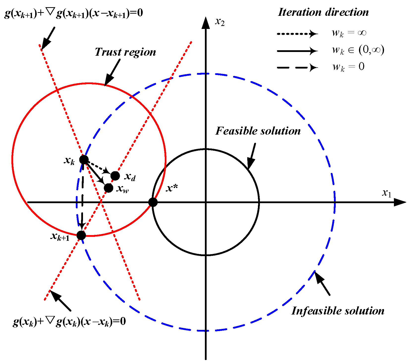
The comparison of the iteration directions of the convex optimization subproblem using hard trust region constraints and quadratic penalty terms with different weight coefficients is shown in Figure 7.
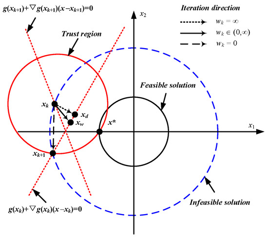
Figure 7.
Comparison of iteration directions with different objective function forms.
As shown in Figure 7, when the reference solution is denoted as , the solution should satisfy the linearized constraint . The iteration direction is defined as the vector from to . If , there is no quadratic penalty term in the objective function, and the gradient direction is the negative direction of the x1-axis, will be updated along the maximum allowable step size. Even if the optimal solution is in the range of the trust region, the solution will not converge to , but rather the intersection point between the linearized constraints and the boundaries of the trust region. At this point, although the objective function value decreases, the constraint violation is not improved. Further, at the (k + 1)-th iteration, will still fall on the trust region boundary corresponding to . The above process will be repeated, resulting in objective function oscillation and poor convergence.
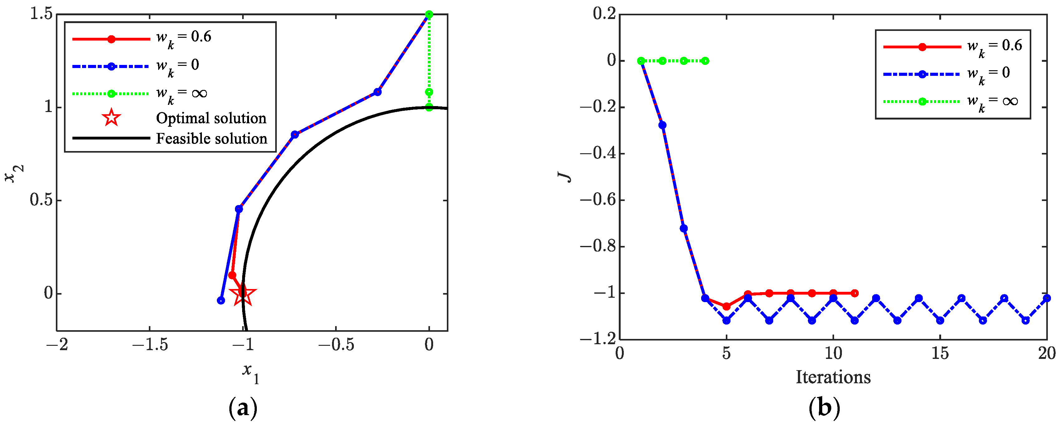
To verify the correctness of the above discussion, the SCP algorithm is used to solve the problem shown in Equation (76). Figure 8 shows the iterative histories. The five-pointed star in the figure represents the optimal solution . The black arc represents the feasible solution. The initial value of the problem solution is set as . The black arc represents the set of feasible solutions that satisfy the constraint . From the iteration histories of the solution and objective function, it can be seen that when , the convergence rate is the fastest, and the constraints are satisfied. However, the converged solution is [0, 1], which is obviously not the optimal solution. When , the objective function begins to oscillate after the 5th iteration, and the solution repeats between and , resulting in poor convergence. When , the oscillation phenomenon is eliminated after six iterations and ultimately reaches the optimal solution, which demonstrates the feasibility of the proposed method in this paper.

Figure 8.
Iteration histories for solving Equation (76) via the SCP method. (a) Histories of solution; (b) histories of objective function.
In addition, from Figure 8b, it can be observed that the objective function value increases at the 5th iteration, which is due to the previous iteration’s solution being smaller than the true optimal solution . Therefore, the algorithm tends to move the solution closer to the optimal solution. However, the basic line search algorithm requires the objective function value to be monotonically decreasing, so it fails to converge to the optimal solution. The proposed non-monotonic line search method allows for the occurrence of an increase in the value of the objective function during some iterations, thereby improving the solvability of the problem.
To overcome the oscillation, the variable quadratic penalty term is introduced in this paper. When , the effect of the original objective function can be ignored, and the iteration direction will be orthogonal to the linearization constraint, that is, will update to along the direction with the minimum distance from the linearization constraint. Thus, if is too large, will be small, and the solution will approach slowly, even converge prematurely.
In this paper, the quadratic penalty term is adaptively adjusted based on the history of gradients and iteration directions to ensure that the numerical values of and are of the same magnitude. Thus, the optimization of the original objective function and the convergence of iteration are taken into account simultaneously. is given by
where is the adaptive coefficient, which is obtained based on the history of the iteration direction. is the iteration direction obtained from the (k − 1)-th iteration. When shows an accelerating downward trend, is increased to prevent the objective function from decreasing too fast. Otherwise, is reduced to allow the original objective function to be sufficiently optimized. In general, will show a clear trend of change, which is beneficial for the algorithm. However, in some cases, if the initial startup solution is too rough, it may cause fluctuations in the value of , affecting the effectiveness of the method. At this point, a better initial startup solution should be given, or can be artificially increased to reduce the impact.
To determine the value of , define as the efficiency index
where reflects the trend of the iteration direction in two adjacent iterations. Then, is adjusted based on the second-order changes of during the iteration process.
Remark 2.
Before the adaptive adjustment of begins, is set to a constant value. In order not to affect the optimality of the solution at the beginning of the iteration, the initial value of is set to 1 in this paper. In some cases, a small may lead to an infeasible problem in the next iteration. At this point, set and solve the corresponding problem again. Iterate and adjust until the problem can be solved. In the subsequent solving process, will be automatically updated using Equations (77)–(79). In addition, in the adaptive adjustment of phase, if the objective function does not achieve a significant decrease in multiple iterations, set , which increases the value of penalty term to accelerate convergence.
The above algorithm can overcome the oscillation phenomenon of the objective function when the solution is near the optimal solution. However, how to theoretically prove the convergence of the proposed algorithm remains a difficult problem, especially when the initial starting solution is not the solution of the original problem or is far from the optimal solution. This is the future research direction of this paper.
5. Simulation and Analysis
5.1. Simulation Setting
Numerical simulation is conducted to verify the effectiveness of the proposed SCP algorithm. A vertical-takeoff horizontal-landing RLV model given in Ref. [41] is adopted. The initial and target state constraints of the RLV are listed in Table 1. The path constraints are , and . The allowable range of is . The allowable range of is . The change rate limits are and .

Table 1.
The boundary conditions of RLV.
The algorithm parameters are set as follows. The number of initial mesh intervals is 10, and the number of mesh points in each interval is 8. The mesh update parameters are , , and . The trust region parameter is and the convergence condition is set as . The weight coefficients in the objective function are , . At each iteration, a convex optimization solver called ECOS is called to solve the subproblem. The simulation is conducted on a laptop computer with AMD Ryzen 7 4800H (2.90 GHz) and Windows 10 operating system.
In Section 5.2, the solution’s effectiveness and precision are demonstrated. The proposed method is compared with the hp-adaptive PS-SCP method and the basic SCP method in terms of solution precision, optimality, and computational efficiency. In Section 5.3, the convergence process of the proposed method is given. The proposed method is compared with different trust region-based SCP methods, and the effect of the penalty coefficient is analyzed. Finally, no-fly zone constraints are considered to validate the algorithm’s adaptability to complex scenarios.
5.2. Simulation Analysis of Algorithm Precision
In this section, the effectiveness and precision of the proposed algorithm are verified. Firstly, the comparison between the discrete solution and the integral solution obtained via the proposed method is given, as well as the curves of path constraints. Next, P5 is solved using different methods, which are the proposed method in this paper, the hp-adaptive PS-SCP method (excluding mesh reduction), and the basic SCP methods with a different total number of mesh points. The basic SCP methods use a fixed uniform grid, and the number of mesh points is consistent with the first two methods, respectively.
The specific simulation results are as follows.
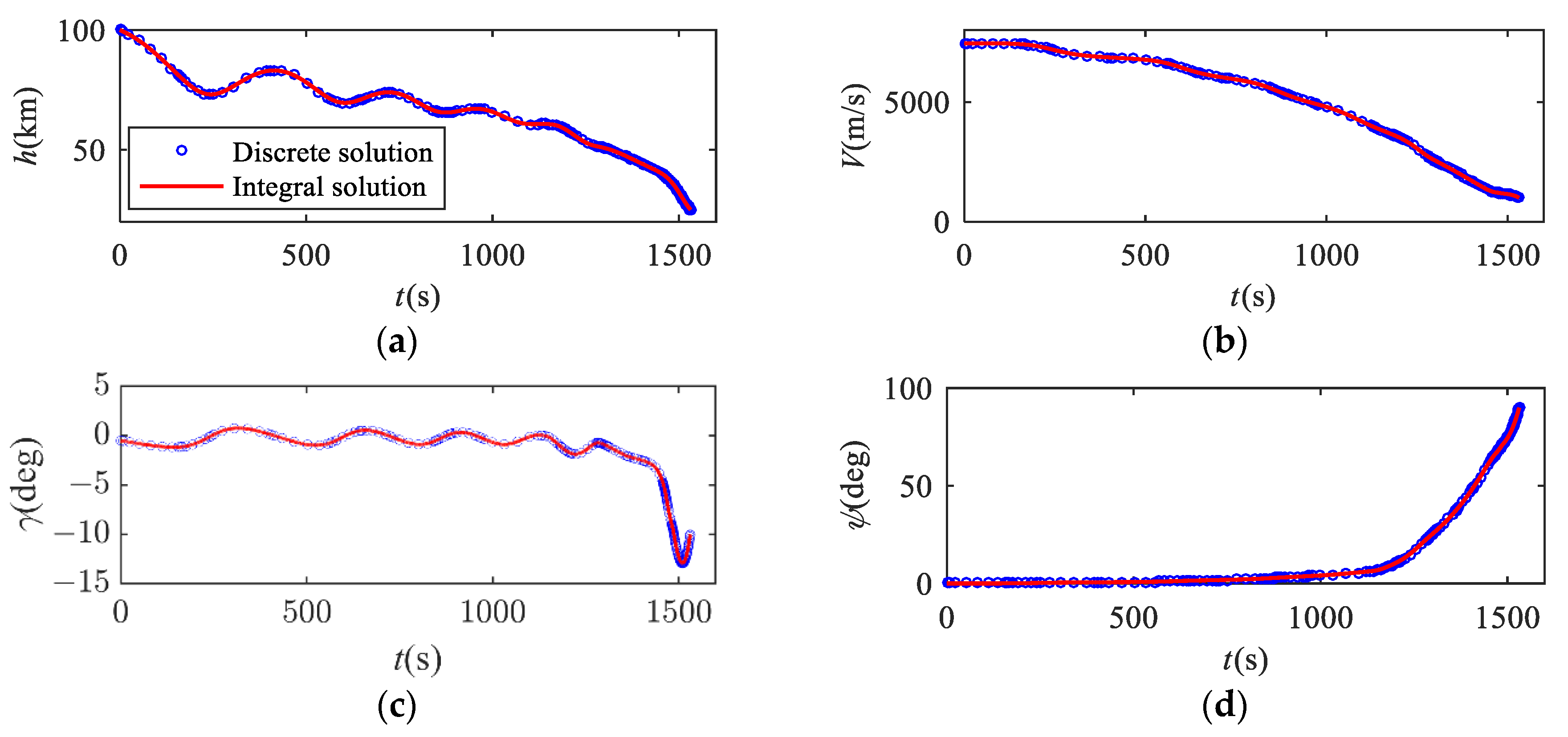
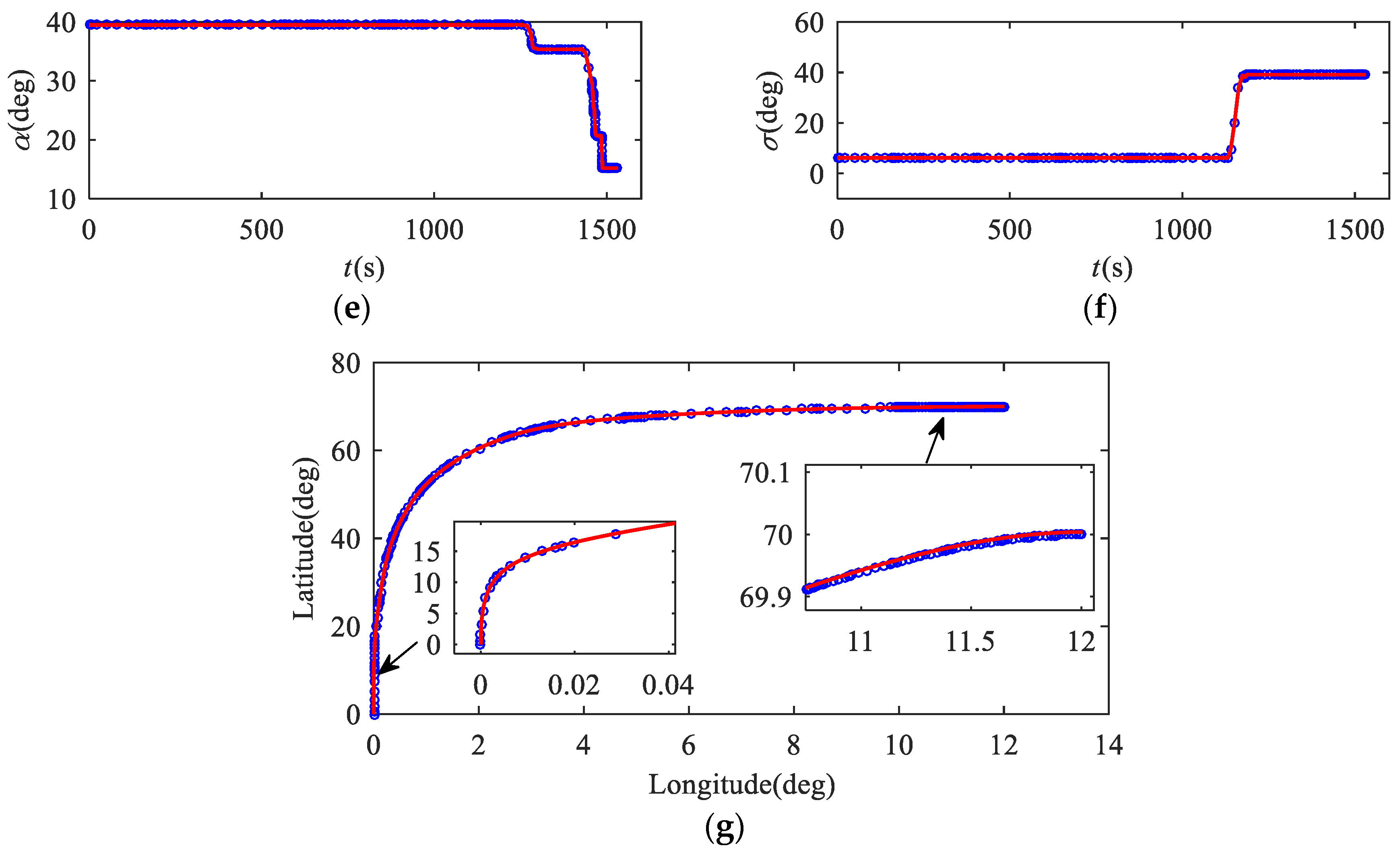
Figure 9 shows the comparison of the discrete solution and the integral solution. The discrete solution represents the trajectory solution obtained by the proposed method, while the integral solution represents the results obtained by trajectory integration using the actual dynamic model. The solution error is defined as the terminal state deviation between the discrete solution and the integral solution, and the magnitude of the solution error reflects the precision of the method. According to Figure 9g, the distribution of mesh points is non-uniform. The mesh points are denser in cases where the curvature of the state variables is larger and at the end of the trajectory. These parts have strong nonlinearity, and the solution precision is improved by more mesh points.
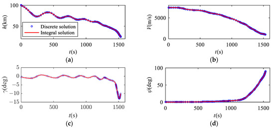
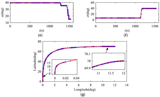
Figure 9.
Comparison of discrete solution and integral solution. (a) Curves of height; (b) curves of velocity; (c) curves of flight path angle; (d) curves of heading angle; (e) curves of attack angle; (f) curves of bank angle; (g) curves of ground track.
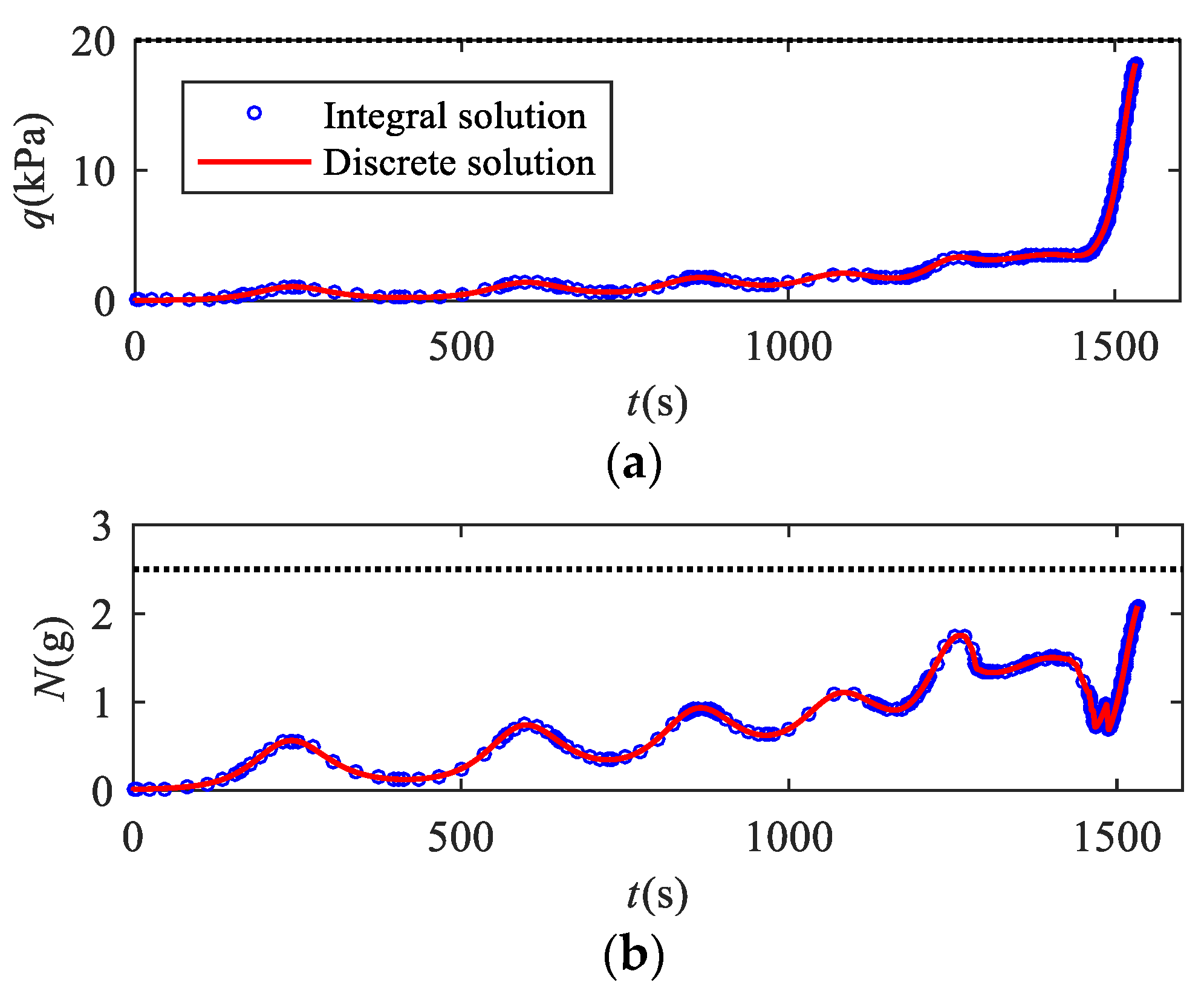
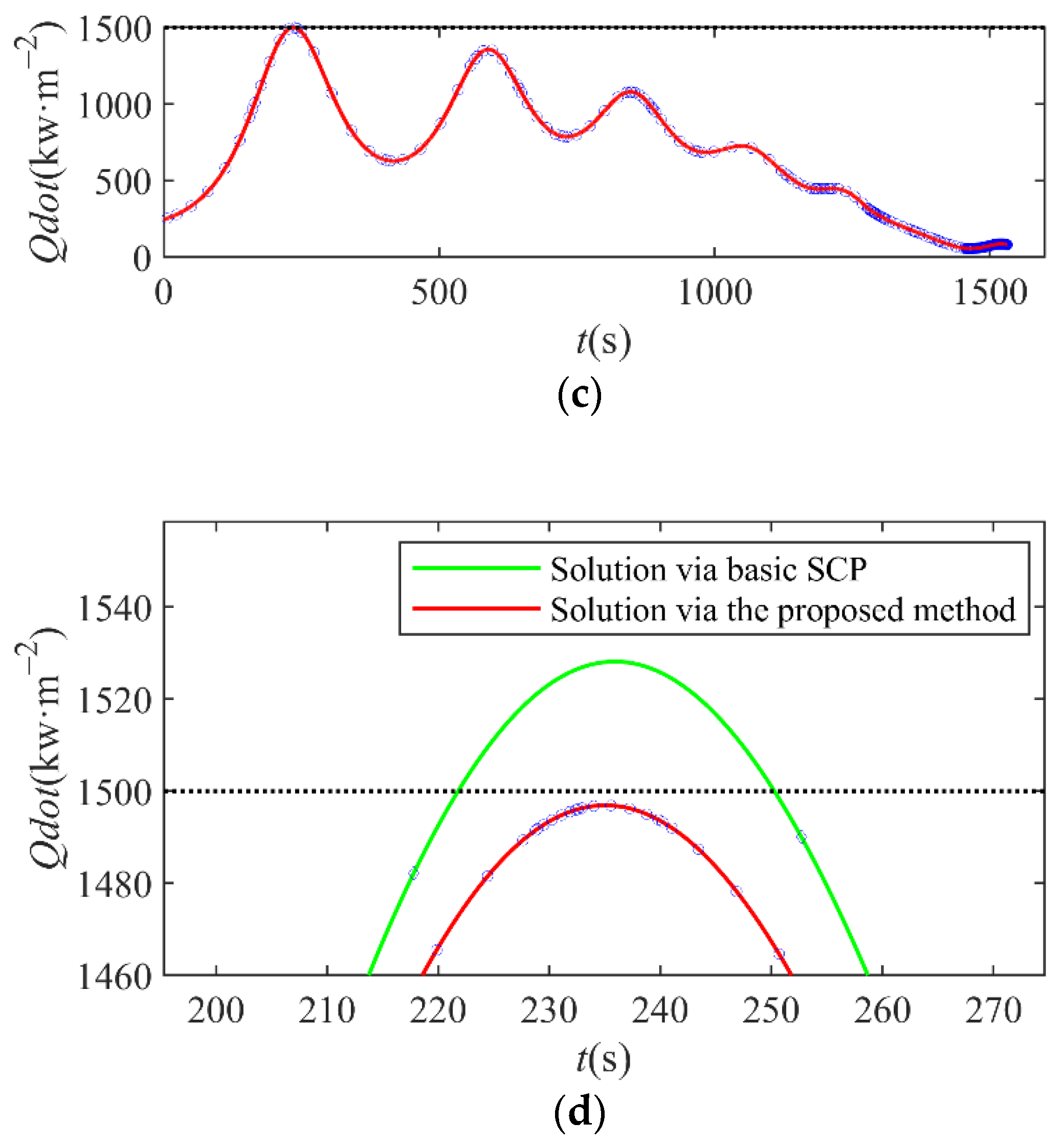
Figure 10 shows the variation of dynamic pressure, overload, and heating rate on the RLV over time. The black dashed line represents the maximum allowable value, indicating that all path constraints are within a reasonable range. In addition, the mesh points are denser in the vicinity of the extremum value points of the curve of and , which prevents path constraints from exceeding limits. From Figure 10d, we can know that the maximum value point of may exist between two adjacent mesh points during the iterations. When the mesh points are few near the maximum point, will slightly exceed the limit. By utilizing the proposed method, the mesh is refined in the vicinity of the maximum point, which improves the satisfaction of the non-convex path constraints.
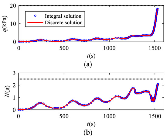
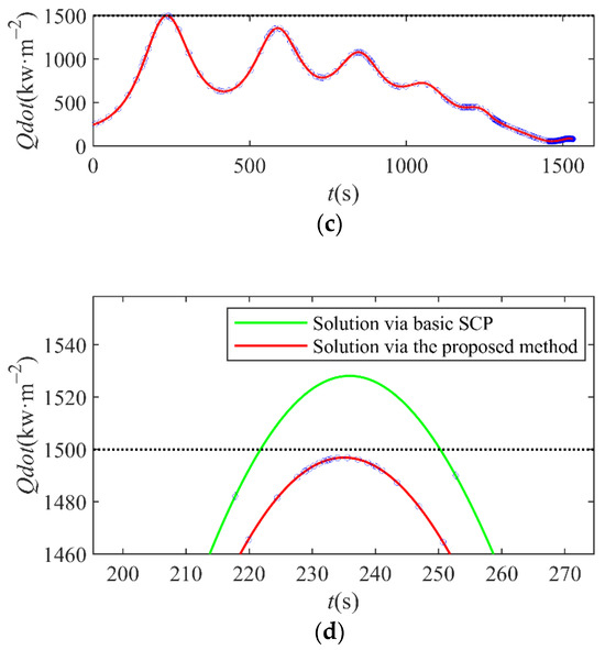
Figure 10.
Path constraints–time curves. (a) Curves of dynamic pressure; (b) curves of overload; (c) curves of heating rate; (d) comparison of the curves of heating rate in the 5th iteration via the proposed method and the basic method without consideration of constraints violation.
The trajectory solution statistics results corresponding to different methods are shown in Table 2. It can be seen that the proposed method has high terminal precision. The terminal height error is less than 30 m, velocity error is less than 10 m/s, and latitude and longitude errors are less than 0.01°. Compared with uniform discretization-based basic SCP methods, the errors in flight path angle and heading angle are both small and the precision is improved by an order of magnitude. The hp-adaptive PS-SCP method does not utilize mesh reduction, and the number of mesh points after convergence is more than twice that of the proposed method. The number of iterations also increases, which leads to an increase in time consumption. However, compared to the mesh reduction method proposed in this paper, using more mesh points cannot significantly reduce the terminal state error of the solution. In terms of objective function optimization, the proposed method is consistent with the hp-adaptive PS-SCP method, and both are superior to the basic SCP methods. In terms of solving efficiency, the conventional hp-adaptive PS-SCP method takes the longest time, while the basic SCP method takes the shortest time. The proposed method reduces the total solving time by 45% while maintaining comparable precision to the hp-adaptive PS-SCP method. Thus, the proposed method can be seen as a compromise approach that balances computational efficiency and precision.
Table 2.
Solution statistics results.
5.3. Simulation Analysis of Algorithm Convergence Process
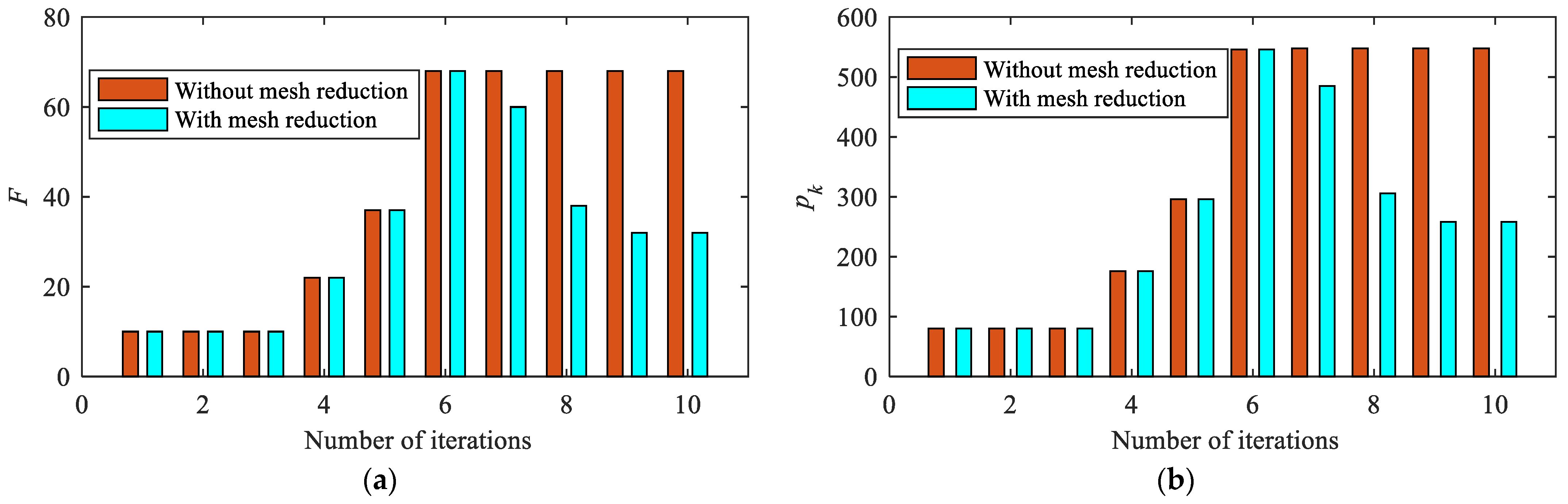
Figure 11 shows the histories of mesh intervals and points using hp-adaptive mesh refinement and the proposed method. In the initial mesh, the number of mesh intervals and the number of discrete points . Due to the fact that the first three iterations are SCP processes with relaxed constraints, and of the mesh is fixed. In the hp-adaptive mesh refinement phase, and increase until the 7th iteration. At this point, the mesh corresponding to the conventional method without mesh reduction has converged, and a fixed mesh () will be used for solving the trajectory. In comparison, the mesh reduction starts to be implemented using the proposed method, and the number of mesh intervals and discrete points rapidly decreases until the 10th iteration. The mesh can converge () with only three additional times of mesh error evaluation and update, which will reduce the complexity and time consumption of the solution process efficiently.
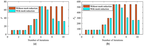
Figure 11.
Histories of mesh intervals and points using hp-adaptive mesh refinement and the proposed method. (a) Histories of the number of mesh intervals; (b) histories of the number of mesh points.
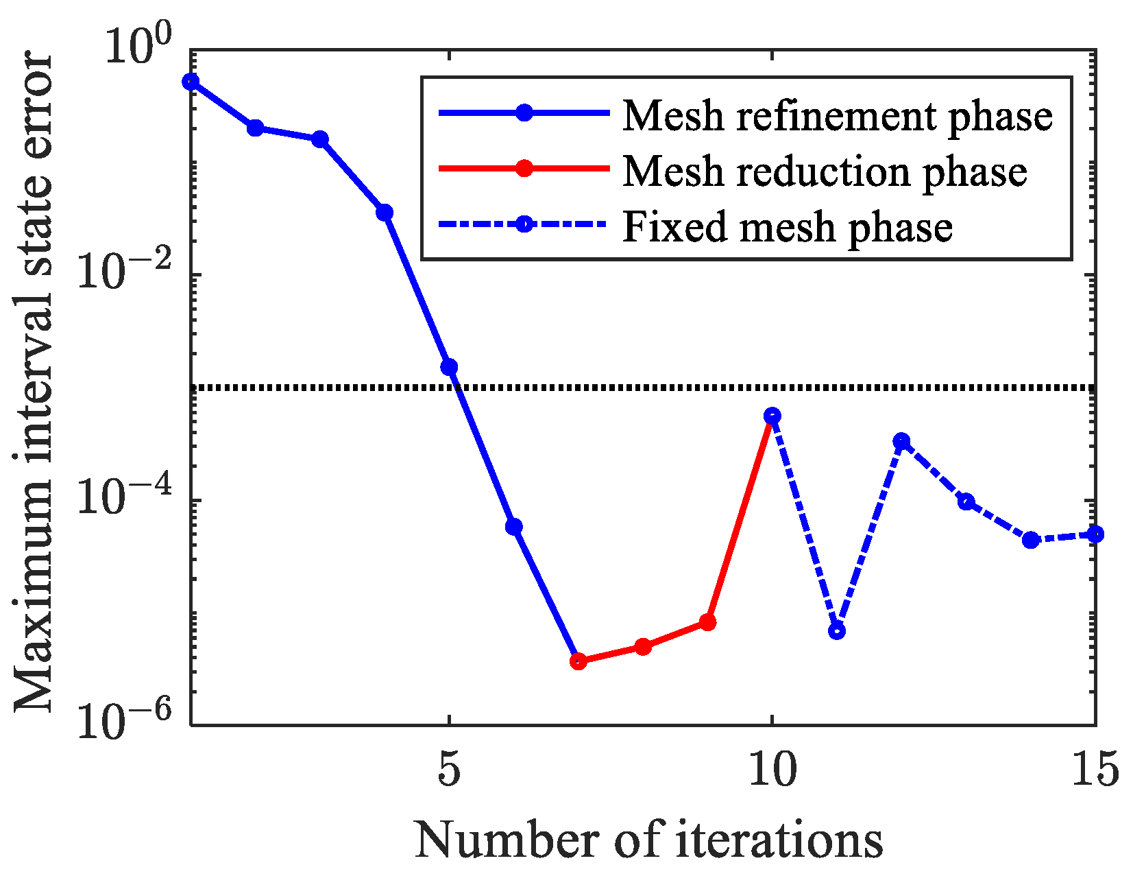
Figure 12 shows the statistical results of the maximum state error of all mesh intervals in each iteration. As and are adjusted during the mesh refinement phase, gradually decreases. After eight iterations, is satisfied in all subsequent iterations, and the discretization precision within all mesh intervals meets the constraints even if the mesh is no longer being updated.
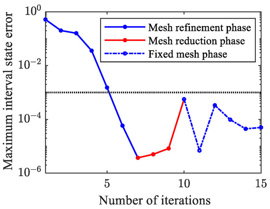
Figure 12.
Histories of maximum interval state error.
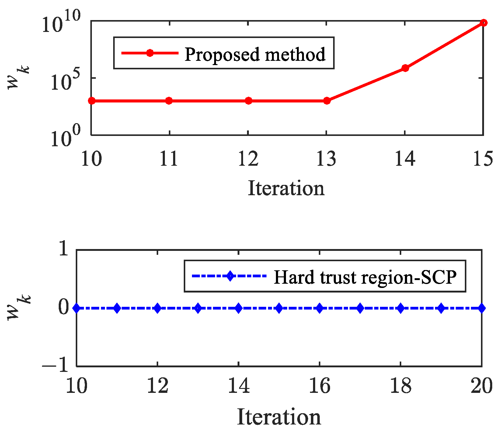
Figure 13 and Figure 14 show the histories of objective function value and using the proposed method and hard trust region-SCP. After 10 iterations, the mesh converges, and the fixed mesh solution phase starts. It can be observed that the objective function is not monotonically decreased; the oscillation phenomenon occurs. The hard trust region SCP method does not introduce a quadratic penalty term (), and the solution process has not converged after 20 iterations. It should be noted that although the oscillation amplitude of is not large after the 15th iteration, this does not mean convergence, and the precision of the solution is quite low. In other words, if the control profile obtained by the hard trust region SCP method is substituted into the actual dynamic system for numerical integration, the terminal state will deviate significantly from the target value.
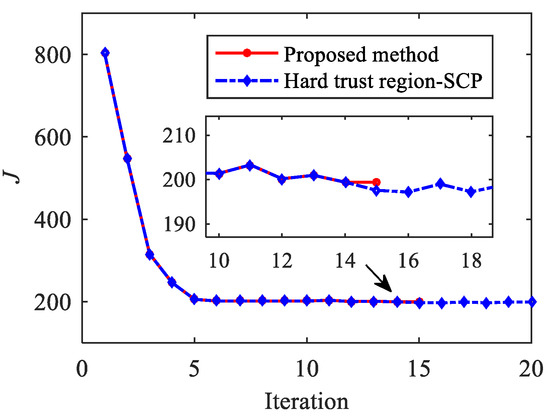
Figure 13.
Histories of objective function value.

Figure 14.
Histories of .
In comparison, the proposed method detected the oscillation phenomenon at the 13th iteration, a quadratic penalty term is introduced into the objective function, and the coefficient of the penalty term is adaptively adjusted in the following iterations, which is beneficial for the convergence.
In order to verify the effectiveness of the variable quadratic penalty term, further comparative simulations of different methods are conducted under fixed uniform mesh conditions, and the influence of penalty function coefficients on the convergence process is analyzed. The total flight time corresponding to the initial iteration value is set to 1600 s. The setting of the objective function and constraint conditions is the same as before.
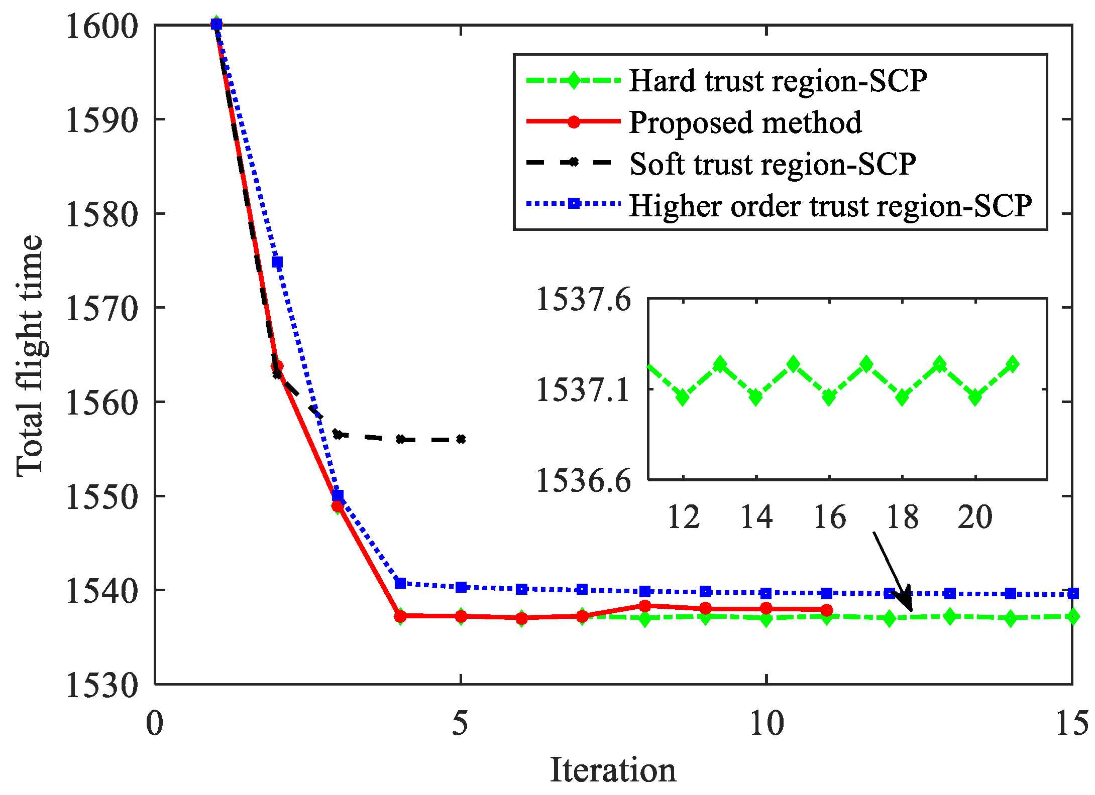
Figure 15 shows the history of the total flight time using different methods. The soft trust region-SCP method can converge after five iterations, which has the fastest convergence speed. However, compared to other methods, the objective function of the convergent solution has not been sufficiently reduced, and its optimality is poor. Although the high-order trust region SCP method has optimality in theory, simulation results show that the update step size of the solution is very small after four iterations, and the objective function decreases slowly. After 20 iterations, it still does not converge. The hard trust region-SCP method has the fastest descent rate of the objective function in the early phase, but after five iterations, an oscillation phenomenon occurs, making it unable to converge.
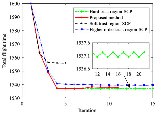
Figure 15.
Histories of total flight time.
In contrast, the proposed method overcomes the oscillation phenomenon and converges after 11 iterations. Under the same terminal state precision conditions, the performance index obtained by the proposed method is better than those obtained by the soft trust region-SCP and hard trust region-SCP methods. It should be noted that although the hard trust region-SCP method obtains a smaller objective function value, the terminal height error exceeds 1 km, and the speed error is greater than 100 m/s, so it is not the feasible solution to the original problem.
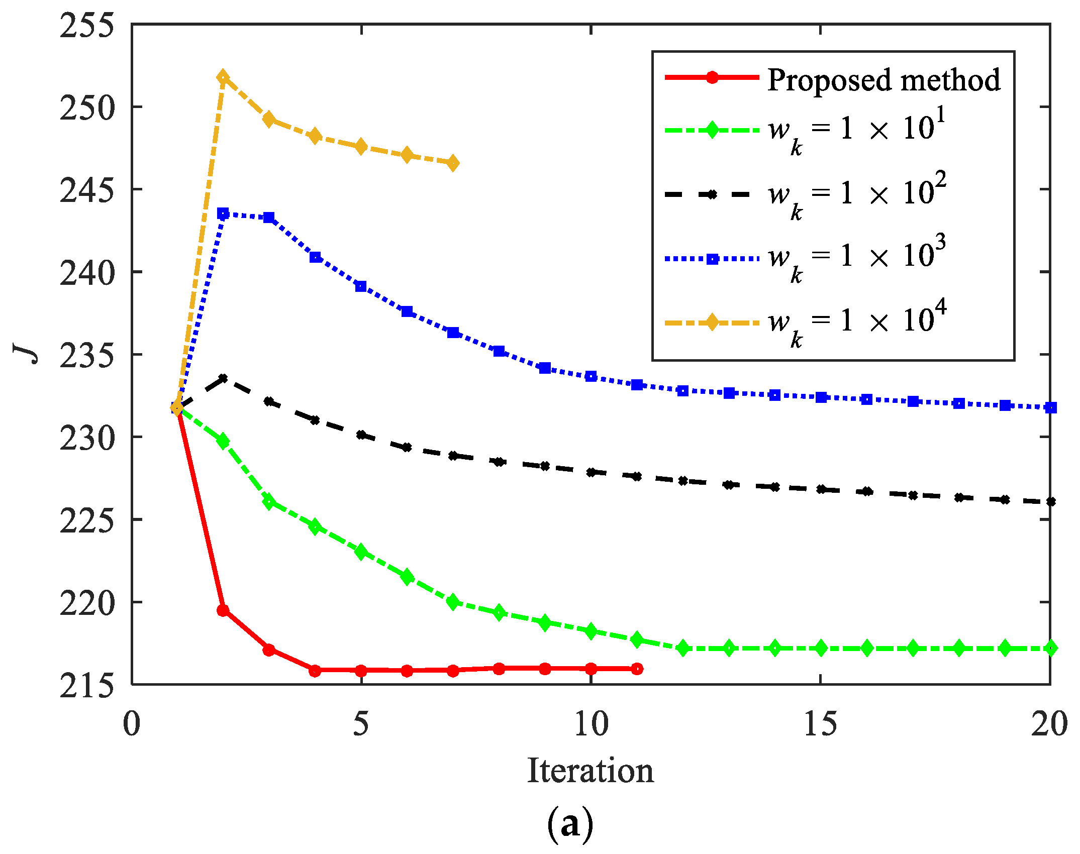
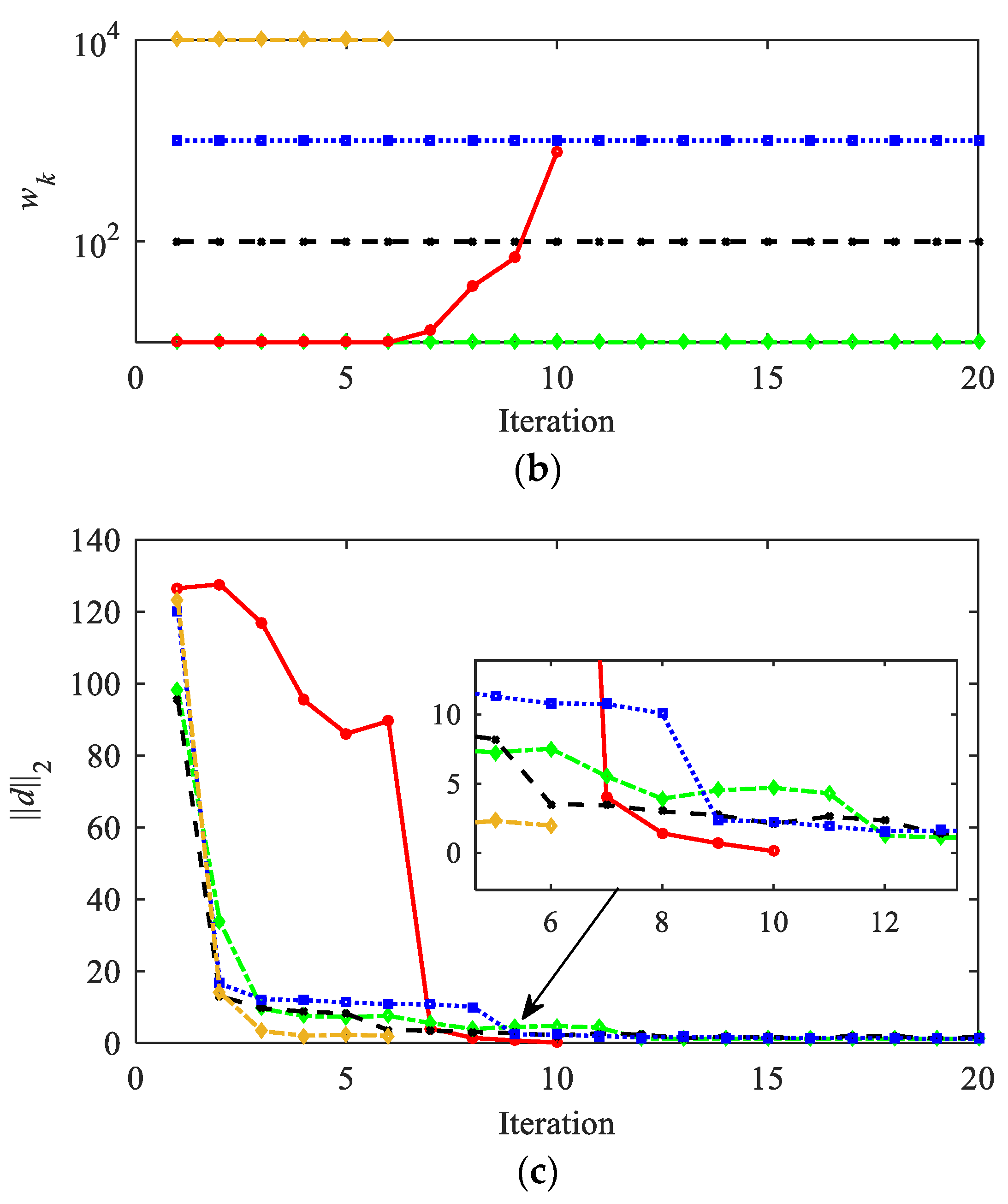
Figure 16 shows the comparison of the convergence process under different penalty coefficients. The red solid line in the figure represents the variable coefficient method proposed in this paper, while other curves represent the fixed coefficient method. The legend provides the specific value of the fixed coefficient. As shown in Figure 16, different penalty coefficients will have a significant impact on the descent process of the objective function. The smaller the is, the faster J decreases in the early stages of the iteration, which is more advantageous for the optimality of the results. However, if remains at a small value, such as , oscillation will still occur in the later stages of iteration. When is greater than 1 × 10², J first increases and then gradually decreases. Although larger can suppress oscillation phenomenon and J monotonically decreases, the descent speed is slow in the later stages of iteration, resulting in poor convergence. Meanwhile, an excessively large will cause to quickly approach 0, significantly reducing the number of iterations at the cost of a decrease in the optimality. The proposed method has a small value of in the early stage of iteration, which leads to a rapid decrease in J. In the later stage of iteration, the value of is adaptively adjusted to accelerate convergence. Therefore, convergence and optimality are simultaneously considered.
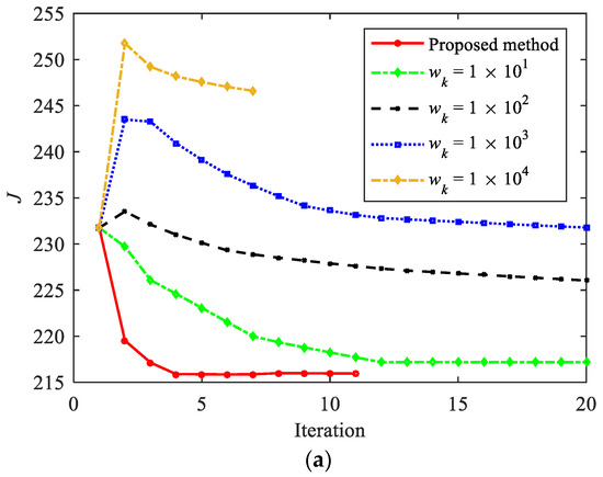

Figure 16.
Iteration histories using different penalty coefficient . (a) Histories of objective function value; (b) histories of penalty coefficient ; (c) histories of .
To validate the proposed method’s adaptability to more complex scenarios, we extended the trajectory planning to incorporate multiple no-fly zones. The simulation settings remain consistent with those in Section 5.1. Two circular no-fly zones are considered, with centers at points and , both having a radius of 2°. The no-fly zone constraints can be expressed as follows.
where are the longitude and latitude of the no-fly zone center. is the radius of the no-fly zone. By incorporating Equation (80) into problem P2 and applying the SCP algorithm developed in this paper, the trajectory results are obtained as follows.
In Figure 17, the cylinder represents the no-fly zone considered in this paper. From the 3D trajectory obtained, it can be seen that the trajectory optimization results can effectively ensure the avoidance of multiple no-fly zones. From Figure 18, it can be seen that the control variable changes smoothly with time. In addition, after integration verification of the optimization results, the terminal height error is 4.76 m, the terminal speed error is 0.90 m/s, the terminal latitude and longitude error is less than 0.01°, and the terminal heading angle and path angle errors are both less than 0.1°. Therefore, the precision of the trajectory optimization results meets the requirements, and the proposed method can adapt to complex constrained reentry scenarios containing multiple no-fly zones.
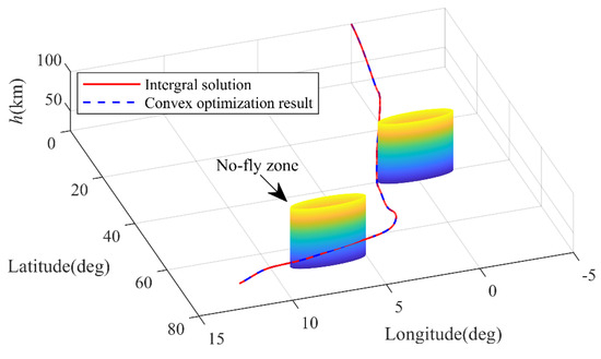
Figure 17.
The 3D trajectory results under no-fly zone constraints.
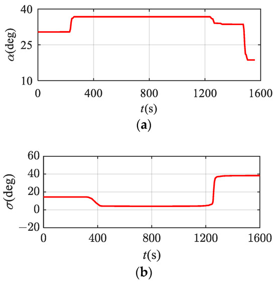
Figure 18.
Control variable curves under no-fly zone constraints. (a) Curve of attack angle; (b) curve of bank angle.
6. Conclusions
In this paper, an SCP method utilizing modified hp-adaptive mesh refinement and variable quadratic penalty is proposed to improve the computational efficiency and convergence for reentry trajectory optimization of RLVs. The conclusion is summarized as follows:
- (1)
- The modified hp-adaptive PS discretization method for reentry trajectory optimization is proposed. By accurately detecting the violation points of path constraints, additional mesh points are added in the vicinity of these violation points, which improves the satisfaction of non-convex constraints;
- (2)
- The mesh reduction phase is introduced into the hp-adaptive framework. The mesh intervals within a sliding window are merged according to discrete state error, which is evaluated by the Birkhoff polynomial explicitly. The required mesh points are reduced under certain precision;
- (3)
- The variable quadratic penalty-based SCP algorithm is proposed for improving convergence. The quadratic penalty coefficient is adjusted to avoid premature or slow convergence, which is beneficial for balancing the solution optimality and convergence;
- (4)
- Numerical simulation shows that the scale of convex optimization subproblems can be significantly reduced while meeting accuracy requirements. The total solving time has been reduced compared to the conventional hp-adaptive SCP method. In addition, the variable quadratic penalty can effectively overcome the oscillation phenomenon of the objective function. The computational efficiency and convergence of the SCP algorithm have been improved.
Author Contributions
Methodology, Z.L. and N.C.; Validation, Z.L.; Investigation, L.D. and J.P.; Writing—original draft, Z.L.; Writing—review and editing, L.D. and J.P.; Supervision, N.C. and J.P. All authors have read and agreed to the published version of the manuscript.
Funding
This research was funded by the National Natural Science Foundation of China (grant number 62373124) and the National Natural Science Foundation of China Joint Fund (grant number U2241215).
Data Availability Statement
Data are contained within the article.
Conflicts of Interest
The authors declare no conflicts of interest.
References
- Hui, X.; Cai, G.; Zhang, S.; Yang, X.; Hou, M. Hypersonic reentry trajectory optimization by using improved sparrow search algorithm and control parametrization method. Adv. Space Res. 2022, 69, 2512–2524. [Google Scholar] [CrossRef]
- Mishra, D.; Gangireddy, S. A novel re-entry trajectory design strategy enforcing inequality and terminal constraints in height-velocity plane. Adv. Space Res. 2024, 73, 2515–2531. [Google Scholar] [CrossRef]
- Zhang, W.; Chen, W.; Yu, W. Analytical solutions to three-dimensional hypersonic gliding trajectory over rotating Earth. Acta Astronaut. 2021, 179, 702–716. [Google Scholar] [CrossRef]
- Mall, K.; Taheri, E. Three-Degree-of-Freedom Hypersonic Reentry Trajectory Optimization Using an Advanced Indirect Method. J. Spacecr. Rockets 2022, 59, 1463–1474. [Google Scholar] [CrossRef]
- Zhang, R.; Xie, Z.; Wei, C.; Cui, N. An enlarged polygon method without binary variables for obstacle avoidance trajectory optimization. Chin. J. Aeronaut. 2023, 36, 284–297. [Google Scholar] [CrossRef]
- Zhao, D.; Song, Z. Reentry trajectory optimization with waypoint and no-fly zone constraints using multiphase convex programming. Acta Astronaut. 2017, 137, 60–69. [Google Scholar] [CrossRef]
- Jansson, O.; Harris, M. Convex optimization-based techniques for trajectory design and control of nonlinear systems with polytopic range. Aerospace 2023, 10, 71. [Google Scholar] [CrossRef]
- Li, W.; Li, W.; Cheng, L.; Gong, S. Trajectory optimization with complex obstacle avoidance constraints via homotopy network sequential convex programming. Aerospace 2022, 9, 720. [Google Scholar] [CrossRef]
- Shen, Z.; Zhou, G.; Huang, H.; Huang, C.; Wang, Y.; Wang, F. Convex optimization-based trajectory planning for quadrotors landing on aerial vehicle carriers. IEEE Trans. Intell. Veh. 2024, 9, 138–150. [Google Scholar] [CrossRef]
- Kumagai, N.; Kenshiro, O. Adaptive-mesh sequential convex programming for space trajectory optimization. J. Guid. Contr. Dyn. 2024, 1–8. [Google Scholar] [CrossRef]
- Dai, P.; Feng, D.; Feng, W.; Cui, J.; Zhang, L. Entry trajectory optimization for hypersonic vehicles based on convex programming and neural network. Aerosp. Sci. Technol. 2023, 137, 108259. [Google Scholar] [CrossRef]
- Liu, C.; Zhang, C.; Xiong, F.; Wang, J. Multi-stage trajectory planning of dual-pulse missiles considering range safety based on sequential convex programming and artificial neural network. Part. G J. Aerosp. Eng. 2022, 237, 1449–1463. [Google Scholar] [CrossRef]
- Açıkmeşe, B.; Blackmore, L. Lossless convexification of a class of optimal control problems with non-convex control constraints. Automatica 2011, 47, 341–347. [Google Scholar] [CrossRef]
- Acikmese, B.; Ploen, S. Convex Programming Approach to Powered Descent Guidance for Mars Landing. J. Guid. Contr. Dyn. 2007, 30, 1353–1366. [Google Scholar] [CrossRef]
- Wang, Z.; Grant, M. Constrained Trajectory Optimization for Planetary Entry via Sequential Convex Programming. J. Guid. Contr. Dyn. 2017, 40, 2603–2615. [Google Scholar] [CrossRef]
- Cheng, X.; Li, H.; Zhang, R. Autonomous trajectory planning for space vehicles with a Newton–Kantorovich/convex programming approach. Nonlinear Dyn. 2017, 89, 2795–2814. [Google Scholar] [CrossRef]
- Zhang, T.; Su, H.; Gong, C. A three-stage sequential convex programming approach for trajectory optimization. Aerosp. Sci. Technol. 2024, 149, 109128. [Google Scholar] [CrossRef]
- Zhao, J.; Li, S. Modified Multiresolution Technique for Mesh Refinement in Numerical Optimal Control. J. Guid. Contr. Dyn. 2017, 40, 3328–3338. [Google Scholar] [CrossRef]
- Zhao, J.; Li, S. Mars atmospheric entry trajectory optimization with maximum parachute deployment altitude using adaptive mesh refinement. Acta Astronaut. 2019, 160, 401–413. [Google Scholar] [CrossRef]
- Liu, F.; Hager, W.; Rao, A. Adaptive mesh refinement method for optimal control using non smoothness detection and mesh size reduction. J. Franklin. Inst. 2015, 352, 4081–4106. [Google Scholar] [CrossRef]
- Zhou, X.; He, R.; Zhang, H.; Tang, G.; Bao, W. Sequential convex programming method using adaptive mesh refinement for entry trajectory planning problem. Aerosp. Sci. Technol. 2021, 109, 106374. [Google Scholar] [CrossRef]
- Benson, D.; Huntington, G.; Thorvaldsen, T.; Rao, A. Direct Trajectory Optimization and Costate Estimation via an Orthogonal Collocation Method. J. Guid. Contr. Dyn. 2006, 29, 1435–1440. [Google Scholar] [CrossRef]
- Koeppen, N.; Ross, I.; Wilcox, L.; Proulx, R. Fast Mesh Refinement in Pseudospectral Optimal Control. J. Guid. Contr. Dyn. 2019, 42, 711–722. [Google Scholar] [CrossRef]
- Zhang, Z.; Zhao, D.; Li, X.; Kong, C.; Su, M. Convex Optimization for Rendezvous and Proximity Operation via Birkhoff Pseudospectral Method. Aerospace 2022, 9, 505. [Google Scholar] [CrossRef]
- Darby, C.; Hager, W.; Rao, A. Direct Trajectory Optimization Using a Variable Low-Order Adaptive Pseudospectral Method. J. Spacecr. Rockets 2011, 48, 433–445. [Google Scholar] [CrossRef]
- Han, P.; Shan, J.; Meng, X. Re-entry trajectory optimization using an hp-adaptive Radau pseudospectral method. P. I. Mech. Eng. Part. G. J. Aerosp. Eng. 2012, 227, 1623–1636. [Google Scholar] [CrossRef]
- Zhao, J.; Li, J.; Li, S. Low-Thrust Transfer Orbit Optimization Using Sequential Convex Programming and Adaptive Mesh Refinement. J. Spacecr. Rockets. 2023, 61, 1–18. [Google Scholar] [CrossRef]
- Zhang, T.; Su, H.; Gong, C. hp-Adaptive RPD based sequential convex programming for reentry trajectory optimization. Aerosp. Sci. Technol. 2022, 130, 107887. [Google Scholar] [CrossRef]
- Liu, X.; Shen, Z.; Lu, P. Solving the maximum-crossrange problem via successive second-order cone programming with a line search. Aerosp. Sci. Technol. 2015, 47, 10–20. [Google Scholar] [CrossRef]
- Wang, Z.; McDonald, S. Convex relaxation for optimal rendezvous of unmanned aerial and ground vehicles. Aerosp. Sci. Technol. 2020, 99, 105756. [Google Scholar] [CrossRef]
- Wang, Z. Optimal trajectories and normal load analysis of hypersonic glide vehicles via convex optimization. Aerosp. Sci. Technol. 2019, 87, 357–368. [Google Scholar] [CrossRef]
- Wang, Z.; Lu, Y. Improved Sequential Convex Programming Algorithms for Entry Trajectory Optimization. J. Spacecr. Rockets 2020, 57, 1373–1386. [Google Scholar] [CrossRef]
- Gao, Y.; Shao, Z.; Song, Z. Enhanced Successive Convexification Based on Error-Feedback Index and Line Search Filter. J. Guid. Contr. Dyn. 2022, 45, 2243–2257. [Google Scholar] [CrossRef]
- Reynolds, T.; Mehran, M. The Crawling Phenomenon in Sequential Convex Programming. In Proceedings of the American Control Conference, Denver, CO, USA, 1–3 July 2020. [Google Scholar]
- Lu, P. Convex–Concave Decomposition of Nonlinear Equality Constraints in Optimal Control. J. Guid. Contr. Dyn. 2021, 44, 4–14. [Google Scholar] [CrossRef]
- Xie, L.; He, R.; Zhang, H.; Tang, G. Oscillation Phenomenon in Trust-Region-Based Sequential Convex Programming for the Nonlinear Trajectory Planning Problem. IEEE Trans. Aerosp. Electron. Syst. 2022, 58, 3337–3352. [Google Scholar] [CrossRef]
- Xie, L.; Zhou, X.; Zhang, H.; Tang, G. Higher-Order Soft-Trust-Region-Based Sequential Convex Programming. J. Guid. Contr. Dyn. 2023, 46, 2199–2206. [Google Scholar] [CrossRef]
- Xie, L.; Zhou, X.; Zhang, H.; Tang, G. Hybrid-order soft trust region-based sequential convex programming for reentry trajectory optimization. Adv. Space. Res. 2024, 73, 3195–3208. [Google Scholar] [CrossRef]
- Lu, P. Entry guidance: A unified method. J. Guid. Contr. Dyn. 2014, 37, 713–728. [Google Scholar] [CrossRef]
- Fahroo, F.; Ross, I. Direct trajectory optimization by a Chebyshev pseudospectral method. J. Guid. Contr. Dyn. 2002, 25, 160–166. [Google Scholar] [CrossRef]
- Lu, P. Entry Guidance and Trajectory Control for Reusable Launch Vehicle. J. Guid. Contr. Dyn. 1997, 20, 143–149. [Google Scholar] [CrossRef]


Disclaimer/Publisher’s Note: The statements, opinions and data contained in all publications are solely those of the individual author(s) and contributor(s) and not of MDPI and/or the editor(s). MDPI and/or the editor(s) disclaim responsibility for any injury to people or property resulting from any ideas, methods, instructions or products referred to in the content. |
© 2024 by the authors. Licensee MDPI, Basel, Switzerland. This article is an open access article distributed under the terms and conditions of the Creative Commons Attribution (CC BY) license (https://creativecommons.org/licenses/by/4.0/).