Closed-Form Analysis of Thin-Walled Composite Beams Using Mixed Variational Approach

Abstract

An analytical methodology is developed for thin-walled composite beams with arbitrary geometries and material distributions. The approach uses a mixed variational theorem which sets the shell displacements, and the shear stress resultants and hoop moments as the unknowns to obtain the stiffness constants at the level of Timoshenko–Vlasov beam. All the field equations and the continuity conditions that should be satisfied over the shell wall are derived in closed form as the part of the analysis. Numerical simulations are conducted to show the validity of the proposed analysis. The comparison of the predicted stresses and the stiffness constants indicates close correlation with those of the detailed finite element (FE)-based analysis and up-to-date beam approaches. Symbolically generated stiffness constants and the sectional warping deformation modes of coupled composite beams are presented explicitly to illustrate the strength of the proposed theory.

1. Introduction

Thin-walled beams made of composites exhibit complex mechanical behavior that cannot be observed for conventional isotropic counterpart structures. Particularly, anisotropic composites induce elastic couplings between various deformation modes such as extension, bending, torsion, and shear, which makes the analysis more involved. There is a need to model the local behavior of the shell wall properly, in response to the global deformation modes of the beam. Although three-dimensional (3D) solid or shell finite element (FE) approaches can lead to solutions of high resolution, these often demand heavy computational costs, which are unrealistic in many engineering applications (e.g., optimum structural design). During the past decades, development of accurate and efficient analysis methodologies for thin-walled composite beams has been a key research topic in the fields of the static and the dynamic analyses of helicopter and wind turbine blades [1,2,3].

The theoretical foundation for the modern composite beam analysis has been established by Berdichevskii [4] who justifies the decomposition of the 3D elasticity theory of the structure into 1D global beam problem and 2D local cross-sectional analysis, using the variational asymptotic arguments [3]. While the original 3D nature of the beam is essentially represented with the cross-sectional stiffness constants, a correct treatment of the sectional warpings is crucial for the successful development of a beam model. Many beam theories have been devised for generic cross-section analysis methods with detailed cross-sectional warpings and elastic coupling effects of composites. These range from finite element (FE)-based cross-section analyses [5,6,7,8,9], polynomial or series expansion methods [10,11,12], closed-form elasticity solutions [13,14], contour-based analytic formulations [15,16,17,18,19], and to semi-analytic approaches [20,21,22].

Each method has its own pros and cons depending upon kinematic foundations and numerical schemes adopted in the solution schemes. Among others, the analytical method has clear benefits in terms of computational efficiency and modeling simplicity. In addition, no serious discretization on 2D cross-sectional domain is needed which is typical in FE-based approaches. Instead, the thin-walled profile of a beam section is modeled as an assembly of 1D line segments which enables to compute the cross-sectional stiffness or flexibility constants with simple 1D line (analytic) integrals. Although degeneration of the cross-sectional information is inevitable, the beam response can be obtained in a set of closed-form solutions where the influences of beam sectional parameters can be clearly visible. Most of the analytical formulations have been made possible with simplifying (called ad hoc) assumptions such as the rigid cross-section in its own plane [1,2].

In the analytical beam approaches, there exist several attempts which are so general that none or the least level of beam assumptions is introduced where the nonclassical effects of composite beams are captured rigorously. Hodges and his coworkers [23,24,25] applied the variational-asymptotic method (VAM) to evaluate the stiffness constants and 3D warpings for anisotropic beams. In this method, the characteristic dimension of the cross-section with respect to the wavelength of the beam deformation mode is defined as a small parameter to find the desired representation of the beam analysis (e.g., Vlasov or Timoshenko level). The theory is generic and straightforward in mathematical terms, capturing all 3D warpings and elastic coupling effects precisely. However, an iterative asymptotic expansion is needed to systematically eliminate higher-order contributions from the strain energy. Furthermore, there appears to be a difficulty in reaching a beam representation equivalent to a Timoshenko-Vlasov level that takes into account the effects of the transverse shear and warping restraint simultaneously. Reissner and Tsai [26] presented a generalized solution procedure starting from the linear shell theory to obtain the sectional stiffness constants and 3D contour warpings for anisotropic beams under extension, torsion, and bending. Tsai [27] extended this concept to find the exact expressions for shell stress resultants and 3D warpings under the action of pure shear loads. Though the proposed method is generic and mathematically sound, the application is limited to simple cross-sections with homogeneity. Jung et al. [16] derived stiffness constants based on the Reissner’s mixed variational theorem [28] for extension, torsion, bending, shear, and restrained torsion. Despite the usage of simplifying assumptions of zero-hoop stress flows along the cross-sectional contour, the shell stress resultants obtained from the shell equilibrium equations resolved the limitations through the mixed formation to yield reasonable accuracy solutions as compared to those with the most sophistication. This feature has been recognized by the late Prof. Hodges [3] that the most accurate and powerful of the ad hoc methods to date appears to be Jung et al. (2002). The theory leads to [7 × 7] stiffness constants that include the effects of shell wall thickness, transverse shear, and restraint warping. However, only the torsion-related out-of-plane warpings are considered in the beam formulation with the lack of the stress recovery capability.

In the present study, the work of Jung et al. [16] is extended to combine the merits of Reissner and his associates [26,27,28] for variationally consistent, mixed beam analytical model that represents a Timoshenko-Vlasov beam. Given the shell theory as the starting point, all the stiffness coefficients as well as the field equilibrium equations and the boundary constraint conditions of the shell wall are derived in closed form. To facilitate the beam analysis, the same assumption adopted previously [16] is retained. The stress recovery part is included in the post-stage of the analysis to evaluate the layer-wise distribution of stresses (and strains) over the cross-sectional wall. The sectional warpings associated with different sets of loads are determined through the recovery process. The analysis is validated against the benchmark results available for composite beams in the literature. Symbolic expressions on the stiffness constants of an elastically coupled composite beam are presented to demonstrate the strength of the analytical beam theory developed based on the mixed variational formulation.

2. Theory

The theory is based on the mixed variational formulation developed by Reissner et al. [28,29] and Jung et al. [16]. In this method, either the displacements (active) or the stresses (reactive) are treated as the unknowns which will be determined simultaneously in the analysis. The details of the derivation leading to [7 × 7] flexibility or stiffness constants along with the recovery of stresses of thin-walled composite beams are described in this section.

2.1. Strain-Displacement Relations

Figure 1 shows the geometry and coordinate systems of a thin-walled beam section. Two systems of coordinate axes are employed: an orthogonal Cartesian system (x, y, z) for the global beam axis and a curvilinear coordinate system (x, s, n) for the local shell wall of the section. The displacements of an arbitrary material point on the beam cross-section, $u_{3D}=[\begin{array}{ccc}u& v& w{]}^{\mathrm{T}}\end{array}$, are defined as the sum of the roto-translational displacements $r$ of the beam reference line and the sectional warping function $\omega$ described along the midline contour as:

$$u_{3D}=B_{d}r+\omega$$

(1)

where

$$\begin{array}{l}{B}_d=\left[\begin{array}{cccccc}1& 0& 0& 0& z& -y\\ 0& 1& 0& -z& 0& 0\\ 0& 0& 1& y& 0& 0\end{array}\right]\\ r={\left[\begin{array}{cccccc}U& V& W& \varphi & {\beta }_y& {\beta }_z\end{array}\right]}^{\mathrm{T}}\\ \omega ={\left[\begin{array}{ccc}{\omega }_x& {\omega }_y& {\omega }_z\end{array}\right]}^{\mathrm{T}}\end{array}$$

(2)

where $(U, V, W)$ and $(\varphi , {\beta }_y, {\beta }_z)$ are the translational displacements and rotation angles about x, y, z axes, respectively, and the superscript T denotes the transpose of an array. $({\omega }_x, {\omega }_y, {\omega }_z)$ are the contour warping functions along x, y, z axes, respectively. The shell midplane displacements $u_c^0=[\begin{array}{ccc}{u}_x^0& u_s^0& u_n^0{]}^{\mathrm{T}}\end{array}$ are expressed via the transformation between the two reference frames as:

$$u_c^0=T_s{u}_{3D}$$

(3)

with the transformation matrix $T_s$ given by

$$T_s=\left[\begin{array}{ccc}1& 0& 0\\ 0& y_{,s}& z_{,s}\\ 0& z_{,s}& -y_{,s}\end{array}\right]$$

(4)

where ${( )}_{,s}$ denotes the partial differentiation with respect to s. Assuming small strains and small local rotations, the strain- and curvature-displacement relations for the shell wall of an arbitrary geometry are written in symbolic forms as [16,30].

$$e={\left[\begin{array}{ccc}{ϵ}_0& \kappa & \gamma \end{array}\right]}^{\mathrm{T}}={\ell }_s\left[\begin{array}{c}{u}_c^0\\ \Psi \end{array}\right]$$

(5)

where ${ϵ}_0={\left[\begin{array}{ccc}{ϵ}_{xx}^0& {ϵ}_{ss}^0& {\gamma }_{xs}^0\end{array}\right]}^{\mathrm{T}}$ are the in-plane strains at the midplane, $\kappa ={\left[\begin{array}{ccc}{\kappa }_{xx}& {\kappa }_{ss}& {\kappa }_{xs}\end{array}\right]}^{\mathrm{T}}$ the curvatures, $\gamma ={\left[\begin{array}{cc}{\gamma }_{xn}& {\gamma }_{sn}\end{array}\right]}^{\mathrm{T}}$ the transverse shear strains across the shell wall, and $\Psi ={\left[\begin{array}{cc}{\psi }_x& {\psi }_s\end{array}\right]}^{\mathrm{T}}$ the shell rotation angles about s and x axes, respectively. The operator matrix ${\ell }_s$ above is given by:

$${\ell }_s=\left[\begin{array}{ccccc}{( )}_{,x}& 0& 0& 0& 0\\ 0& {( )}_{,s}& 1/a& 0& 0\\ {( )}_{,s}& {( )}_{,x}& 0& 0& 0\\ 0& 0& 0& {( )}_{,x}& 0\\ 0& 0& 0& 0& {( )}_{,s}\\ 0& 0& 0& {( )}_{,s}& {( )}_{,x}\\ 0& 0& {( )}_{,x}& 1& 0\\ 0& -1/a& {( )}_{,s}& 0& 1\end{array}\right]$$

(6)

where $a$ is the local shell radius of the curvature. Inserting Equation (3) into (5), one can obtain the shell strain measures $e$ in terms of the generalized beam displacement vector $q$ and the derivatives of sectional warpings ${\tilde{\omega }}_{,x}$ as [16]:

$$e=B_{e}q+{\tilde{\omega }}_{,x}$$

(7)

with the arrays $B_e$ and $q$ defined respectively as:

$$B_e=\left[\begin{array}{ccccccc}1& 0& 0& 0& z& -y& 0\\ 0& 0& 0& 0& 0& 0& 0\\ 0& y_{,s}& z_{,s}& r_n& 0& 0& 0\\ 0& 0& 0& 0& -y_{,s}& -z_{,s}& r_t\\ 0& 0& 0& 0& 0& 0& 0\\ 0& 0& 0& 2& 0& 0& 0\\ 0& z_{,s}& -y_{,s}& 0& 0& 0& 0\\ 0& 0& 0& 0& 0& 0& 0\end{array}\right]$$

(8a)

$$q={\left[\begin{array}{ccccccc}{U}_{,x}& {\gamma }_{xy}& {\gamma }_{xz}& {\varphi }_{,x}& {\beta }_{y,x}& {\beta }_{z,x}& {\varphi }_{,xx}\end{array}\right]}^{\mathrm{T}}$$

(8b)

where $r_n, r_t$ are the offsets from the reference beam origin (see Figure 1), and ${\gamma }_{xy}, {\gamma }_{xz}$ are the transverse shear strains of the cross-section, respectively. The sectional warping vector $\tilde{\omega }={\left[\begin{array}{cc}\omega & 0\end{array}\right]}^{\mathrm{T}}$ in Equation (7) consists of the sectional warpings in its first three entries with the remaining ones being a null vector. The strain-displacement relations of Equation (7) form the basis of the displacement method for thin-walled beams.

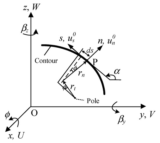
Figure 1. Schematic of the reference coordinate frames.

2.2. Laminate Constitutive Relations

The classical lamination plate theory (CLPT) [31] is used to relate the stress resultants and couples with the strains and curvatures for the shell wall of the section as given by,

$$\begin{array}{l}\left[\begin{array}{c}N\\ M\end{array}\right]=\left[\begin{array}{cc}A& B\\ B& D\end{array}\right]\left[\begin{array}{c}{ϵ}_0\\ \kappa \end{array}\right]\\ Q=kA\gamma \end{array}$$

(9)

where $N, Q, \mathrm{and} M$ are the stress resultants and couples of the laminate, and $A, B, \mathrm{and} D$ are the laminate stiffness matrices for the extension, extension-bending coupling, and bending, and k $(=5/6)$ the shear correction coefficient, respectively [16]. Following Jung et al. [16], it is assumed that the hoop stress resultant $N_{ss}$ and the transverse shear resultant $N_{sn}$ are negligibly small. While shifting the reactive components of shell stress resultants and couples such as (N_xs, M_ss, N_xn) into the right-hand side of the equation, one can express the shell constitutive relations in a semi-inverted form as:

$$\begin{array}{l}\left[\begin{array}{c}{p}_a\\ {ϵ}_r\end{array}\right]=\left[\begin{array}{cc}{C}_{aa}& C_{ar}\\ -C_{ar}^{\mathrm{T}}& C_{rr}\end{array}\right]\left[\begin{array}{c}{ϵ}_a\\ p_r\end{array}\right]\\ {\gamma }_{xn}=C_{xn}{N}_{xn}\end{array}$$

(10)

with

$$\begin{array}{l}{p}_a={\left[\begin{array}{ccc}{N}_{xx}& M_{xx}& M_{xs}\end{array}\right]}^{\mathrm{T}},\hspace{1em}\hspace{1em}{p}_r={\left[\begin{array}{cc}{N}_{xs}& M_{ss}\end{array}\right]}^{\mathrm{T}}\\ {ϵ}_a={\left[\begin{array}{ccc}{ϵ}_{xx}^0& {\kappa }_{xx}& {\kappa }_{xs}\end{array}\right]}^{\mathrm{T}},\hspace{1em}\hspace{1em}\hspace{1em} {ϵ}_r={\left[\begin{array}{cc}{\gamma }_{xs}^0& {\kappa }_{ss}\end{array}\right]}^{\mathrm{T}}\end{array}$$

(11)

where the subscripts a and r denote the active and reactive components, respectively [16,26,27,28]. The elements of the matrices $C_{aa}, C_{ar}, C_{rr}$ and $C_{xn}$ are found in Appendix A Equation (A1). Using the definition of shear strains, the active strains ${\epsilon }_a$ are expressed as follows:

$${\epsilon }_a=B_q{q}_b+{\omega }_{,x}$$

(12)

where $q_b={\left[\begin{array}{ccccc}{U}_{,x}& {\varphi }_{,x}& {\beta }_{y,x}& {\beta }_{z,x}& {\varphi }_{,xx}\end{array}\right]}^{\mathrm{T}}$ are the generalized strains of the beam, and the matrix B_q is given by

$$B_q=\left[\begin{array}{ccccc}1& 0& z& -y& {\omega }_x^{\varphi }\\ 0& 0& -y_{,s}& -z_{,s}& r_t\\ 0& 2& 0& 0& 0\end{array}\right]$$

(13)

where ${\omega }_x^{\varphi }$ is the out-of-plane warping function (unknown) under a unit twist of the cross-section. Equation (12) will be frequently recalled in the subsequent sections. It should be mentioned that only the sectional out-of-plane warping is survived due to the zero hoop stress resultant assumption ($N_{ss}=0$), and thereby the in-plane warpings are dropped out from the warping deformation arrays in $\omega$. It can be shown that the out-of-plane warping ${\omega }_x$ is found by combining the definition of the shear strain ${\gamma }_{xs}^0$ in Equations (5) and (1) as:

$${\omega }_x={\displaystyle {\int }_{s_0}^s{\gamma }_{xs}^{0}ds}-{\displaystyle {\int }_{s_0}^s{r}_{n}ds }{\varphi }_{,x}$$

(14)

The out-of-plane warping function ${\omega }_x$ is not given a priori and obtained rigorously from the derivation. Inserting the constitutive relations of ${\gamma }_{xs}^0$ into Equation (14), the out-of-plane warping deformation is obtained as:

$${\omega }_x={\omega }_q{q}_b+{\omega }_{qx}{q}_{b,x}$$

(15)

where ${\omega }_q, {\omega }_{qx}$ are the row vectors that contain the corresponding out-of-plane warping function to each entry in $q_b, q_{b,x}$ which will be determined later in the following section. It is noted that the sectional warpings are not only functions of the geometries but also the material distributions along the contour of the cross-section.

2.3. Governing Equations

The governing equations of the shell wall of the cross-section are found using a mixed variational theorem which is stated as [28]:

$$\delta \Pi =\delta U-\delta W=0$$

(16)

where the virtual strain energy per unit length, δU, and the external virtual work done over the cross-sectional area A per unit length, δW, are respectively given by [26]

$$\begin{array}{l}\delta U={\int }_C[\underset{¯}{\delta {ϵ}_a^{\mathrm{T}}{p}_a}+\delta {\left({ϵ}_r^k\right)}^{\mathrm{T}}{p}_r+\delta p_r^{\mathrm{T}}({ϵ}_r^k-{ϵ}_r)+\delta Q^{\mathrm{T}}\gamma ]ds\\ \delta W={({\int }_A\delta u_c^{\mathrm{T}}\mathbf{t}dA)}_{,x}\end{array}$$

(17)

where C is the length of the sectional contour, ${ϵ}_r^k$ is the kinematically defined reactive strains, and $t={\left[\begin{array}{ccc}{\sigma }_{xn}& {\sigma }_{xs}& {\sigma }_{xx}\end{array}\right]}^{\mathrm{T}}$ is the surface traction distributed over the cross-section. It can be shown that the variational statement of Equation (16) leads to a set of Euler-Lagrange equations followed by

$$\begin{array}{l}{N}_{xx,x}+N_{xs,s}=0\\ N_{ss,s}+N_{sn}/a+N_{xs,x}=0\\ N_{sn,s}-N_{ss}/a+N_{xn,x}=0\\ M_{xs,s}-N_{xn}+M_{xx,x}=0\\ M_{ss,s}-N_{sn}+M_{xs,x}=0\end{array}$$

(18)

along with the constraint conditions for the reactive strain and curvature components. The compatibility conditions set for the reactive strains ${ϵ}_r^{}$ are satisfied in a weak sense, while $\delta p_r^{}$ acting as the Lagrange multiplier to enforce the constraint conditions. While performing the integration by parts operation of Equation (18) leads to the following relations for the reactive shell stress resultants and couples $p_r^{\mathrm{T}}=\left[\begin{array}{cc}{N}_{xs}& M_{ss}\end{array}\right]$ as:

$$p_r=B_p{p}_r^0-p_r^b$$

(19)

with

$$\begin{array}{l}{p}_r^0={\left[\begin{array}{cccc}{N}_{xs}^0& M_{ss}^0& N_y^0& N_z^0\end{array}\right]}^{\mathrm{T}}, B_p=\left[\begin{array}{cccc}1& 0& 0& 0\\ 0& 1& z& -y\end{array}\right]\\ p_r^b=\left[\begin{array}{c}{\displaystyle {\int }_{s_0}^s{N}_{xx,x}ds}\\ {\displaystyle {\int }_{s_0}^s\left(2M_{xs,x}+N_{xs,x}{r}_n\right)ds}\end{array}\right]=S_r{q}_{b,x}\end{array}$$

(20)

where $p_r^0$ is the unknown constant of integration defined for each cell of closed cross-sections, $p_r^b$ is the vector that contains the shear flow resultant and hoop moment which vary along the cross-sectional contours, and $S_r$ is the corresponding branch flows vector, respectively. Equation (19) is inserted into $\delta p_r^{\mathrm{T}}$ in Equation (17) to have the continuity conditions for the reactive strains:

$${\displaystyle \oint B_p^{\mathrm{T}}{ϵ}_{r}ds}=A_s{q}_b$$

(21)

with $A_s$ given by

$$A_s=\left[\begin{array}{ccccc}0& {\displaystyle \oint r_{n}ds}& 0& 0& 0\\ 0& 0& 0& 0& 0\\ 0& 0& 0& 0& 0\\ 0& 0& 0& 0& 0\end{array}\right]$$

(22)

where the symbol ${\displaystyle \oint }$ denotes a closed-loop integral over the contour of the cross-section. It is remarked that there exist four sets of constraint equations for each cell of closed, multi-cell sections, similar to the cases of [16,23,26]. Inserting Equations (10) and (12) into (21), one obtains the constraint conditions expressed in a form as:

$$p_r^0=C_1{q}_b+C_2{q}_{b,x}$$

(23)

where $C_1, C_2$ are given as closed-loop integrals that represent the material distributions and sectional warpings along the contour of the shell wall. Inserting Equations (23) into (19), one can find the reactive stress resultant vector $p_r$ as:

$$\begin{array}{ll}{p}_r& =B_p{C}_1{q}_b+(B_p{C}_2-S_r)q_{b,x}\\ & =f{q}_b+g{q}_{b,x}\end{array}$$

(24)

where $f$ indicates the circuit shear flows and hoop moments of a closed cell of the cross-section with respect to the generalized beam strains, and $g$ is the resultant shear flows and hoop moments distributed along the sectional contour. The second part of Equation (24) is related with the transverse shear couplings in the Timoshenko-like beam which is neglected with the Euler–Bernoulli assumption. Having obtained the reactive stress resultant vector $p_r$, the shell transverse shear resultant N_xn can be expressed using the fourth equilibrium equations of Equation (18) along with Equation (10) as

$$N_{xn}=h{q}_b+m{q}_{b,x}$$

(25)

where $h$ and $m$ are defined similar to $f$ and $g$ in Equation (24), respectively. The effects of the transverse shear resultant N_xn should be negligible on the global beam behavior, and these have been neglected in most beam theories in the literature. Nevertheless, they are kept for more consistency and completeness in the present beam formulation.

Using Equations (7), (10), (24) and (25), the active part (singly underlined term) of the strain energy variation in Equation (16) leads to the cross-sectional stress resultants $F_b={\left[\begin{array}{ccccc}{F}_x& M_x& M_y& M_z& M_{\omega }\end{array}\right]}^{\mathrm{T}}$ expressed in terms of the generalized beam strains and their derivatives as:

$$F_b=K_{bb}{q}_b+K_{bv}{q}_{b,x}$$

(26)

where $K_{bb}$ is the (5 × 5) cross-sectional stiffness matrix that represents the beam in the Euler–Bernoulli–Vlasov level, and $K_{bv}$ represents a coupling between $F_b$ and $q_{b,x}$. The relationships between $q_b$ and the transverse shear forces $F_s$ on the cross-section are yet to be determined. The transverse shear forces affect $F_b$, resulting in the variations of the shell stress resultants and generalized strains with respect to x. The relations are obtained under a pure shear condition [27]. When the higher-order terms ($q_{b,xx}$) are neglected, the differentiation of Equation (26) by x gives

$$F_{b,x}=K_{bb}{q}_{b,x}$$

(27)

Considering the equilibrium of forces and moments of the beam in the transverse directions, one obtains the following relations

$$F_{b,x}=T_b F_s$$

(28)

with

$$T_b=\left[\begin{array}{ccc}0& 0& 0\\ 0& 0& 0\\ 0& 1& 0\\ -1& 0& 0\\ 0& 0& -1\end{array}\right],\hspace{1em}\hspace{1em}{F}_s=\left[\begin{array}{c}{F}_y\\ F_z\\ T_{\omega }\end{array}\right]$$

(29)

where $T_{\omega }$ ($T_{\omega }=-M_{\omega ,x}$) is the warping torque [2,32]. It is remarked that only the transverse shear forces remain as the independent variables since the Vlasov torsion $T_{\omega }$ is combined with the St. Venant torsion $T_{SV}$ to form the complete torsion equation: $M_x=T_{SV}+T_{\omega }$ [32]. Equating Equations (27) and (28) yields the relations between $q_{b,x}$ and $F_s$. Inserting this relation into Equations (26) yields the following equation:

$$F_b=K_{bb}{q}_b+K_{bs}{F}_s$$

(30)

with the relations $K_{bs}=K_{bv}{S}_{bb}{T}_b$ and $S_{bb}=K_{bb}^{-1}$, respectively. The pure shear condition is introduced to relate $q_b$ and $F_s$ with a null vector for $F_b$,

$$q_b=-S_{bb}{K}_{bs}{F}_s=S_{bs}{F}_s$$

(31)

A linear superposition for the bending and shear contributions from Equations (30) and (31) leads to the generalized beam strains $q_b$ expressed in terms of the generalized beam forces as:

$$q_b=S_{bb}{F}_b+S_{bs}{F}_s$$

(32)

The beam cross-sectional stiffness constants taking into account the effects of the transverse shear of the section and warping inhibition can now be determined. Using Equations (10), (12), (15), (24), and (25), one obtains the variation of strain energy in the following form:

$$\delta U=\delta {\left[\begin{array}{c}{q}_b\\ F_s\end{array}\right]}^{\mathrm{T}}{\displaystyle {\int }_C\left[\begin{array}{cc}{K}_{bb}& K_{bs}\\ K_{bs}^{\mathrm{T}}& K_{ss}\end{array}\right]}ds\left[\begin{array}{c}{q}_b\\ F_s\end{array}\right]$$

(33)

Using the relationship between $q_b$ and $F_s$ given in Equation (32), the strain energy variation in Equation (33) is transformed as:

$$\delta U=\delta {\left[\begin{array}{c}{F}_b\\ F_s\end{array}\right]}^{\mathrm{T}}{\overline{S}}_{7\times 7}\left[\begin{array}{c}{F}_b\\ F_s\end{array}\right]$$

(34)

where ${\overline{S}}_{7\times 7}$ is a (7 × 7) flexibility matrix given by

$${\overline{S}}_{7\times 7}={\left[\begin{array}{cc}{S}_{bb}& S_{bs}\\ 0& I_{2\times 2}\end{array}\right]}^{\mathrm{T}}\left[\begin{array}{cc}{K}_{bb}& K_{bv}\\ K_{bv}^{\mathrm{T}}& K_{vv}\end{array}\right]\left[\begin{array}{cc}{S}_{bb}& S_{bs}\\ 0& I_{2\times 2}\end{array}\right]$$

(35)

where $I_{2\times 2}$ is a (2 × 2) identity matrix. An inversion of the flexibility matrix yields the (7 × 7) stiffness matrix: ${\overline{K}}_{7\times 7}={\overline{S}}_{7\times 7}^{-1}$. The elements in ${\overline{K}}_{7\times 7}$ are properly rearranged so that the beam force–displacement relations of the cross-section are expressed in a convenient form:

$$F=K_{7\times 7} q$$

(36)

where

$$F={\left[\begin{array}{ccccccc}{F}_x& F_y& F_z& M_x& M_y& M_z& M_{\omega }\end{array}\right]}^{\mathrm{T}}$$

(37)

The beam generalized strains $q$ are defined previously in Equation (8b). The (7 × 7) stiffness constants K_ij describe the beam in a Timoshenko-Vlasov level while incorporating the effects of elastic couplings and shell wall thickness of composite beams. It should be noted that the transverse shear couplings essentially affect the elements of $K_{bb}$ so that the (7 × 7) stiffness constants associated with the extension, bending, torsion, and their coupled entities become substantially modified.

2.4. Recovery Relations

The stresses and strains over the shell wall thickness can be recovered through an inverse-procedure of obtaining the stiffness matrix $K_{7\times 7}$. Once the (7 × 7) stiffness constants are determined, the cross-sectional stress resultants $F$ are used to find $q_b$ via Equation (32). $q_b$ and $F_s$ are then used to evaluate the sectional warping (Equation (15)) and the reactive stress resultants $p_r$ (Equation (24)), which in turn gives the active strains ${ϵ}_a$ (Equation (12)). The reactive strains ${ϵ}_r$ are also recovered from Equation (10). With ${ϵ}_a$ and ${ϵ}_r$ are evaluated, the hoop strain ${ϵ}_{ss}^0$ which has been omitted by the zero-hoop stress flow assumption ($N_{ss}=0$) can be recovered using the laminate constitutive relations (Equation (9)) given by:

$${ϵ}_{ss}^0=-\left(A_{12}{ϵ}_{xx}^0+A_{26}{\gamma }_{xs}^0+B_{12}{\kappa }_{xx}+B_{22}{\kappa }_{ss}+B_{26}{\kappa }_{xs}\right)/A_{22}$$

(38)

where A_ij and B_ij (i, j = 1, 2, 6) are the laminate stiffness components defined in Equation (9). It is noted that the above ${ϵ}_{ss}^0$ is constructed from the constitutive relations (not from the kinematics). The recovered strains and curvatures at the midplane are then used to evaluate the (layer-wise) off-axis strains ${ϵ}_{\mathrm{off}}={\left[\begin{array}{ccc}{ϵ}_{xx}& {ϵ}_{ss}& {\gamma }_{xs}\end{array}\right]}^{\mathrm{T}}$ at any location of the shell wall with an offset n along the thickness direction as:

$${ϵ}_{\mathrm{off}}={ϵ}_0+n\kappa$$

(39)

where ${ϵ}_0$ denotes the shell strain measures at the midplane. The off-axis stresses ${\sigma }_{\mathrm{off}}={\left[\begin{array}{ccc}{\sigma }_{xx}& {\sigma }_{ss}& {\sigma }_{xs}\end{array}\right]}^{\mathrm{T}}$ are then evaluated using the stress–strain relations:

$${\sigma }_{\mathrm{off}}=\overline{Q}{ϵ}_{\mathrm{off}}$$

(40)

where $\overline{Q}$ is the off-axis lamina stiffness matrix [31]. Further recovery analysis is performed for on-axis stresses and strains using transformational relations given in [31]. It should be mentioned that the overall procedure to obtain the field variables, such as stresses and strains, are purely analytical, in the sense that all the cross-sectional stiffness constants (including sectional warpings) are obtained using a series of analytical integrations, which does not require interior domain discretizations, heavy numerical factorizations, and/or eigenvalue analyses through the entire derivation stage.

3. Numerical Examples

Numerical simulations are conducted to verify the current mixed beam formulation while demonstrating the strength and the accuracy of the proposed methodology. The examples include anisotropic rectangular strip section beam, four-layered laminated composite beam, and single-cell box section beam with circumferentially asymmetric (CAS) layup.

3.1. Anisotropic Rectangular Strip Beam

The first example is a composite thin rectangular strip section beam which has been studied by Yu and Hodges [24]. The strip is composed of a symmetric layup (bending-torsion coupling) with the dimension of the width b and the thickness h. In [24], the generalized expressions for (4 × 4) sectional stiffness constants are obtained using VAM based on the CLPT. Though their variational-asymptotic expansion has been limited by Euler–Bernoulli level, the symbolic expressions of the stiffness constants derived for an isotropic beam and the predicted values obtained for the composite strip beam are used as the reference for the cross-validation of the present results. For the composite strip beam, the non-zero stiffness constants in a Timoshenko-Vlasov level are obtained in symbolic form as:

$$\begin{gathered} K_{11}=b\left\{A_{11}^{\prime }-\frac{{\left(A_{16}^{\prime }\right)}^2}{A_{66}^{\prime }}+\underset{\_}{\frac{5{\left(A_{16}^{\prime }\right)}^2}{6A_{66}^{\prime }}}-\underset{\_}{\underset{\_}{\frac{\frac{5}{36}{\left(\frac{{\left(A_{16}^{\prime }\right)}^2}{A_{66}^{\prime }}\right)}^2}{A_{11}^{\prime }-\frac{5}{6}\frac{{\left(A_{16}^{\prime }\right)}^2}{A_{66}^{\prime }}}}}\right\} \\ {K}_{12}=-b\left\{\underset{\_}{\frac{5}{6}{A}_{16}^{\prime }}-\underset{\_}{\underset{\_}{\frac{\frac{5}{36}\frac{{\left(A_{16}^{\prime }\right)}^3}{A_{66}^{\prime }}}{A_{11}^{\prime }-\frac{5}{6}\frac{{\left(A_{16}^{\prime }\right)}^2}{A_{66}^{\prime }}}}}\right\}, K_{22}=b\left\{\underset{\_}{\frac{5}{6}{A}_{66}^{\prime }}-\underset{\_}{\underset{\_}{\frac{\frac{5}{36}{\left(A_{16}^{\prime }\right)}^2}{A_{11}^{\prime }-\frac{5}{6}\frac{{\left(A_{16}^{\prime }\right)}^2}{A_{66}^{\prime }}}}}\right\} \\ {K}_{33}=\frac{48b{\left[{\left(D_{16}^{\prime }-\frac{D_{12}^{\prime }{D}_{26}^{\prime }}{D_{22}^{\prime }}\right)}^2-\left(D_{11}^{\prime }-\frac{{(D_{12}^{\prime })}^2}{D_{22}^{\prime }}\right)\left(D_{66}^{\prime }-\frac{{(D_{26}^{\prime })}^2}{D_{22}^{\prime }}\right)\right]}^2}{b^2\left(D_{11}^{\prime }-\frac{{(D_{12}^{\prime })}^2}{D_{22}^{\prime }}\right){\left(D_{16}^{\prime }-\frac{D_{12}^{\prime }{D}_{26}^{\prime }}{D_{22}^{\prime }}\right)}^2+12C_{xn}{\left[3{\left(D_{16}^{\prime }-\frac{D_{12}^{\prime }{D}_{26}^{\prime }}{D_{22}^{\prime }}\right)}^2-2\left(D_{11}^{\prime }-\frac{{(D_{12}^{\prime })}^2}{D_{22}^{\prime }}\right)\left(D_{66}^{\prime }-\frac{{(D_{26}^{\prime })}^2}{D_{22}^{\prime }}\right)\right]}^2} \\ {K}_{44}=4b\left(D_{66}^{\prime }-\frac{{(D_{26}^{\prime })}^2}{D_{22}^{\prime }}\right), K_{45}=2b\left(D_{16}^{\prime }-\frac{D_{12}^{\prime }{D}_{26}^{\prime }}{D_{22}^{\prime }}\right), K_{55}=b\left(D_{11}^{\prime }-\frac{{(D_{12}^{\prime })}^2}{D_{22}^{\prime }}\right)K_{66}=\frac{b^3}{12}\left(A_{11}^{\prime }-\frac{{\left(A_{16}^{\prime }\right)}^2}{A_{66}^{\prime }}\right), K_{77}=\frac{b^3}{12}\left(D_{11}^{\prime }-\frac{{(D_{12}^{\prime })}^2}{D_{22}^{\prime }}\right) \end{gathered}$$

(41)

where $K_{\mathrm{ij}}$ denotes the respective entities of the stiffness matrix of $K_{7\times 7}$ given in Equation (36). The off-diagonal elements $K_{12}$ and $K_{45}$ are the extension-shear and bending-torsion couplings, respectively, which are characterized for composite strip beams. The underlined terms are responsible for the shear deformation of the cross-section in x-y plane. The terms with single underline are due to the elastic couplings between the extension and shear while the terms with double underlines are due to the sectional warpings ${\omega }_x$ related with the shear deformation. All the stiffness constants are derived in closed form which include the effects of the shell wall thickness, the transverse shear over both the shell wall and the beam, and the sectional warpings due to the couplings. It is noted that, as compared with the results of [24], the (4 × 4) stiffness coefficients expressed in symbolic form (isotropic beam) and numerical results (up to six digits) obtained for the composite beam remain identical with the present predictions (not shown explicitly), which confirms the soundness of the present mixed beam formulation.

3.2. Four-Layered Laminated Composite Beam

The next example is considered to illustrate the recovery analysis capability. A four-layered laminated composite beam employed in Liu and Yu [33] is considered for this purpose. Figure 2 shows the schematic of the beam with one end fixed and the other end subjected to a tip axial force (F_x = 10 kN). The beam is 1 m long with a width and height of 0.18 m and 0.04 m, respectively. The section consists of four layers having [90/0/90/0], which induces elastic coupling between extension and bending. The mechanical material properties are [33]: E₁ = 110.5 GPa, E₂ = E₃ = 13.64 GPa, G₁₂ = 3.92 GPa, G₁₃ = G₂₃ = 3.26 GPa, and ν₁₂ = ν₁₃ = 0.329.

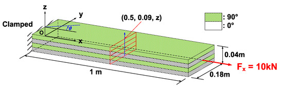
Figure 2. Schematic of the four-layer laminated beam.

In order to validate the current analysis, a detailed 3D, FE structural analysis is carried out using the commercial software MSC.NASTRAN (version: 2021.1, MSC software, Irvine, CA, United States, https://www.mscsoftware.com/product/msc-nastran (access date: 28 July 2022)). The beam is discretized using the 20-noded solid element (CHEXA) having 8 finite elements through the thickness, 36 elements along the width, and 200 elements along the beam length, leading to 57,600 in total. A RBE2 element is used to apply the axial load at the free tip. The predicted stresses through the thickness direction at the center of the beam, as indicated in Figure 2, are compared against the results by Liu and Yu [33] and the 3D solid FE analysis. Figure 3 shows the comparison between the three sets of results obtained respectively for the normal stresses (${\sigma }_{xx}, {\sigma }_{yy}$) distributed through the thickness. It is observed that the present results are in excellent agreements with the detailed 3D FE results and the other beam prediction. It is emphasized that, as can be seen in Figure 3b, the in-plane normal stress ${\sigma }_{yy}$ along the shell wall can also be recovered using Equation (40), even though the deformation along the contour is kinematically suppressed due to the zero-hoop stress flow assumption.

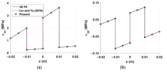
Figure 3. Comparison of predicted normal stresses through the thickness between 3D FE, Liu and Yu (2016) [33] and the present: (a) axial stress; (b) transverse stress.

3.3. Single-Cell Composite Box Beam with CAS Layup

The third example is a thin-walled, single-cell box-section beam with CAS layup, which has been exploited by many researchers for the validation works [34,35,36]. Figure 4 shows the geometry and the ply layup which induce couplings between bending-torsion and extension-shear motions. The outer dimensions of the box section are: b = 24.206 mm, h = 13.640 mm, with the thickness of an individual layer t = 0.127 mm. The effective length of the cantilevered beam is 762 mm. The positive directions of the local curvilinear coordinates at each wall are indicated in Figure 4. The mechanical material properties are given as [36]: E₁ = 141.96 GPa, E₂ = E₃ = 9.79 Gpa, G₁₂ = G₁₃ = 6.00 Gpa, G₂₃ = 4.80 Gpa, ν₁₂ = ν₁₃ = 0.42.

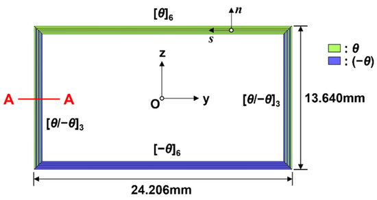
Figure 4. Geometry and ply layup structure of the composite single-cell box section.

Table 1 shows the comparison of non-zero stiffness constants predicted between the present analysis and the other references [34,35,36] for the box-section beam when the ply orientation angle θ is set to 15 deg. The NABSA is a code name for detailed FE beam model constructed based on the work of Giavotto et al. [5], and the stiffness results are taken from Popescu and Hodges [34]. The work of Krenk and Couturier [35] uses 3D Fes to compute the stiffness parameters using a complementary form of the strain energy. In Dhadwal and Jung [36], 2D FE-based section analysis method is developed to compute (6 × 6) stiffness constants where 3D warpings and stress fields over the cross-sectional nodes are solved simultaneously. The comparison results indicate good agreements between the different sets of predictions. The maximum error of the present computation is less than 1.9%, as compared with the more involved, FE-based cross-sectional analysis predictions, which proves the validity of the present mixed beam approach.

Table 1. Comparison of non-zero stiffness constants of single-cell composite box section.

Stiffness	NABSA [34]	Krenk et al. (2017) [35] (%) 1	Dhadwal et al. (2019) [36] (%) 1	Present (%) 1
K11 (N)	6.0938 × 106	6.1100 × 106 (0.27)	6.1200 × 106 (0.43)	6.1124 × 106 (0.31)
K12 (N)	8.1843 × 105	8.1900 × 105 (0.07)	8.1600 × 105 (−0.30)	8.1413 × 105 (−0.53)
K22 (N)	3.9320 × 105	3.9400 × 105 (0.20)	3.9500 × 105 (0.46)	3.8774 × 105 (−1.39)
K33 (N)	1.7570 × 105	1.7600 × 105 (0.17)	1.7700 × 105 (0.74)	1.7247 × 105 (−1.83)
K44 (N-m2)	4.9645 × 101	4.9800 × 101 (0.31)	5.0000 × 101 (0.71)	4.9093 × 101 (−1.11)
K45 (N-m2)	−5.1654 × 101	−5.1800 × 101 (0.28)	−5.1500 × 101 (−0.30)	−5.1503 × 101 (−0.29)
K55 (N-m2)	1.7448 × 102	1.7500 × 102 (0.30)	1.7500 × 102 (0.30)	1.7439 × 102 (−0.05)
K66 (N-m2)	4.1036 × 102	4.1000 × 102 (−0.09)	4.1200 × 102 (0.40)	4.0844 × 102 (−0.47)

¹ Percentage differences are evaluated with respect to NABSA values as: (Analysis-NABSA)/NABSA × 100.

The sectional warping deformation modes (continuous lines) associated with the six fundamental modes of extension, shear, torsion and bending are presented in Figure 5 along with their corresponding undeformed modes (dashed lines). As is indicated in the plots, all the warping deformations are influenced by the couplings between the extension-shear and bending-torsion motions. In Figure 6, the predicted stresses of the composite box beam subjected to a unit tip shear load (4.448 N) are compared against the ones of Dhadwal and Jung [36] and 3D FE analysis using the MSC.NASTRAN. The 3D FE model consists of 20-noded 1,152,000 CHEXA solid elements, along with a RBE2 element installed at the tip for the load application. Figure 6 presents the layer-wise distribution of stresses obtained along the A-A line of the left wall of the box section (see Figure 4). The in-plane normal stress ${\sigma }_{ss}$ is recovered as well as the other shell stress components (${\sigma }_{xx}, {\sigma }_{xs}$). It is observed that the present predictions capture the general trends of the linear variation over each layer of the box section, with the amplitudes agreed well with those of the detailed FE-based method and 3D FE analysis. The comparison demonstrates again the validity of the present work for the stress recovery analysis capability of closed cross-sections. It should be noted that the present predictions are resulted from purely analytical treatments of the sectional integrals without resorting to any mesh discretization over the cross-section. No convergence check is needed as well, such as the case with the FE-based approaches, which greatly saves the computation cost.

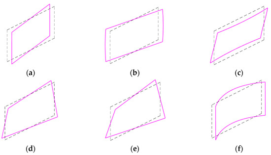
Figure 5. Out-of-plane warping modes under unit loads: (a) F_x; (b) F_y; (c) F_z; (d) M_x; (e) M_y; (f) M_z.

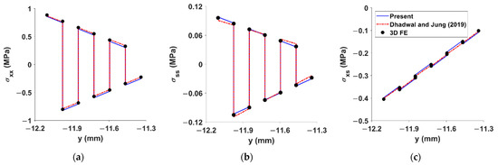
Figure 6. Comparison of the layer-wise stress distributions at the left wall between the present, Dhadwal and Jung (2019) [36] and 3D FE: (a) axial stress; (b) hoop stress; (c) tangential stress.

4. Concluding Remarks

In this study, a variationally consistent, thin-walled composite beam model was developed combining the mixed beam theory and the generalized beam formulation. Starting from the shell theory, the Euler–Lagrange equations and the constraint conditions of the shell wall of the beam were obtained correctly as the part of the analysis. In order to facilitate the beam analysis, a zero-hoop stress flow assumption was retained for the sectional wall. The effects of the shell wall thickness and the out-of-plane warpings derived from the constitutive relations were incorporated in the theory, leading to the (7 × 7) stiffness constants equivalent to the level of Timoshenko-Vlasov beam. Three different, elastically coupled composite beams were tested to show the validity of the present analysis. First, symbolic expressions were derived explicitly for (7 × 7) stiffness constants of an anisotropic strip beam, identifying each of the contributing terms due to the couplings. Next, the cross-sectional warping deformation modes associated with the loads were identified while capturing the coupling behavior of the beam motions. All the stress fields including the in-plane stress were recovered and compared with 3D FE and other detailed cross-sectional analysis results, resulting in an excellent correlation between the predictions. Finally, the comparison of the stiffness constants for composite box section demonstrated a deviation less than 1.9%, against up-to-date FE-based methods. Given no mesh discretization nor heavy numerical factorization was involved in obtaining the warping and stiffness constants, the present work demonstrated excellent prediction capability which could be exploited further for an optimum structural design of composite helicopter blades and wind turbine blades.

References

- Hodges, D.H. Review of composite rotor blade modeling. AIAA J. 1990, 28, 561–565. [Google Scholar] [CrossRef]
- Jung, S.N.; Nagaraj, V.T.; Chopra, I. Assessment of composite rotor blade modeling techniques. J. Am. Helicopter Soc. 1999, 44, 188–205. [Google Scholar] [CrossRef]
- Hodges, D.H. Nonlinear Composite Beam Theory; American Institute of Aeronautics and Astronautics: Reston, VA, USA, 2006. [Google Scholar]
- Berdichevskii, V.L. On the energy of an elastic rod. J. Appl. Math. Mech. 1982, 45, 518–529. [Google Scholar] [CrossRef]
- Giavotto, V.; Borri, M.; Mantegazza, P.; Ghiringhelli, G.; Carmaschi, V.; Maffioli, G.; Mussi, F. Anisotropic beam theory and applications. Comput. Struct. 1983, 16, 403–413. [Google Scholar] [CrossRef]
- Morandini, M.; Chierichetti, M.; Mantegazza, P. Characteristic behavior of prismatic anisotropic beam via generalized eigenvectors. Int. J. Solids Struct. 2010, 47, 1327–1337. [Google Scholar] [CrossRef]
- Yu, W.; Hodges, D.H.; Ho, J.C. Variational asymptotic beam sectional analysis—An updated version. Int. J. Eng. Sci. 2012, 59, 40–64. [Google Scholar] [CrossRef]
- Han, S.; Bauchau, O.A. Nonlinear three-dimensional beam theory for flexible multibody dynamics. Multibody Syst. Dyn. 2015, 34, 211–242. [Google Scholar] [CrossRef]
- Dhadwal, M.K.; Jung, S.N. Multifield variational sectional analysis for accurate stress computation of multilayered composite beams. AIAA J. 2019, 57, 1702–1714. [Google Scholar] [CrossRef]
- Carrera, E.; Giunta, G. Refined beam theories based on a unified formulation. Int. J. Appl. Mech. 2010, 2, 117–143. [Google Scholar] [CrossRef]
- Carrera, E.; de Miguel, A.; Pagani, A. Hierarchical theories of structures based on Legendre polynomial expansions with finite element applications. Int. J. Mech. Sci. 2017, 120, 286–300. [Google Scholar] [CrossRef]
- Heyliger, P.R. Elasticity alternatives to generalized Vlasov and Timoshenko models for composite beams. Compos. Struct. 2016, 145, 80–88. [Google Scholar] [CrossRef]
- Yu, W.; Hodges, D.H. Elasticity solutions versus asymptotic sectional analysis of homogeneous, isotropic, prismatic beams. J. Appl. Mech. 2004, 71, 15–23. [Google Scholar] [CrossRef]
- Ho, J.C. Shear Stiffness of Homogeneous, Orthotropic, Prismatic Beams. AIAA J. 2017, 55, 4357–4363. [Google Scholar] [CrossRef]
- Smith, E.C.; Chopra, I. Formulation and evaluation of an analytical model for composite box beams. J. Am. Helicopter Soc. 1991, 36, 23–35. [Google Scholar] [CrossRef]
- Jung, S.N.; Nagaraj, V.T.; Chopra, I. Refined structural model for thin- and thick-walled composite rotor blades. AIAA J. 2002, 40, 105–116. [Google Scholar] [CrossRef]
- Librescu, L.; Song, O. Thin-Walled Composite Beams: Theory and Application; Springer: Berlin/Heidelberg, Germany, 2006. [Google Scholar]
- Zhang, C.; Wang, S. Structural mechanical modeling of thin-walled closed-section composite beams, Part 1: Single-cell cross section. Compos. Struct. 2014, 113, 12–22. [Google Scholar] [CrossRef]
- Vo, T.P.; Lee, J. Flexural–torsional behavior of thin-walled closed-section composite box beams. Eng. Struct. 2007, 29, 1774–1782. [Google Scholar] [CrossRef][Green Version]
- Vieira, R.; Virtuoso, F.; Pereira, E. A higher order model for thin-walled structures with deformable cross-sections. Int. J. Solids Struct. 2014, 51, 575–598. [Google Scholar] [CrossRef]
- Han, S.; Bauchau, O.A. On the analysis of thin-walled beams based on Hamiltonian formalism. Comput. Struct. 2016, 170, 37–48. [Google Scholar] [CrossRef]
- Deo, A.; Yu, W. Thin-walled composite beam cross-sectional analysis using the mechanics of structure genome. Thin-Walled Struct. 2020, 152, 106663. [Google Scholar] [CrossRef]
- Volovoi, V.V.; Hodges, D.H. Theory of anisotropic thin-walled beams. J. Appl. Mech. 2000, 67, 453–459. [Google Scholar] [CrossRef]
- Yu, W.; Hodges, D.H. Best Strip-Beam Properties Derivable from Classical Lamination Theory. AIAA J. 2008, 46, 1719–1724. [Google Scholar] [CrossRef]
- Harursampath, D.; Harish, A.B.; Hodges, D.H. Model reduction in thin-walled open-section composite beams using variational asymptotic method. Part I: Theory. Thin-Walled Struct. 2017, 117, 356–366. [Google Scholar] [CrossRef]
- Reissner, E.; Tsai, W.T. Pure bending, stretching, and twisting of anisotropic cylindrical shells. J. Appl. Mech. 1972, 39, 148–154. [Google Scholar] [CrossRef]
- Tsai, W. On the problem of flexure of anisotropic cylindrical shells. Int. J. Solids Struct. 1973, 9, 1155–1175. [Google Scholar] [CrossRef]
- Reissner, E. On mixed variational formulations in finite elasticity. Acta Mech. 1985, 56, 117–125. [Google Scholar] [CrossRef]
- Murakami, H.; Reissner, E.; Yamakawa, J. Anisotropic beam theory with shear deformation. J. Appl. Mech. 1996, 63, 660–668. [Google Scholar] [CrossRef]
- Kraus, H. Thin Elastic Shells; Wiley: New York, NY, USA, 1967. [Google Scholar]
- Jones, R.M. Mechanics of Composite Materials, 2nd ed.; Taylor and Francis: Boca Raton, FL, USA, 1999. [Google Scholar]
- Jung, S.N.; Lee, J.Y. Closed-form analysis of thin-walled composite I-beams considering non-classical effects. Compos. Struct. 2003, 60, 9–17. [Google Scholar] [CrossRef]
- Liu, X.; Yu, W. A novel approach to analyze beam-like composite structures using mechanics of structure genome. Adv. Eng. Softw. 2016, 100, 238–251. [Google Scholar] [CrossRef]
- Popsecu, B.; Hodges, D.H. On asymptotically correct Timoshenko-like anisotropic beam theory. Int. J. Solids Struct. 2000, 37, 535–558. [Google Scholar] [CrossRef]
- Krenk, S.; Couturier, P.J. Equilibrium-based nonhomogeneous anisotropic beam element. AIAA J. 2017, 55, 2773–2782. [Google Scholar] [CrossRef]
- Dhadwal, M.K.; Jung, S.N. Generalized multifield variational formulation with interlaminar stress continuity for multilayered anisotropic beams. Compos. B Eng. 2019, 168, 476–487. [Google Scholar] [CrossRef]
Publisher’s Note: MDPI stays neutral with regard to jurisdictional claims in published maps and institutional affiliations. |
© 2022 by the authors. Licensee MDPI, Basel, Switzerland. This article is an open access article distributed under the terms and conditions of the Creative Commons Attribution (CC BY) license (https://creativecommons.org/licenses/by/4.0/).