Heat Conduction and Microconvection in Nanofluids: Comparison between Theoretical Models and Experimental Results

Abstract

A nanofluid is a suspension consisting of a uniform distribution of nanoparticles in a base fluid, generally a liquid. Nanofluid can be used as a working fluid in heat exchangers to dissipate heat in the automotive, solar, aviation, aerospace industries. There are numerous physical phenomena that affect heat conduction in nanofluids: clusters, the formation of adsorbate nanolayers, scattering of phonons at the solid–liquid interface, Brownian motion of the base fluid and thermophoresis in the nanofluids. The predominance of one physical phenomenon over another depends on various parameters, such as temperature, size and volume fraction of the nanoparticles. Therefore, it is very difficult to develop a theoretical model for estimating the effective thermal conductivity of nanofluids that considers all these phenomena and is accurate for each value of the influencing parameters. The aim of this study is to promote a way to find the conditions (temperature, volume fraction) under which certain phenomena prevail over others in order to obtain a quantitative tool for the selection of the theoretical model to be used. For this purpose, two sets (SET-I, SET-II) of experimental data were analyzed; one was obtained from the literature, and the other was obtained through experimental tests. Different theoretical models, each considering some physical phenomena and neglecting others, were used to explain the experimental results. The results of the paper show that clusters, the formation of the adsorbate nanolayer and the scattering of phonons at the solid–liquid interface are the main phenomena to be considered when φ = 1 ÷ 3%. Instead, at a temperature of 50 °C and in the volume fraction range (0.04–0.22%), microconvection prevails over other phenomena.

1. Introduction

Since the second half of the 1990s, nanoparticle fluid suspensions, commonly referred to as nanofluids, have attracted the attention of researchers due to the need to develop a heat transfer fluid with higher energy performance. The use of nanofluids has many advantages and has therefore been applied in various fields in recent years [1,2], such as in the automotive sector, in solar energy systems, in heat exchangers, in aerospace—all areas where heat dissipation plays a fundamental role and does not only include the nanofluids used to lubricate mechanical parts, which have higher viscosity, are more efficient or improve heat transfer performance in a possible application of regenerative cooling of rocket engine thrust chambers [3]. Nanofluids can thus be used to cool electronic components or as transmission fluids in solar and photovoltaic panels. The main advantage is that lower mass flow rates are required for a nanofluid, which allows the construction of smaller heat exchangers. This is a major advantage in the aerospace field where the available volume is limited. A fluid with ultrafine suspended nanoparticles will be an advanced fluid for satellite heat pipe applications because it does not require oil, is compact, has less weight and low power consumption, all of which are particularly important for space applications [4,5].

Its production is possible thanks to the advent of nanotechnologies, which were matured for this purpose during those years. One of the first studies on nanofluids dates back to 1995, to the work of Eastman and Choi [6], who analyzed the advantages of using such a fluid. In 1999, one of the first experimental papers on nanofluids was published by Lee and Choi [7], who studied the improvement in thermal conductivity of water/alumina, glycol/alumina and water/copper oxide. The authors observed a direct proportionality between the thermal conductivity and the volumetric concentration of nanoparticles (φ) for small volumetric concentrations (less than 5%). The influence of the type of base fluid and the thermal conductivity of the nanoparticles was also investigated.

Subsequent studies confirmed the effect of volumetric concentration but showed some differences between publications. For the same nanofluid and for the same volumetric concentration, different increases in thermal conductivity were demonstrated. For example, for water–alumina nanofluids with a volumetric concentration of 2% and an average particle diameter of 50 nm, Beck et al. [8] and Kokate et al. [9] found an increase in thermal conductivity of 9% in Ref. [8] and 15% in Ref. [9]. At a volumetric concentration of 3% and the same average diameter, it increased by 14% in Ref. [8] and 20% in Ref. [9].

Different results can be obtained with different types of nanoparticles. For example, in Ref. [10], the authors found an improvement in thermal conductivity between 2.1 and 3.5% with the ZnO nanofluid, while in Ref. [11], an improvement of 8.7% was obtained with 0.2% TiO₂ nanofluids.

In 2009, the International Nanofluid Property Benchmark Exercise (INPBE) experimental study [12] showed that the different results described above can be avoided by close cooperation between the institutes conducting the studies. The reason for these discrepancies is indeed the inhomogeneity of the (nominally identical) nanofluids during manufacturing. In addition, an incomplete data sheet of the particles used can lead to inaccuracies. Unfortunately, not all nanoparticle suppliers provide the same level of detail of nanoparticle fabrication. Using the method proposed in Ref. [12], it is possible to reduce the differences between measurements reported by different research groups to as little as 10%. In Ref. [12], the measurements were performed in a temperature range between 20 °C and 30 °C, and the influence of particle size on the thermal conductivity of nanofluids was not analyzed. The model used to explain the experimental data was the Nan model [13], which generalizes the Hamilton–Crosser model [14] to any particle morphology and takes into account the phenomenon of phonon scattering at the solid–liquid interface.

In Ref. [13], the authors show that the volumetric concentration of nanoparticles affects the thermal conductivity of nanofluids, and they also claim that thermal conductivity predictions are more accurate when a non-zero Kapitza resistance is considered (typically R_bd = 10⁻⁸ m² K·W⁻¹).

Other discrepancies in the scientific literature on thermal conductivity behavior can be attributed to particle size [8,9,15,16]. Indeed, some analytical models, such as that of Nan and Feng, lead to opposite predictions of thermal conductivity. Moreover, some experimental studies [8,15] show a proportional trend of thermal conductivity as a function of particle size, while other studies [9,16] show an opposite trend for the same nanofluids.

It turns out that heat conduction in nanofluids is a very complex phenomenon. In fact, there are numerous physical phenomena that affect heat conduction in nanofluids: clump formation, formation of the adsorbing nanolayer, scattering of phonons at the solid–liquid interface, Brownian motion of the base fluid and thermophoresis in the nanofluids. The physiological parameters that make these phenomena more or less evident are the size and shape of the particles, the nature of the particles and the base fluid, the temperature and the concentration of the nanoparticles. Unfortunately, there is no theoretical model that can take into account all the above physical phenomena simultaneously and predict the thermal conductivity of the nanofluid under all conditions (temperature, volume fraction of nanoparticles) [17].

Therefore, it is very useful to know and quantify the physical conditions (temperature, particle size, volumetric concentration) that make some physical phenomena more significant and others negligible. In this way, based on the physical parameters and the operating conditions, it is possible to determine the theoretical models that predict the thermal conductivity of the nanofluid with greater accuracy.

This paper presents a way to determine the conditions (temperature, particle size, nanoparticle volume fraction) under which certain phenomena prevail and to provide a quantitative tool for selecting the theoretical model to be used. For this purpose, two sets of experimental data were analyzed; one was obtained from the literature, and the other was obtained through experimental tests. Different theoretical models were used to describe the experimental data. The analysis of the data, supported by theoretical models, allowed us to determine which of these models provides a more accurate prediction of thermal conductivity.

2. Theoretical Models

Over the past decade, numerous theoretical models have been formulated to predict the thermal conductivity of nanofluids [17]. This section presents the theoretical models chosen to describe the experimental data.

2.1. Hamilton–Crosser Model

The first model presented is the Hamilton–Crosser (H-C) model. In this model [14], every particle shape can be considered. The model is an extension of Maxwell Garnett (M-G) [18,19].

The equation of the H-C model is as follows:

$$\frac{k}{k_{bf}}=\frac{k_p+\left(n-1\right)k_{bf}-\left(n-1\right)\phi \left(k_{bf}-k_p\right)}{k_p+\left(n-1\right)k_{bf}+\phi \left(k_{bf}-k_p\right)}$$

(1)

The empirical parameter n is equal to 3/Ψ, where Ψ is the sphericity, defined as the ratio between the surface area of a sphere with a volume equal to that of the particle and the surface area of the particle. When n = 3, the M-G equation is obtained. The Hamilton–Crosser model takes into account the nature of the constituents, the shape and the volumetric concentration of the nanoparticles. However, it does not take into account the effects of particle size. The advantage of the H-C model is that it provides an asymptotic limit with respect to other theoretical models (e.g., an upper limit for Nan and a lower limit for Feng).

2.2. Nan Model

The Nan model [13] is a phenomenological model, which extends the H-C model. The model considers a general morphology of “particles” (nanoparticles can have any morphology: nanotubes, nanolayers, etc.). In addition, the Nan model takes into account the phenomenon of phonon scattering at the solid–liquid interface (the Kapitza model is used to include resistance [20]). To analyze the experimental set of this paper, the case of ellipsoidal particles was considered; therefore, the formula is given for this type of particle.

$$\frac{k}{k_{bf}}=\frac{3+\phi \left[2{\beta }_{11}\left(1-L_{11}\right)+{\beta }_{33}\left(1-L_{33}\right)\right]}{3-\phi \left[2{\beta }_{11}{L}_{11}+{\beta }_{33}{L}_{33}\right]}$$

(2)

Equation (2) was used with a₁ = a₃, where a₁ and a₃ are the principal semiaxes of the particle in directions 1 and 3, respectively, and L_ii are the geometric parameters defined as follows:

$$L_{11}=L_{22}=\{\begin{array}{l}\frac{p^2}{2\left(p^2-1\right)}-\frac{p}{2{\left(p^2-1\right)}^{3/2}}{\cosh }^{-1}\left(p\right)\hspace{1em}if\hspace{0.17em}p>1\\ \frac{p^2}{2\left(p^2-1\right)}+\frac{p}{2{\left(p^2-1\right)}^{3/2}}{\cosh }^{-1}\left(p\right)\hspace{1em}if\hspace{0.17em}p<1\\ 1/3\hspace{1em}\hspace{1em}\hspace{1em}\hspace{1em}\hspace{1em}\hspace{1em}\hspace{1em}\hspace{1em}\hspace{1em}\hspace{1em} if\hspace{0.17em}p=1\end{array}$$

(3)

$$L_{33}=1-2L_{11}$$

(4)

with $p=\frac{a_3}{a_1}$ the aspect ratio

$${\beta }_{ii}=\frac{k_{ii}^c-k_{bf}}{k_{bf}+L_{ii}\left(k_{ii}^c-k_{bf}\right)}$$

(5)

$$k_{ii}^c=\frac{k_p}{1+\gamma L_{ii}{k}_p/k_{bf}}$$

(6)

and

$$\gamma =\{\begin{array}{l}\left(2+1/p\right)\alpha \hspace{1em}if\hspace{0.17em}p\ge 1\\ \left(1+2p\right)\alpha \hspace{1em}if\hspace{0.17em}p\le 1\end{array}$$

(7)

$$\alpha =\{\begin{array}{l}{a}_k/a_1\hspace{1em}if\hspace{0.17em}p\ge 1\\ a_k/a_3\hspace{1em}if\hspace{0.17em}p\le 1\end{array}$$

(8)

$$a_k=R_{bd}{k}_{bf}$$

(9)

$R_{bd}$ is the Kapitza resistance, i.e., a thermal resistance used to describe the effect of phonon scattering, which is an opposite resistance contribution to heat transfer.

The Nan model also takes into account the scattering of phonons at the interface. When R_bd = 0 m²K/W, the H-C model is obtained. It is obvious that the H-C model represents the upper limit of the Nan model, which is reached when the particle size increases.

2.3. Modified Geometric Mean

This model was developed by Warrier et al. [15] to generalize the geometric mean formula of Turian et al. [21]. The purpose of the modified geometric mean is to make explicit some of the physical phenomena included in the empirical parameter “m”. These phenomena are the deviation of the thermal conductivity of nanoparticles compared to the analogous bulk material (Matthiessen rule [16]) and the influence of temperature on the electronic thermal conductivity [22]. Ultimately, the model description can be written as follows:

$$k^m=k^m\phi +k_{bf}^m\left(1-\phi \right)\hspace{1em}-1\le m\le 1$$

(10)

m is an empirical parameter.

Applying the Matthiessen rule [9]

$$\{\begin{array}{l}\frac{k_p}{k_b}=\frac{{\lambda }_{e,p}}{{\lambda }_{e,b}}=\frac{1}{1+Kn}\hspace{1em}if\hspace{1em}Kn\le 1\\ \mathrm{Linear}\hspace{0.17em}\mathrm{interpolation}\hspace{1em}if\hspace{0.17em}1<Kn<5\\ \frac{k_p}{k_b}=\frac{{\lambda }_{e,p}}{{\lambda }_{e,b}}=\frac{1}{Kn}\hspace{1em}if\hspace{1em}Kn\ge 5\end{array}$$

(11)

$$Kn=\frac{{\lambda }_{e,b}}{d}$$

(12)

where λ_e,p and λ_e,b are, respectively, the mean free path of conduction electrons in the particle and in the bulk; Kn is the Knudsen number; k_b is the thermal conductivity of the bulk material given by the Sommerfeld model:

$$k_b\left(T\right)=\frac{n_e{\pi }^2{K}^{2}T{\lambda }_{e,b}}{3m_e{v}_f}$$

(13)

n_e is the electronic density; m_e is the electron mass; K is the Boltzmann constant; and v_f Fermi is the velocity of the conduction electrons.

It is appropriate to point out the empirical nature of this model, since it includes the empirical parameter m to describe the conductivity of the nanofluid (Equation (10)). The correct choice of m makes it possible to describe the phenomena affecting the thermal conductivity of the nanofluid. However, the parameter m depends on many other phenomena, which are not taken into account by the modified geometric mean. Therefore, the determination of “m” is not straightforward because “m” hides all the phenomena that have not been explicitly expressed. For this reason, the geometric mean model has more statistical than phenomenological significance. However, the extremes of the parameter “m” allow us to distinguish between two types of conduction:

• m = −1: the two components conduct the heat flow in series;
• m = 1: in this case, the two components conduct the heat flow in parallel.

2.4. Feng Model

The Feng model [23] assumes that the nanoparticles have a spheroidal shape. The Feng model allows us to take into account the adsorbed layer (covering the nanoparticles) and the presence of 2D lattice clusters.

The thermal conductivity of nanofluids is estimated using the following formula:

$$k=\left(1-{\phi }_e\right)k_m+{\phi }_e{k}_a$$

(14)

$$k_a=\left(1-\frac{3}{2}{\phi }_e\right)k_{bf}+\frac{3{\phi }_e{k}_{bf}}{\beta }\left[\frac{1}{\beta }ln\left(\frac{1}{1-\beta }\right)-1\right]$$

(15)

where k_a is the thermal conductivity of the cluster region of the fluid (Figure 1); ${\phi }_e=\phi \left(1+{\delta }^3\right)$ is the effective volumetric concentration (the explanation is reported below); $\delta =h/a$ is the ratio between nanolayer thickness and the original particle radius; $\beta =1-k_{bf}/k_{pe}$, $r=a$ is the particle radius; h is the nanolayer thickness;

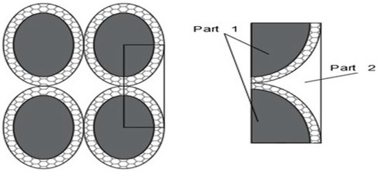
Figure 1. 2D Reticular Cluster, Feng [23].

k_m is calculated as follows:

$$k_m=\frac{k_{p\hspace{0.17em}e}+2k_{bf}+2\left(k_{p\hspace{0.17em}e}-k_{bf}\right){\left(1+\delta \right)}^3\phi }{k_{p\hspace{0.17em}e}+2k_{bf}-\left(k_{p\hspace{0.17em}e}-k_{bf}\right){\left(1+\delta \right)}^3\phi }{k}_{bf}$$

(16)

$k_{p\hspace{0.17em}e}$ is the effective thermal conductivity of the particles:

$$k_{p\hspace{0.17em}e}=\frac{\gamma \left[2\left(1-\gamma \right)+{\left(1+\delta \right)}^3\left(1+2\gamma \right)\right]}{\left(\gamma -1\right)+{\left(1+\delta \right)}^3\left(1+2\gamma \right)}{k}_p$$

(17)

$\gamma =k_{layer}/k_p$ is the ratio between nanolayer thermal conductivity and that of the particles.

The entity of the cluster in the nanofluid is quantified by the effective volumetric concentration (φ_e) (particle size plus the thickness of the layer with which they are coated). Since the effective volumetric concentration (φ_e) is significantly higher than the contribution of the nanoparticles alone, the presence of clusters and a nanolayer increases the thermal conductivity of the nanofluid.

The tendency for the cluster to form is greater as the particle size decreases. Small particles are closer together than large ones, creating a greater attractive force.

In the Feng model, particles are considered as spheres, so applying this model to particles with an elongated shape (e.g., ellipsoidal) can be considered an extension of the model. To simplify the approach, the particles are considered to be ellipsoidal. According to the method described by Feng [23], it is possible to obtain a formula similar to Equation (14). If the particle cluster is considered to be arranged ellipsoidal, as shown in Figure A1

$$k_e=\left(1-{\phi }_e^{\prime }\right)k_{hc}+{\phi }_e{k}_a^{\prime }$$

(18)

with

$$k_a^{\prime }=\left(1-\frac{3}{2}{\phi }_e^{\prime }\right)k_{bf}+3{\phi }_e^{\prime }\frac{\left(a_1+h^3\right)}{\left(a_3+h^3\right)}\cdot \frac{k_{bf}\beta \left[\left(\beta -1\right)+\beta \hspace{0.17em}ln\left(\beta \right)\right]}{{\left(\beta -1\right)}^2}$$

(19)

$$k_{hc}=k_{bf}\frac{k_{{}_{pe}}^{\prime }+\left(n-1\right)k_{bf}-\left(n-1\right){\phi }_{{}_e}^{\prime }\left(k_{bf}-k_{{}_{pe}}^{\prime }\right)}{k_{{}_{pe}}^{\prime }+\left(n-1\right)k_{bf}+{\phi }_{{}_e}^{\prime }\left(k_{bf}-k_{{}_{pe}}^{\prime }\right)}$$

(20)

$$k_{pe}^{\prime }=\frac{\left\{\left(n-1\right)\left(1-\gamma \right)+{\left(1+{\delta }_1\right)}^2\left(1+{\delta }_3\right)\left[1+\left(n-1\right)\gamma \right]\right\}\gamma }{\left(\gamma -1\right)+{\left(1+{\delta }_1\right)}^2\left(1+{\delta }_3\right)\left[1+\left(n-1\right)\gamma \right]}{k}_p$$

(21)

$${\phi }_{{}_e}^{\prime }=\phi {\left(1+{\delta }_1\right)}^2\left(1+{\delta }_3\right)$$

(22)

where ${\delta }_1=h/a_1$, ${\delta }_3=h/a_3$, $\beta =1-k_{bf}/k_{{}_{pe}}^{\prime }$ with a₁ and a₃ the principal semiaxes of the ellipsoid, with a₁ = a₂. It can be observed that Equation (18) agrees with the original Feng Equation (14) in the case of spheroidal particles (n = 3, a₁ = a₃). Appendix A details the complete demonstration, which the authors carried out for the extension of the Feng model.

2.5. Prasher Model

The Prasher model [24] takes into account the scattering of phonons (although only partially) and the presence of fractal clusters. The Prasher model predicts the thermal conductivity of the nanofluid with the following equation:

$$k=\frac{k^{\prime }+2k_{bf}+2\left(k^{\prime }-k_{bf}\right){\phi }_a}{k^{\prime }+2k_{bf}-\left(k^{\prime }-k_{bf}\right){\phi }_a}{k}_{bf}$$

(23)

where $k^{\prime }$ is the thermal conductivity of the cluster, which has a dimension equal to the radius of inertia, and φ_a is the volume fraction of the aggregates.

Nan’s modeling of backbone particles for ellipsoidal particles (with aspect ratio p = R_g/a) represents a limit of the Prasher model. A backbone is a more complicated object formed by a columnar aggregation of nanoparticles. The approximation of the backbone structure leads to a further increase in thermal conductivity. In fact, all those surfaces within the envelope of the ellipsoid where phonon scattering occurs are lost. The surface area affected by phonon scattering is considered to be smaller than it actually is.

2.6. Corcione Model

In order to take into account all the phenomena related to microconvection (Brownian motion and thermophoresis), Corcione developed his model [25], which is an empirical formula based on dimensional analysis. This model does not allow a phenomenological analysis of microconvection, but it does allow us to understand when microconvection can be neglected or not. The empirical equation established by Corcione et al. is as follows:

$$\frac{k}{k_{fb}}=1+4.4{\mathrm{Re}}_p^{0.40}{\mathrm{Pr}}_{bf}^{0.66}{\left(\frac{T}{T_{fr}}\right)}^{10}{\left(\frac{k_p}{k_{bf}}\right)}^{0.03}{\phi }^{0.66}$$

(24)

$${\mathrm{Re}}_p^{}=\frac{2{\rho }_{bf}KT}{\pi {\mu }_{bf}^2{d}_p}$$

(25)

Re is the Reynolds number of the nanoparticles; Pr is the Prandtl number of the base liquid; T is the nanofluid temperature; T_fr is the freezing point of the base liquid; k_p is the thermal conductivity of the nanoparticles; and φ is the volume fraction of the suspended nanoparticles. K is the Boltzmann constant.

3. Experimental Data Sets

The experimental data analyzed in this paper are two sets of data; the first set comes from the INPBE report [12], while the second set was obtained experimentally by the authors.

3.1. SET-1

In the original INPBE report, the data were interpreted using only the Nan model; in this paper, the same data were described using the other models described above. The data from SET-1 are measurements of the thermal conductivity of alumina nanofluids. Samples 3 and 4 are nanofluids prepared with alumina nanoparticles, while Samples 5 and 6 were prepared with alumina nanoneedles. The samples have different volume concentrations of alumina. The thermal conductivity of the nanofluids was measured at an ambient temperature (20–30 °C) depending on the laboratory location. The methods used by the laboratories for the measurements were the guarded hot plate and coaxial cylinder methods, as well as the hot wire and hot disc methods.

Table 1 summarizes both the properties of the samples and the relative thermal conductivities.

Table 1. Features of the samples of SET-1 and experimental data [12].

SET-1		k/kbf
3	Alumina nanoparticles (81 nm) 1 vol% in PAO + surfactant	1.039 ± 0.003
4	Alumina nanoparticles (105 nm) 3 vol% in PAO + surfactant	1.121 ± 0.004
5	Alumina nanoneedles (80 nm × 10 nm) 1 vol% in PAO + surfactant	1.051 ± 0.003
6	Alumina nanoneedles (80 nm × 10 nm) 3 vol% in PAO + surfactant	1.176 ± 0.005

3.2. SET-2

Set II was experimentally measured by the authors.

a.

Type of nanofluid

Base fluid: Castrol Magnatec 10W40;

Nanoparticles: Spheroidal alumina (d = 50 nm).

b.

Realization of the nanofluid

The “two-step method” was used to produce the nanofluids. First, the alumina nanoparticles were dispersed for 1 h using a magnetic stirrer and then sonicated for 1 h with the Starsonic90 ultrasonic tank, which, as shown in Ref. [26], increases the thermal conductivity compared to a non-sonicated sample and operates between 80 and 195 W.

c.

Samples

The samples were prepared with different volumetric concentrations (from 0.04% to 0.22%), and thermal conductivity was measured at different temperatures (from 30 °C to 60 °C).

d.

Thermal conductivity measurements

Thermal conductivity was measured using the thermal probe method. Figure 2 shows schematically the probe used to measure thermal conductivity. The probe was produced in the laboratory [27,28,29,30]. It consists of a handle (1 cm in diameter) and a stainless-steel tube (0.6 mm outer diameter and 0.3 mm inner diameter). Inside the tube is a platinum wire bent into a U-shape, which acts as a heater, and a type-K thermocouple, which acts as a temperature sensor.

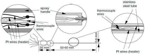
Figure 2. Sketch of the thermal conductivity probe.

Figure 3 shows the experimental setup, which is the same as the one used in Refs. [27,28,29,30].

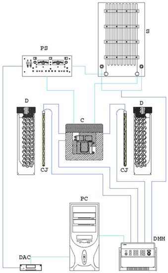
Figure 3. Experimental thermal conductivity setup.

The components of the experimental apparatus are (Figure 3):

• Shunt (S);
• Electrical generator (PS);
• Thermocouples;
• Data acquisition system: Keithley 2700 (DMM);
• Data converter: USB-6229 DAQ (DAC);
• Electronic calculator (PC);
• Platinum wire probe;
• Thermocouple on the wall of the measuring cell (to check the validity of the infinite medium hypothesis).

The temperature of the sample is kept constant by a thermostatically controlled fluid flowing around the measuring cell. The temperature of the fluid (a mixture of water and 67% ethylene glycol) is heated or cooled by a thermostatic bath.

During the measurement, the increase in the probe T is recorded as a function of time (t), and the slope a, which represents the linear portion of temperature versus time, is determined by linear regression. The sample k results from the following relation:

$$k=\frac{\dot{q}}{4\pi a}$$

(26)

Figure 4 shows a typical result of the temperature trend versus time.

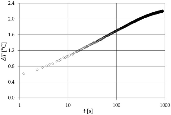
Figure 4. Typical temperature trend versus time of a thermal conductivity measurement.

The uncertainty analysis was evaluated according to the (ISO/IEC 1995), i.e., two types of uncertainty were evaluated, type A and B.

Type A uncertainty is derived from the test repetitions (five tests for each temperature for each sample) and from the standard deviation of the slope calculated by the least-square regression. The first type A uncertainty is much higher than the second, so only uncertainty due to the test repetitions was considered.

Type B uncertainty was also assessed and is mainly due to the prior knowledge of the experimenter. It was accurately assessed in Ref. [28] and resulted in an overall type B uncertainty of about 4 ÷ 5%.

Table 2 shows the thermal conductivity of the base fluid measured by the thermal probe method.

Table 2. Thermal conductivity of the base fluid.

T (°C)	kbf (W·m−1·K−1)
30	0.1530 ± 0.0006
40	0.1545 ± 0.0003
50	0.1567 ± 0.0002
60	0.1593 ± 0.0003

Three tests were carried out for each temperature, and Table 2 shows the average values. The measured thermal conductivity data agree with the reference values.

Table 3 shows the relative thermal conductivity of the nanofluids compared to the base fluid.

Table 3. Increase in thermal conductivity (SET-2).

φ (%)	T (°C)	k/kbf	φ (%)	T (°C)	k/kbf
0.04	30	1.0084	0.13	30	1.0275
	40	1.0168		40	1.0382
	50	1.0230		50	1.0428
	60	1.0251		60	1.0452
0.09	30	1.0183	0.17	30	1.0397
	40	1.0246		40	1.0505
	50	1.0306		50	1.0549
	60	1.0352		60	1.0596
0.22	30	1.0536
	40	1.0576
	50	1.0632
	60	1.0691

4. Discussion

4.1. SET-I

The data assumed for the models are listed in Table 4.

Table 4. Data from SET-I.

	φ (%)	a11/2 (nm)	p = a3/a1
Sample 3	1	40.5	1
Sample 4	3	52.5	1
Sample 5	1	5.0	8
Sample 6	3	5.0	8

• $k_p^{}=35\frac{\mathrm{W}}{\mathrm{m}\hspace{0.17em}\mathrm{K}}$, $k_{bf}^{}=0.161\frac{\mathrm{W}}{\mathrm{m}\hspace{0.17em}\mathrm{K}}$, T = 20 °C, $R_{bd}^{}={10}^{-8}\frac{{\mathrm{m}}^2\mathrm{K}}{\mathrm{W}}$ interfacial thermal resistance in agreement with Buongiorno et al. [12].
• $h=1\hspace{0.17em}\mathrm{n}\mathrm{m}\hspace{0.17em},\hspace{0.17em}{k}_l=2 k_{bf}$. In agreement with Liang et al. [31].
• $a_{11}$ minimum particle axis.
• $d_f=1.8\hspace{0.17em},\hspace{0.17em}{d}_l=1.4$. In agreement with Prasher et al. [24], d_l and d_f are chemical and fractal dimensions.

Remarks 1. 

➢

Geometric mean: this model was used in reverse (it allows the best estimate of m to be determined by the least-square regression).

➢

The Prasher model can be used for spherical nanoparticles. Samples 5 and 6 have needle-like particles, so the Prasher model was not used for these samples.

➢

The Prasher model was applied in direct and in reverse form. The inverse form is used, e.g., when the average number of particles per cluster N_int (or, alternatively, Rg/a) is the unknown parameter. In this case, the least-square regression allows the best N_int to be estimated. Direct use allows the thermal conductivity of the nanofluid to be determined once a value for N_int has been set.

➢

The Feng model predicts the thermal conductivity of the spherical nanoparticles, but Samples 5 and 6 have particles, which can be approximated by an ellipsoid. The generalized Feng model described in Section 2 was used.

Table 5 shows the increases in thermal conductivity (k/k_fb) predicted by the models. The following observations can be made:

Table 5. Increases in thermal conductivity k/k_fb predicted by the models.

Sample	H-C	Nan	Feng	Geometric Mean	Prasher
3	1.03	1.027	1.032	1.055 (m = 0)	1.041 (Nint = 2)
				1.039 (m = −0.14)	1.102 (Nint = 10)
4	1.091	1.083	1.1	1.1746 (m = 0)	1.127 (Nint = 2)
				1.121 (m = −0.14)	1.329 (Nint = 10)
5	1.047 *	1.07	1.055 **	1.053 (m = 0)	n.a.
				1.051 (m = −0.015)
6	1.144 *	1.211	1.163 *	1.169 (m = 0)	n.a.
				1.176 (m = −0.015)

* Computed with the general Feng model employing n as 3/Ψ = 4.7451; ** Assuming a value of d 10 nm; n.a. not applicable.

➢

The Nan model gives a maximum error of 3.5% (Sample 4);

➢

The Feng model makes fewer errors than the Nan model;

➢

The generalized Feng model agrees with the experimental data. Its error is 0.38% for Sample 5 and 1.12% for Sample 6;

➢

For the geometric mean, the values of “m” and a deviation from the zero value proposed by Turian [21] were collected. For the nanofluid couples (Samples 3–5 and 4–6), which have the same volumetric concentration, the shape of the nanoparticles is different. Homologous samples with spheroidal particles have a lower “m” than those with needle-like particles. The geometric mean model only explains the phenomenon related to volumetric concentration, temperature dependence on bulk thermal conductivity and particle size. Any other mechanism (microconvection, nanolayer, etc.) is considered within “m” if the choice of “m” accurately describes the experimental data.

➢

Using the Prasher model, the number of particles for a cluster equal to 2 was determined indirectly. However, this value does not seem to be accurate, as nanofluids of this type usually consist of a larger number of particles per cluster. In this case, the Feng model leads to a lower error than the Nan model. The Nan and Feng models qualitatively show an opposite trend in thermal conductivity as a function of particle size. This trend can be explained by the fact that the thermal conductivity in the Nan model depends inversely on the Kapitza thermal resistance, which increases with smaller particles. On the other hand, the thermal conductivity in Feng’s model depends directly on the presence of aggregates, which increase as the particles become smaller. Nan’s and Feng’s models differ significantly both when the dimensions of the nanoparticles are very small and when the volumetric concentration increases significantly (as will be seen in the next section).

➢

The formula for the geometric mean, Equation (10), used in an inverse mode, makes it possible to find the best estimate of m, which is closest to the experimental data. Such a procedure was not accurate in describing SET-1. Moreover, the procedure allows us to detect the effects of physical phenomena to be hidden in the variability of the parameter “m”. As a result, it is not possible to verify which phenomenon strongly influences the thermal conductivity of the nanofluid.

➢

If a higher number of particles per cluster were taken into account, the thermal conductivity predicted by the Prasher model would significantly overestimate the measured one. That this model overestimates the thermal conductivity may be due to the approximation of the backbone structure as ellipsoidal particles with the same aspect ratio.

➢

Nan’s and Feng’s models seem to be the simplest and give acceptable results. Problems arise when nanofluids have very small diameters of nanoparticles and very high volumetric concentrations. In the first case, the effect of particle size on thermal conductivity is uncertain. In the second case, the effect of volumetric concentration on thermal conductivity is well known. Although the tendency is the same for all models, the different models give different values for the thermal conductivity.

➢

Since the Feng model has a smaller error compared to the Nan model, it can be concluded that the scattering is negligible with respect to the phenomena of the cluster and of the nanolayer, which are considered in the Feng model. It was important to also extend the Feng model to the case of ellipsoidal particles (see Appendix A). For spherical particles, it showed the worst prediction among the models considered. The prediction of Feng for Sample 5 was k/k_bf = 1.034, and for Sample 6, k/k_fb = 1.101.

➢

Influence of microconvection: the tests were carried out at room temperature. With these values for temperature, particle diameter and concentration, microconvection is not significant.

➢

Influence of temperature: the data given were determined at room temperature. It is not possible to evaluate the influence on thermal conductivity.

4.2. SET-II

The parameters used in the models are the following:

• d = 50 nm.
• $R_{bd}={10}^{-8}\frac{{\mathrm{m}}^2\mathrm{K}}{\mathrm{W}}$ in agreement with Buongiorno et al. [12].
• h = 1 nm.
• $k_l=2 k_{bf}$ in agreement with Liang et al. [24].
• $d_f=1.8\hspace{0.17em},\hspace{0.17em}{d}_l=1.4$ in agreement with Prasher et al. [24].
• Electron density and Fermi velocity (relative to aluminum) equal to n_e = 18.1∙10²⁸ electrons/m³ and v_f = 2.03∙10⁶ m/s, respectively.
• The solidification temperature approximated to the scrolling point T_fr = −42 °C, in agreement with the technical data sheet of the base fluid Castrol Magnatec 10W40 A3/B4.

Table 6 reports the analytical prediction with the above assumptions.

Table 6. Thermal conductivity at different temperatures of the base fluid and particles.

T (°C)	kbf-exp (W·m−1·K−1)	kp * (W·m−1·K−1)
30	0.1530 ± 0.0006	33.4282
40	0.1545 ± 0.0003	33.4762
50	0.1567 ± 0.0002	33.5213
60	0.1593 ± 0.0003	33.5639

* Calculated with the Sommerfeld model and the Matthiessen rule [16].

Remarks 2. 

➢

Geometric mean: as the analysis of SET-1 shows, the parameter “m” does not change significantly. m = 0 was assumed, in agreement with Turian et al. [21].

➢

Prasher: the direct approach was chosen. A typical value for the number of particles per cluster was assumed, i.e., N_int = 10 particles/cluster.

➢

Corcione: since the solidification temperature of the base fluid was not available, the temperature of the scrolling point was assumed.

➢

The following values were used to calculate the Prandtl number of the base fluid in Equation (24) (Table 7).

Table 7. Thermophysical parameters assumed for the calculation of the Prandtl number in Equation (24).

T (°C)	cp (J·kg−1·K−1)	rbf (kg·m−3)	νbf·104 (m2·s−1)
30	2000	860	151.50
40	2034	850	101.00
50	2067	845	67.33
60	2100	840	52.00

Table 8 reports the analytical predictions, and Figure 5, Figure 6, Figure 7, Figure 8 and Figure 9 show the comparison between the theoretical predictions and the experimental data as a function of temperature and at different φ values.

Table 8. Comparison between experimental (SET-II) and theoretical results.

φ (%)	T (°C)	k/kbf (exp.)	k/kbf (theor.)
			Nan	Feng	Geom. Mean (m = 0)	Prasher (Nint = 10)	Corcione
0.04	30	1.0084 ± 0.0006	1.0009	1.0013	1.0022	1.0037	1.0085
	40	1.0168 ± 0.0003	1.0009	1.0013	1.0022	1.0037	1.0149
	50	1.0230 ± 0.0002	1.0009	1.0013	1.0021	1.0037	1.0217
	60	1.0251 ± 0.0003	1.0009	1.0013	1.0021	1.0037	1.0310
0.09	30	1.0183 ± 0.0006	1.0021	1.0029	1.0049	1.0083	1.0171
	40	1.0246 ± 0.0003	1.0021	1.0029	1.0049	1.0083	1.0254
	50	1.0306 ± 0.0002	1.0021	1.0029	1.0048	1.0083	1.0373
	60	1.0352 ± 0.0003	1.0021	1.0029	1.0048	1.0083	1.0530
0.13	30	1.0275 ± 0.0006	1.0031	1.0041	1.0070	1.0120	1.0218
	40	1.0382 ± 0.0003	1.0031	1.0041	1.0070	1.0120	1.0324
	50	1.0428 ± 0.0002	1.0031	1.0041	1.0070	1.0120	1.0476
	60	1.0452 ± 0.0003	1.0031	1.0041	1.0070	1.0120	1.0675
0.17	30	1.0397 ± 0.0006	1.0040	1.0054	1.0092	1.0158	1.0261
	40	1.0505 ± 0.0003	1.0040	1.0054	1.0092	1.0158	1.0387
	50	1.0549 ± 0.0002	1.0040	1.0054	1.0092	1.0158	1.0568
	60	1.0596 ± 0.0003	1.0040	1.0054	1.0091	1.0158	1.0806
0.22	30	1.0536 ± 0.0006	1.0052	1.0070	1.0119	1.0204	1.0309
	40	1.0576 ± 0.0003	1.0052	1.0070	1.0119	1.0204	1.0459
	50	1.0632 ± 0.0002	1.0052	1.0070	1.0119	1.0204	1.0673
	60	1.0691 ± 0.0003	1.0052	1.0070	1.0118	1.0204	1.0956

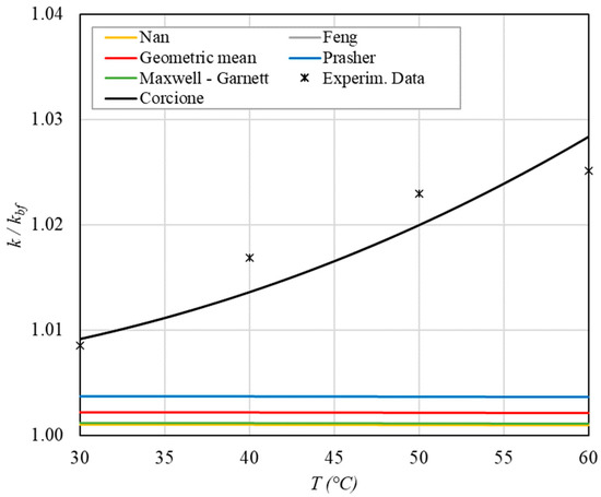
Figure 5. Increase in thermal conductivity as a function of temperature for φ = 0.04%.

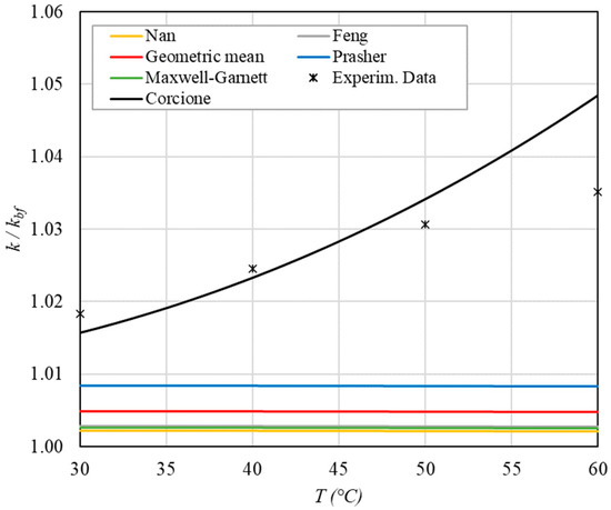
Figure 6. Increase in thermal conductivity versus temperature for φ = 0.09%.

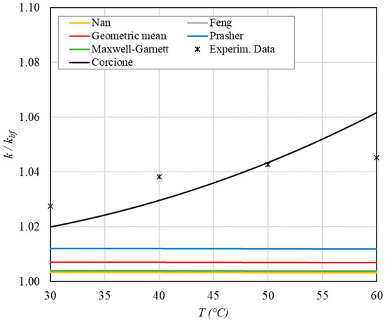
Figure 7. Increase in thermal conductivity versus temperature for φ = 0.13%.

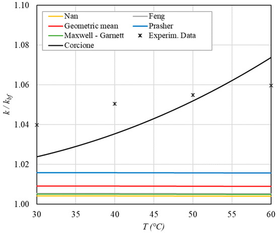
Figure 8. Increase in thermal conductivity versus temperature for φ = 0.17%.

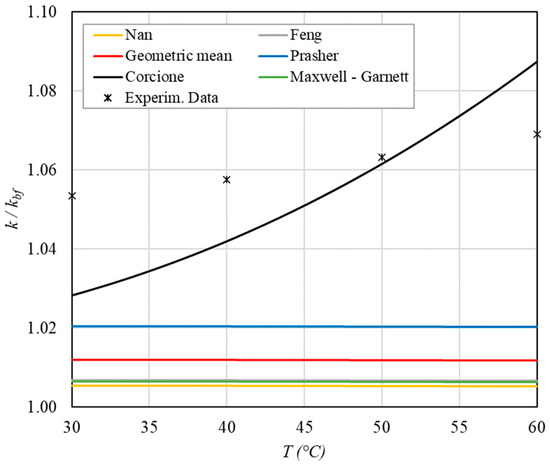
Figure 9. Increase in thermal conductivity versus temperature for φ = 0.22%.

The following observations can be made:

➢

The experimental enhancement in thermal conductivity ranges from a minimum of 0.8% to 6.9% as the volumetric concentration and temperature increase (Figure 5, Figure 6, Figure 7, Figure 8, Figure 9, Figure 10, Figure 11, Figure 12 and Figure 13). All the models considered, with the exception of Corcione, do not take into account the Brownian motion. These models have an error ranging from a minimum of 0.46% to 6.4%. The error is comparable to thermal conductive enhancement; consequently, these predictions lose their meaning.

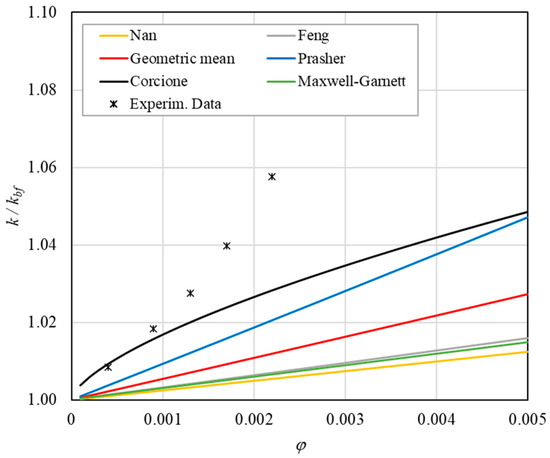Figure 10. Increase in thermal conductivity versus volumetric content for engine oil (Castrol Magnatec 10W40)—Alumina (d = 50 nm) at 30 °C.

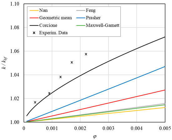Figure 11. Increase in thermal conductivity versus volumetric content for engine oil (Castrol Magnatec 10W40)—Alumina (d = 50 nm) at 40 °C.

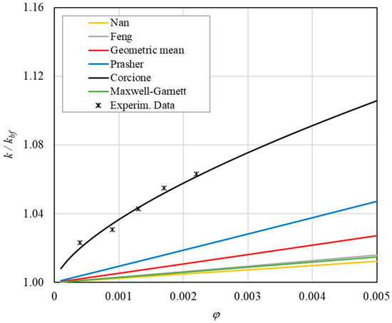Figure 12. Increase in thermal conductivity versus volumetric content for engine oil (Castrol Magnatec 10W40)—Alumina (d = 50 nm) at 50 °C.

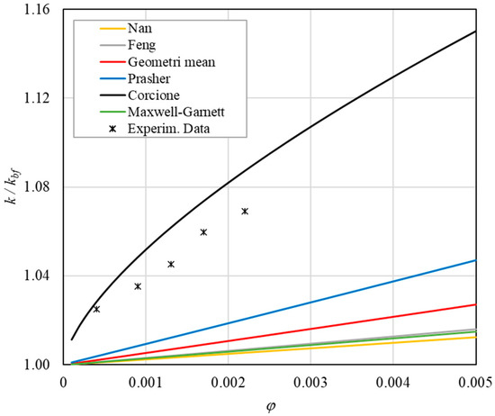Figure 13. Increase in thermal conductivity versus volumetric content for engine oil (Castrol Magnatec 10W40)—Alumina (d = 50 nm) at 60 °C.

➢

The Corcione model provides more accurate predictions. Its errors range from 0.13% to 2.2%.

➢

If the temperatures are sufficiently high (T > 30 °C), the Brownian motion must be taken into account to obtain more accurate predictions. It is therefore advisable to use theoretical models that take such phenomena into account, such as Corcione.

➢

When the volumetric concentration is very small (φ < 1%), the Nan, Feng, Prasher, the geometric mean (with n = 0) and H-C models underestimate the thermal conductivity acceptably at low temperatures, but at higher temperatures, the underestimation becomes non-negligible. The applicability of these models is limited to T ≤ 30 °C.

➢

Effect of volumetric content: it can be seen from Figure 10, Figure 11, Figure 12 and Figure 13 that the thermal conductivity at the same temperature increases by about 4–5% when the volumetric content is increased from 0.04 to 0.22%. However, from the experimental data, the growth rate is different at different temperatures. As the temperature is increased, the slope of the experimental data decreases from the case at T = 30 °C, where all the data are above the Corcione prediction, to the case at T = 60 °C, where all the data are below the Corcione prediction. In the middle case (T = 50 °C), the experimental data are almost perfectly described by the Corcione model. All the other models studied, i.e., Nan and Feng, show an average deviation of 3.61% and 3.51%, respectively, compared to the experimental results at the temperatures considered. This result shows that all the other theoretical models give results that are far from the experimental data. This result shows that there is a temperature range and a fraction value range where the microconvection effect is predominant compared to the other phenomena.

➢

The experimental results show a non-linear trend (Figure 10). Unlike the other models, which predict a linear trend in the concentration range of 0.04–0.22%, the effect of microconvection shows a non-linear increase at low volumetric concentrations, as highlighted by the Corcione model.

➢

Figure 5, Figure 6, Figure 7, Figure 8 and Figure 9 show the effect of temperature on thermal conductivity. An average increase of 1.4% was demonstrated with a temperature increase of 30 °C.

5. Conclusions

In this work, the main physical phenomena affecting the thermal conductivity of nanofluids were analyzed and highlighted. Two experimental data sets on the thermal conductivity of nanofluids—one taken from the literature and the other obtained experimentally—were used as reference for the analysis. The descriptions of the experimental data are supported by different theoretical models, each of which takes into account some physical phenomena and neglects others.

The following conclusions can be drawn:

➢

The comparison of SET-I with the models shows that clusters, the formation of the adsorbate nanolayer and the scattering of phonons at the solid–liquid interface are the most important phenomena to consider when φ = 1 ÷ 3. The Feng model is the most advisable model to use.

➢

The shape of the particles also matters because the Feng model must be generalized for particles with an ellipsoidal shape. The generalized model reported in this paper agrees with the experimental data and has an error of 0.38% for Sample 5 and 1.12% for Sample 6.

➢

The Feng model describes SET-I well, but not SET-II. This fact can be ascribed to the volume percentage of the nanoparticles and to the higher temperatures. SET-I has a volume percentage, which is an order of magnitude larger than SET-II. Consequently, microconvection at a very low percentage is significant for the phenomenon of clustering and the presence of the nanolayer. Indeed, the temperature is proportional to the Brownian motion. On the other hand, the volume percentage of the nanoparticle is proportional to the viscosity, and higher viscosity leads to a decrease in the Brownian motion.

➢

The comparison of SET-II with the models showed a significant influence of microconvection in the range of the volumetric concentrations studied. Corcione’s model approximates the measured values better than the other models. If microconvection can be neglected for volumetric concentrations above 0.005, the models of Nan and Feng are the most accurate, as they take into account more significant phenomena in this range of volumetric fraction. At a temperature of 50 °C and in the range of the volume fraction (0.04–0.22%), the experimental data are well reproduced by the Corcione model. For the other conditions, where microconvection cannot be neglected, the Corcione model gives the best prediction compared to the other models used but not the best fit with the experimental values. This is probably due to the empirical nature of this formulation. The physical conditions under which microconvection prevails were defined.

References

- Li, J.; Zhang, X.; Xu, B.; Yuan, M. Nanofluid research and applications: A review. Int. Commun. Heat Mass Transf. 2021, 127, 105543. [Google Scholar] [CrossRef]
- Sheremet, M.A. Applications of Nanofluids. Nanomaterials 2021, 11, 1716. [Google Scholar] [CrossRef] [PubMed]
- Sonawane, S.; Patankar, K.; Fogla, A.; Puranik, B.; Bhandarkar, U.; Kumar, S.S. An experimental investigation of thermophysical properties and heat transfer performance of Al2O3—Aviation Turbine Fuel nanofluids. Appl. Therm. Eng. 2011, 31, 2841–2849. [Google Scholar] [CrossRef]
- Li, Y.Y.; Lv, L.C.; Liu, Z.H. Influence of Nanofluids on the Operation Characteristics of Small Capillary Pumped Loop. Energy Convers. Manag. 2010, 51, 2312–2320. [Google Scholar] [CrossRef]
- Shukla, K.N. Heat Pipe for Aerospace Applications—An Overview. J. Electron. Cool. Therm. Control 2015, 5, 55065. [Google Scholar] [CrossRef]
- Choi, S.U.S. Enhancing thermal conductivity of fluids with nanoparticles. In Developments and Applications of Non-Newtonian Flows; Singer, D.A., Wang, H.P., Eds.; American Society of Mechanical Engineers: New York, NY, USA, 1995; Volume 231, pp. 99–105. [Google Scholar]
- Lee, S.; Choi SU, S.; Li, S.; Eastman, J.A. Measuring Thermal Conductivity of Fluids Containing Oxide Nanoparticles. J. Heat Transf. 1999, 121, 280–289. [Google Scholar] [CrossRef]
- Beck, M.; Yuan, Y.; Warrier, P.; Teja, A. The effect of particle size on the thermal conductivity of nanofluids. J. Nanoparticle Res. 2009, 11, 1129–1136. [Google Scholar] [CrossRef]
- Kokate, Y.D.; Sonawane, S.B. Investigation of particle size effect on thermal conductivity enhancement of distilled water—Al2O3 nanofluids. Fluid Mech. Res. Int. J. 2019, 3, 55–59. [Google Scholar] [CrossRef]
- Al-Hossainy, A.F.; Eid, M.R. Structure, DFT calculations and heat transfer enhancement in [ZnO/PG + H2O] C hybrid nanofluid flow as a potential solar cell coolant application in a double-tube. J. Mater. Sci. Mater. Electron. 2020, 31, 15243–15257. [Google Scholar] [CrossRef]
- Eid, M.R.; Al-Hossainy, A.F. Synthesis, DFT calculations, and heat transfer performance large-surface TiO2: Ethylene glycol nanofluid and coolant applications. Eur. Phys. J. Plus 2020, 135, 596. [Google Scholar] [CrossRef]
- Buongiorno, J.; Venerus, D.; Prabhat, N.; McKrell, T.; Townsend, J.; Christianson, R.; Tolmachev, Y.V.; Keblinski, P.; Hu, L.; Alvarado, J.L.; et al. A benchmark study on the thermal conductivity of nanofluids. J. Appl. Phys. 2009, 106, 094312. [Google Scholar] [CrossRef]
- Nan, C.W.; Birringer, R.; Clarke, D.; Gleiter, H. The Effective Thermal Conductivity or Particular Composites with Interfacial Thermal Resistance. J. Appl. Phys. 1997, 81, 6692. [Google Scholar] [CrossRef]
- Hamilton, R.L.; Crosser, O.K. Thermal Conductivity of Heterogeneous Two-Component Systems. Ind. Eng. Chem. Fundam. 1962, 1, 187–191. [Google Scholar] [CrossRef]
- Warrier, P.; Teja, A. Effect of particle size on the thermal conductivity of nanofluids containing metallic nanoparticles. Nanoscale Res. Lett. 2011, 6, 247. [Google Scholar] [CrossRef] [PubMed]
- Chopkar, M.; Sudarshan, S.; Das, P.; Manna, I. Effect of Particle Size on Thermal Conductivity of Nanofluid. Metall. Mater. Trans. A 2008, 39, 1535–1542. [Google Scholar] [CrossRef]
- Lenin, R.; Joy, P.; Bera, C. A review of the recent progress on thermal conductivity of nanofluid. J. Mol. Liq. 2021, 338, 116929. [Google Scholar] [CrossRef]
- Maxwell Garnett, J.C. Colours in Metal Glasses and in Metallic Films. Philos. Trans. R. Soc. A 1904, 203, 385–420. [Google Scholar] [CrossRef]
- Maxwell Garnett, J.C. Colours in Metal Glasses, in Metallic Films, and in Metallic Solutions. Philos. Trans. R. Soc. A 1905, 76, 237–288. [Google Scholar] [CrossRef]
- Kapitza, P.L. Heat Transfer and Superfluidity of Helium II. Phys. Rev. 1941, 60, 354. [Google Scholar] [CrossRef]
- Turian, R.M.; Sung, D.J.; Hsu, F.L. Thermal conductivity of granular coals, coal-water mixtures and multi-solid/liquid suspensions. Fuel 1991, 70, 1157–1172. [Google Scholar] [CrossRef]
- Sommerfeld, A. Zur elektronentheorie der metalle auf grund der fermischen statistic. Z. Für Phys. 1928, 47, 1–32. [Google Scholar] [CrossRef]
- Feng, Y.; Yu, B.; Zou, M. The effective thermal conductivity of nanofluids based on the nanolayer and the aggregation of nanoparticles. J. Phys. D Appl. Phys. 2007, 40, 3164. [Google Scholar] [CrossRef]
- Prasher, R.; Evans, W.; Meakin, P.; Fish, J.; Phelan, P.; Keblinski, P. Effect of aggregation on thermal conduction in colloidal nanofluids. Appl. Phys. Lett. 2006, 89, 143119. [Google Scholar] [CrossRef]
- Corcione, M. Empirical correlating equations for predicting the effective thermal conductivity and dynamic viscosity of nanofluids. Energy Convers. Manag. 2011, 52, 789–793. [Google Scholar] [CrossRef]
- Corasaniti, S.; Bovesecchi, G.; Gori, F. Experimental Thermal Conductivity of Alumina Nanoparticles in Water with and without Sonication. Int. J. Thermophys. 2021, 42, 23. [Google Scholar] [CrossRef]
- Bovesecchi, G.; Coppa, P. Basic Problems in Thermal-Conductivity Measurements of Soils. Int. J. Thermophys. 2013, 34, 1962–1974. [Google Scholar] [CrossRef]
- Coppa, P.; Pasquali, G. Thermal Conductivity of lipidic emulsions and its use for production and quality control. In Proceedings of the 2nd International Symposium on Instrumentation Science and Technology, Jinan, China, 20 August 2002; Volume 1, p. 486. [Google Scholar]
- Gori, F.; Corasaniti, S. Experimental Measurements and Theoretical Prediction of the Thermal Conductivity of Two- and Three-Phase Water/Olivine Systems. Int. J. Thermophys. 2003, 24, 1339–1353. [Google Scholar] [CrossRef]
- Bovesecchi, G.; Coppa, P.; Pistacchio, S. A new thermal conductivity probe for high temperature tests for the characterization of molten salts. Rev. Sci. Instrum. 2018, 89, 055107. [Google Scholar] [CrossRef]
- Liang, Z.; Tsai, H.L. Thermal conductivity of interfacial layers in nanofluids. Phys. Rev. E 2011, 83, 041602. [Google Scholar] [CrossRef]
- Wang, B.; Sheng, W.; Peng, X. A novel statistical clustering model for predicting thermal conductivity of nanofluid. Int. J. Thermophys. 2009, 30, 1992. [Google Scholar] [CrossRef]
Publisher’s Note: MDPI stays neutral with regard to jurisdictional claims in published maps and institutional affiliations. |
© 2022 by the authors. Licensee MDPI, Basel, Switzerland. This article is an open access article distributed under the terms and conditions of the Creative Commons Attribution (CC BY) license (https://creativecommons.org/licenses/by/4.0/).