Frequency Domain Design Method of the Aeroengine Fuel Servo Constant Pressure Difference Control System with High Performance

Abstract

The constant pressure difference regulating mechanism is widely used in aeroengine fuel servo metering systems, and it almost decides the metering precision. However, the design theory and design method of the available constant pressure difference regulating mechanism are unclear, and it is difficult to follow the high stability, high accuracy, and high robustness requirements of the modern aeroengine fuel servo metering system. In this paper, the design theory of the constant pressure difference regulating mechanism is revealed, and it indicates that it consists of two basic control units: a state feedback stabilization controller to ensure the asymptotic stability and disturbance rejection performance; and a servo and feed-forward compensator to ensure the asymptotic tracking ability. In addition, based on the frequency domain analysis method, the decisive influences about the control gains of the two control units on the dynamic performance and stability are analyzed. On this basis, a frequency domain design method of the two core control gains is proposed to complete the design task of the closed-loop system. The simulation results show that, under the adverse conditions of 1 MPa strong step disturbance of the inlet pressure and 50 mm² strong step disturbance of the variable inlet flow area, the steady-state working range of the controlled pressure difference meets 0.92 ± 0.01 MPa, the steady-state error is not more than 1%, the regulation time is not more than 0.01 s, the dynamic overshoot is not more than 10%, and the designed phase margin is more than 70°.

1. Introduction

The aeroengine control system is gradually transitioning from the hydraulic mechanical system to the digital electronic system. However, regardless of the hydraulic mechanical system or the digital electronic system, the fuel metering device primarily uses the constant pressure difference metering method, and the metering accuracy depends on the design performance of the constant pressure difference regulating mechanism. If the constant pressure difference regulating mechanism performs badly, it will cause aeroengine instability, such as speed and thrust swing, turbine overtemperature, and even compressor stall and surge [1]. With the proposal of the high stability, high accuracy, and high robustness performance requirements of the modern aeroengine control system, however, the traditional design methods cannot solve this high-tech problem because the design theory and design method of the available constant pressure difference regulating mechanism are unclear. Hence, the analysis and design research of the system has become a more core issue.

Research on the constant pressure difference regulating mechanism has mainly focused on modeling, simulation, and stability analysis. In the early stage, basis on the classical control theory, the dynamic equations and the transfer function block diagram were established. Meanwhile, the frequency domain model was obtained, and the static and dynamic characteristics were analyzed [2,3,4]. These works provide research basis, yet the frequency domain dynamic model is very complex, and they do not reveal the design theory as well as the relationship between the design parameters and the system performance. Additionally, there is a lack of test and simulation works. In recent years, with the development of simulation technology, research mainly focuses on dynamic modeling and simulation analysis, but the reports of theoretical research are still rare. For instance, the influences of the spring stiffness, hole diameter, and other parameters on the system performance are analyzed based on AMESim [5,6,7,8,9]. Unfortunately, these research works are carried out only on nonlinear models. Due to the lack of theoretical analysis to guide the research process, the main research method is the trial-and-error method, which is operated by changing the design parameters to explore the system performance, which is inefficient. Meanwhile, the influences of the oil return orifice profile structure on the system characteristics are deeply researched, and the study results show that the profile structure is related to the control gain of the system [10,11,12]. However, these researches do not involve system analysis and design but only provides guidance for the design of the orifice profile, which has limitations. Moreover, the stability conditions of the system are analyzed based on the transfer function models [13]. Problematically, the model is too simplified, and it lacks simulation or experimental verification, so the effectiveness of the method should be verified. Comfortingly, an optimal design of the variable orifice is studied by physical test, and the test results show that the variable orifice can bring better performance [14]. Although this study does not involve the design theory analysis, it is still instructive. In addition, based on the CFD simulation, the influences of the flow force on the balance of the motion valve are researched [15,16,17,18]. Indeed, the results show that the flow forces do have impacts on the dynamic performance of the system, but the impacts are not decisive. Additionally, there are some reports about the structure design of the pressure valves and the effect of the hysteresis on the speed fluctuation by physical test [19,20]. Nevertheless, this research lacks clear theoretical analysis and discussion of the results.

Although these researches are valuable, they are confined to classic analysis methods or to relying on simulation works, causing unclear design analysis results and inefficient guidance measures, and they are unable to realize the efficient design of the system. To solve the design problem, this paper firstly adopts the modern control theory to analyze the design theory of the system and proposes efficient guidance measures and design methods. The novelty of the work includes:

• Firstly, this paper adopts the linear incremental analysis method, which is based on the state space theory, and this method successfully reveals the design theory of the constant pressure difference regulating mechanism. The results clearly show that the system has three elements: the controlled object, the stabilization controller, and the servo and feed-forward compensator.
• Secondly, the precise state space models and frequency domain models of the system are established. On the basis concerning the advantage of frequency domain analysis methods, the accurate influences of the design parameters on the dynamic performance and stability of the system are analyzed, and the effective guidance measures are provided.
• Finally, a frequency domain design method of the core parameters is proposed, which includes the stabilization control gain and the servo control gain, and the method is proven to solve the design work efficiently and accurately.

The structure of this paper is as follows. In Section 2, the design theory and the compositions of the controller are provided, and the dynamic models are derived. In Section 3, the influences of the control gains on the dynamic performance and stability are clarified. In Section 4, the frequency domain design methods are provided. In Section 5, a design example is established. In Section 6, the conclusions are presented.

2. Design Theory and Dynamic Equations

Generally, the fuel flow metering formula of the fuel metering system is expressed as $Q=C_{q}A\sqrt{2\Delta P/\rho }$, and the metering principle is: ensure the pressure difference $\Delta P$ is a designed value, then determine the required fuel flow by controlling the flow area $A$ of the metering valve [13]. Independently, the flow area $A$ of the metering valve is controlled by a position control system, and, of course, the pressure difference $\Delta P$ is controlled by the constant pressure difference regulating mechanism. The structure of the constant pressure difference regulating mechanism is shown in Figure 1.

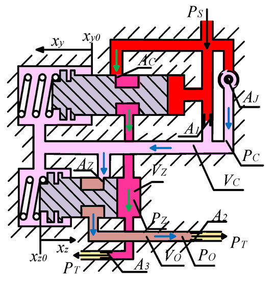
Figure 1. Structure diagram of the constant pressure difference regulating mechanism.

Where $P_S$ is the inlet pressure, $P_C$ is the controlled pressure, $P_Z$ is the regulating pressure, $P_O$ is the ejection pressure, $P_T$ is the return pressure, $A_J$ is the variable inlet flow area, $A_C$ is the variable compensated flow area, $A_Z$ is the variable regulating flow area, $A_1$ is the fixed inlet flow area, $A_2$ is the fixed ejection flow area, $A_3$ is the fixed outlet flow area, $V_C$ is the volume of the controlled chamber, $V_Z$ is the volume of the regulating chamber, $V_O$ is the volume of the ejection chamber, $x_y$ is the displacement of the compensated motion valve, and $x_z$ is the displacement of the regulating motion valve.

Illustratively, the controlled object is constructed by the fuel output path, which is represented by the blue arrows, and the fuel flow metering formula is expressed as $Q=C_q{A}_J\sqrt{2\left(P_S-P_C\right)/\rho }$. Generally, the regulation processes are that when the controlled pressure $P_C$ changes because of the disturbance of the inlet pressure $P_S$ or the flow area $A_J$, the compensated motion valve senses change of the pressure difference $\left(P_S-P_C\right)$ to regulate the compensated flow area $A_C$. Then, acting on the fuel regulating path, which is represented by the green arrows, the regulating pressure $P_Z$ changes, and the regulating motion valve senses change of the pressure difference $\left(P_Z-P_C\right)$ to regulate the regulating flow area $A_Z$, which is the control input of the controlled object, realizing the regulation of the controlled pressure $P_C$ [21,22,23,24,25,26].

2.1. Design Theory

The constant pressure difference regulating mechanism is a typical closed-loop servo tracking and disturbance rejection system. Its design objective is to ensure the controlled pressure increment $\Delta P_C$ servo tracks the inlet pressure increment $\Delta P_S$ and reject the disturbances caused by the variable inlet flow area increment $\Delta A_J$, and ensure that the controlled pressure increment difference $\left(\Delta P_S-\Delta P_C\right)$ is zero. Its design diagram is shown in Figure 2.

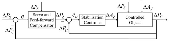
Figure 2. Design block diagram of the constant pressure difference regulating mechanism.

There are three basic regulation processes, as follows:

• Firstly, $\Delta P_S$ and $\Delta A_J$ are the disturbance inputs, and the disturbances caused by them are rejected through the regulation function of the stabilization controller.
• Secondly, $\Delta P_S$ is the reference input, and the controlled pressure increment $\Delta P_C$ servo tracks it through the regulation function of the servo compensator.
• Thirdly, $\Delta P_S$ is the feed-forward input, and the regulation ability of the system is improved, and the steady error is reduced.

2.2. Composition of the Controllers

The composition of the stabilization controller and the servo and feed-forward compensator is shown in Figure 3, and the derivation processes are shown in the following subsections.

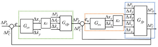
Figure 3. Composition of the controllers.

Where:

• $G_{fp}$ is the dynamic matrix of the controlled object.
• $G_{rv}$ is the dynamic matrix of the regulating motion valve, and $K_Z$ is the generalized stabilization control gain, and they construct the stabilization controller.
• $G_{cv}$ is the dynamic matrix of the compensated motion valve, $K_C$ is the generalized servo control gain, and $G_{cfp}$ is the dynamic matrix of the feed-forward compensated flow path, and they construct the servo and feed-forward compensator.

2.2.1. Controlled Object

The pressure-flow nonlinear dynamic equations of the controlled chamber and the ejection chamber are:

$$\frac{d{P}_C}{dt}=\frac{B}{V_C}·\left(\left(C_{qj}{A}_J+C_{q1}{A}_1\right)\sqrt{\frac{2(P_S-P_C)}{\rho }}-C_{qz}{A}_Z\sqrt{\frac{2(P_C-P_O)}{\rho }}+A_y{\dot{x}}_y-A_{zx}{\dot{x}}_z\right)$$

(1)

$$\frac{d{P}_O}{dt}=\frac{B}{V_O}·\left(C_{qz}{A}_Z\sqrt{\frac{2(P_C-P_O)}{\rho }}-C_{qo}{A}_2\sqrt{\frac{2(P_O-P_T)}{\rho }}\right)$$

(2)

where $B$ is the oil bulk modulus, $\rho$ is the oil density, and $C_q$ is the flow coefficient.

The calculation equation of the flow coefficient is:

$$C_q=C_{q\max }·\tanh (\sqrt{\frac{8\left|\Delta P\right|}{\rho }}·\frac{\rho ·d_h}{Nu·lamc})$$

(3)

where $C_{q\max }$ is the maximum flow coefficient, $d_h$ is the hydraulic diameter, $Nu$ is the absolute viscosity, and $lamc$ is the critical flow number.

The pressure-flow linear dynamic differential equations can be described as:

$$\Delta {\dot{P}}_C=\frac{B}{V_C}·\left(-(K_{PJ}+K_{PZ})·\Delta P_C+K_{PZ}·\Delta P_O+K_{AJ}·\Delta A_J+K_{PJ}·\Delta P_S-K_{AZ}·\Delta A_Z+A_y·\Delta {\dot{x}}_y-A_{zx}·\Delta {\dot{x}}_z\right)$$

(4)

$$\Delta {\dot{P}}_O=\frac{B}{V_O}·\left(-(K_{PZ}+K_{PT})·\Delta P_O+K_{PZ}·\Delta P_C+K_{AZ}·\Delta A_Z\right)$$

(5)

where $K_{AJ}=C_{qj}\sqrt{\frac{2(P_S-P_C)}{\rho }}$, $K_{AZ}=C_{qz}\sqrt{\frac{2(P_C-P_O)}{\rho }}$, $K_{PZ}=C_{qz}{A}_Z\sqrt{\frac{1}{2\rho (P_C-P_O)}}$, $K_{PT}=C_{qo}{A}_2\sqrt{\frac{1}{2\rho (P_O-P_T)}}$, $K_{PJ}=\left(C_{qj}{A}_J+C_{q1}{A}_1\right)\sqrt{\frac{1}{2\rho (P_S-P_C)}}$.

Then, the state space model of the controlled object is:

$$\begin{array}{l}\dot{x}=Ax+Bu+Ew\\ y=Cx+Du\end{array}$$

(6)

where $x={\left[\begin{array}{cc}\Delta P_C& \Delta P_O\end{array}\right]}^T$, $u={\left[\begin{array}{ccc}\Delta A_Z& \Delta {\dot{x}}_y& \Delta {\dot{x}}_z\end{array}\right]}^T$, $w={\left[\begin{array}{cc}\Delta A_J& \Delta P_S\end{array}\right]}^T$, $y=\left[\Delta P_C\right]$,

$$\begin{array}{l}A=\left[\begin{array}{cc}-\frac{B}{V_C}·(K_{PJ}+K_{PZ})& \frac{B}{V_C}·K_{PZ}\\ \frac{B}{V_O}·K_{PZ}& -\frac{B}{V_O}·(K_{PZ}+K_{PT})\end{array}\right]\\ B=\left[\begin{array}{ccc}-\frac{B}{V_C}·K_{AZ}& \frac{B}{V_C}·A_y& -\frac{B}{V_C}·A_{zx}\\ \frac{B}{V_O}·K_{AZ}& 0& 0\end{array}\right],E=\left[\begin{array}{cc}\frac{B}{V_C}·K_{AJ}& \frac{B}{V_C}·K_{PJ}\\ 0& 0\end{array}\right]\\ C=\left[\begin{array}{cc}1& 0\end{array}\right],D=\left[\begin{array}{ccc}0& 0& 0\end{array}\right]\end{array}$$

(7)

2.2.2. Stabilization Controller

A local coordinate for the regulating motion valve is established by taking the steady-state working point $x_{z0}=0$ as the local coordinate origin, $x_z$ as the relative displacement, and the arrow direction as the positive direction.

The motion nonlinear dynamic equation of the regulating motion valve is:

$$A_{zx}{P}_C-A_{zx}{P}_Z-M_z{\ddot{x}}_z-K_{f2}{\dot{x}}_z-K_2{x}_z-F_{L2}=0$$

(8)

where $M_z$ is the mass, $K_{f2}$ is the viscous friction coefficient, $K_2$ is the spring stiffness, $A_{zx}$ is the pressure bearing area, and $F_{L2}$ is the initial spring force.

The motion linear dynamic differential equation can be described as:

$$A_{zx}·\left(\Delta P_C-\Delta P_Z\right)-M_z·\Delta {\ddot{x}}_z-K_{f2}·\Delta {\dot{x}}_z-K_2·\Delta x_z=0$$

(9)

A function $A_Z=f_Z(x_{uz})$ is used to express the geometry design of the regulating motion valve orifice. According to its linearized gain characteristic $\Delta A_Z=\frac{d{f}_Z}{d{x}_{uz}}·\Delta x_{uz}$ and $\Delta x_{uz}=\Delta x_z$, the gain control law of the stabilization controller is indirectly expressed as:

$$\Delta A_Z=K_Z·\Delta x_z$$

(10)

where $K_Z=\frac{d{f}_Z}{d{x}_{uz}}$, and it is the generalized stabilization control gain.

Then, the state space model of the stabilization controller is:

$$\begin{array}{l}{\dot{x}}_{s1}=A_{s1}{x}_{s1}+B_{s1}y+E_{s1}{r}_{s1}\\ y_{s1}=C_{s1}{x}_{s1}+D_{s1}y+H_{s1}{r}_{s1}\end{array}$$

(11)

where $x_{s1}={\left[\begin{array}{cc}\Delta x_z& \Delta {\dot{x}}_z\end{array}\right]}^T$, $r_{s1}=\left[\Delta P_Z\right]$, $y_{s1}=\left[\Delta A_z\right]$,

$$\begin{array}{l}{A}_{s1}=\left[\begin{array}{cc}0& 1\\ -\frac{K_2}{M_z}& -\frac{K_{f2}}{M_z}\end{array}\right],B_{s1}=\left[\begin{array}{c}0\\ \frac{A_{zx}}{M_z}\end{array}\right],E_{s1}=\left[\begin{array}{c}0\\ -\frac{A_{zx}}{M_z}\end{array}\right]\\ C_{s1}=\left[\begin{array}{cc}{K}_Z& 0\end{array}\right],D_{s1}=\left[0\right],H_{s1}=\left[0\right]\end{array}$$

(12)

2.2.3. Servo and Feed-Forward Compensator

A local coordinate for the compensated motion valve is established by taking the steady-state working point $x_{y0}=0$ as the local coordinate origin, $x_y$ as the relative displacement, and the arrow direction as the positive direction.

The motion nonlinear dynamic equation of the compensated motion valve is:

$$A_y{P}_S-A_y{P}_C-M_y{\ddot{x}}_y-K_{f1}{\dot{x}}_y-K_1{x}_y-F_{L1}=0$$

(13)

where $M_y$ is the mass of the motion valve, $K_{f1}$ is the viscous friction coefficient, $K_1$ is the spring stiffness, $A_y$ is the pressure bearing area, and $F_{L1}$ is the initial spring force.

The motion linear dynamic differential equation can be described as:

$$A_y·\left(\Delta P_S-\Delta P_C\right)-M_y·\Delta {\ddot{x}}_y-K_{f1}·\Delta {\dot{x}}_y-K_1·\Delta x_y=0$$

(14)

A function $A_C=f_C(x_{uy})$ is used to express the geometry design of the compensated motion valve orifice. According to its linearized gain characteristics $\Delta A_C=\frac{d{f}_C}{d{x}_{uy}}·\Delta x_{uy}$ and $\Delta x_{uy}=\Delta x_y$, the gain control law of the servo compensator is indirectly expressed as:

$$\Delta A_C=K_C·\Delta x_y$$

(15)

where $K_C=\frac{d{f}_C}{d{x}_{uy}}$, and it is the generalized servo control gain.

The pressure-flow nonlinear dynamic equation of the regulating chamber is:

$$\frac{d{P}_Z}{dt}=\frac{B}{V_Z}·\left(C_{qc}{A}_C\sqrt{\frac{2(P_S-P_Z)}{\rho }}-C_{q3}{A}_3\sqrt{\frac{2(P_{\mathrm{Z}}-P_T)}{\rho }}+A_{ZX}{\dot{x}}_z\right)$$

(16)

The pressure-flow linear dynamic differential equation can be described as:

$$\Delta {\dot{P}}_Z=\frac{B}{V_Z}·\left(-(K_{PY}+K_{PT2})·\Delta P_Z+K_{AY}·\Delta A_C+K_{PY}·\Delta P_S+A_{ZX}·\Delta {\dot{x}}_z\right)$$

(17)

where $K_{AY}=C_{qc}\sqrt{\frac{2(P_S-P_Z)}{\rho }}$, $K_{PY}=C_{qc}{A}_C\sqrt{\frac{1}{2\rho (P_S-P_Z)}}$, $K_{PT2}=C_{q3}{A}_3\sqrt{\frac{1}{2\rho (P_Z-P_T)}}$.

Then, the state space model of the servo and feed-forward compensator is:

$$\begin{array}{l}{\dot{x}}_{s2}=A_{s2}{x}_{s2}+B_{s2}{u}_{s2}+E_{s2}r\\ y_{s2}=C_{s2}{x}_{s2}+D_{s2}{u}_{s2}+H_{s2}r\end{array}$$

(18)

where $x_{s2}={\left[\begin{array}{ccc}\Delta x_y& \Delta {\dot{x}}_y& \Delta P_Z\end{array}\right]}^T$, $u_{s2}={\left[\begin{array}{cc}\Delta P_C& \Delta {\dot{x}}_z\end{array}\right]}^T$, $r=\left[\Delta P_S\right]$, $y_{s2}=\left[\Delta P_Z\right]$,

$$\begin{array}{l}{A}_{s2}=\left[\begin{array}{ccc}0& 1& 0\\ -\frac{K_1}{M_y}& -\frac{K_{f1}}{M_y}& 0\\ \frac{B}{V_Z}·K_{AY}·K_C& 0& -\frac{B}{V_Z}·(K_{PY}+K_{PT2})\end{array}\right]\\ B_{s2}=\left[\begin{array}{cc}0& 0\\ -\frac{A_y}{M_y}& 0\\ 0& \frac{B}{V_Z}·A_{zx}\end{array}\right],E_{s2}=\left[\begin{array}{c}0\\ \frac{A_y}{M_y}\\ \frac{B}{V_Z}·K_{PY}\end{array}\right]\\ C_{s2}=\left[\begin{array}{ccc}0& 0& 1\end{array}\right],D_{s2}=\left[\begin{array}{cc}0& 0\end{array}\right],H_{s2}=\left[0\right]\end{array}$$

(19)

3. Frequency Domain Analysis

Concerning the advantage of the explicit description between the designed parameters and the performance when analyzed by transfer functions, the frequency domain analysis methods are used to analyze the quantitative influence of the designed parameters on the performance of the system [27,28]. The design block diagram of the closed-loop controlled loop is shown in Figure 4.

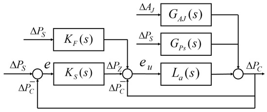
Figure 4. Loop design block diagram of the closed-loop system.

3.1. Design Analysis of the Stabilization Controller

The stabilization controller is used to ensure the asymptotic stability and disturbance rejection performance, and it acts on the inner loop. The analysis processes are as follows.

3.1.1. Calculation of the Open-Loop Transfer Function

The augmented open-loop state space model of the inner loop is:

$$\begin{array}{l}{\dot{x}}_a=A_a{x}_a+B_a{u}_a+E_{a}w\\ y=C_a{x}_a+D_a{u}_a\end{array}$$

(20)

where $x_a={\left[\begin{array}{cccc}\Delta x_z& \Delta {\dot{x}}_z& \Delta P_C& \Delta P_O\end{array}\right]}^T$, $u_a={\left[\begin{array}{cc}{e}_u& \Delta {\dot{x}}_y\end{array}\right]}^T$,

$$\begin{array}{l}{A}_a=\left[\begin{array}{cccc}0& 1& 0& 0\\ -\frac{K_2}{M_z}& -\frac{K_{f2}}{M_z}& 0& 0\\ -\frac{B}{V_C}·K_{AZ}·K_Z& -\frac{B}{V_C}·A_{zx}& -\frac{B}{V_C}·(K_{PJ}+K_{PZ})& \frac{B}{V_C}·K_{PZ}\\ \frac{B}{V_O}·K_{AZ}·K_Z& 0& \frac{B}{V_O}·K_{PZ}& -\frac{B}{V_O}·(K_{PZ}+K_{PT})\end{array}\right]\\ B_a=\left[\begin{array}{cc}0& 0\\ -\frac{A_{zx}}{M_z}& 0\\ 0& \frac{B}{V_C}·A_y\\ 0& 0\end{array}\right],E_a=\left[\begin{array}{cc}0& 0\\ 0& 0\\ \frac{B}{V_C}·K_{AJ}& \frac{B}{V_C}·K_{PJ}\\ 0& 0\end{array}\right]\\ C_a=\left[\begin{array}{cccc}0& 0& 1& 0\end{array}\right],D_a=\left[\begin{array}{cc}0& 0\end{array}\right]\end{array}$$

(21)

Defining

$$B_{a1}={\left[\begin{array}{cccc}0& -\frac{A_{zx}}{M_z}& 0& 0\end{array}\right]}^T$$

(22)

The open-loop transfer function of the inner loop is:

$$\begin{array}{l}{L}_a(s)=C_a{(sI-A_a)}^{-1}{B}_{a1}\\ =\frac{K_Z·\frac{A_{zx}}{M_z}·\frac{B}{V_C}·K_{AZ}·\left(s+\frac{B}{V_O}·K_{PT}\right)}{\left(\left(s+\frac{B}{V_C}·\left(K_{PJ}+K_{PZ}\right)\right)·\left(s+\frac{B}{V_O}·\left(K_{PZ}+K_{PT}\right)\right)-\frac{B}{V_C}·K_{PZ}·\frac{B}{V_O}·K_{PZ}\right)·\left(s^2+\frac{K_{f2}}{M_z}s+\frac{K_2}{M_z}\right)}\end{array}$$

(23)

3.1.2. Calculation of the Corner Frequencies

The performance of the system is determined by the corner frequencies of the frequency domain curve, and analyzing the accurate influences of the design parameters on the corner frequencies is the core idea. According to Equation (23), the corner frequencies of the frequency domain curve are calculated as follows.

• If $K_2>\frac{K_{f2}^2}{4·M_z}$, the second-order section is an underdamped oscillation link, and its poles are:

  $$p_{1,2}=-\frac{K_{f2}}{2·M_z}\pm j·\sqrt{\frac{K_2}{M_z}-{\left(\frac{K_{f2}}{2·M_z}\right)}^2}$$

  (24)
  The corner frequencies are defined as:

  $${\omega }_{1,2}=\frac{K_{f2}}{2·M_z}$$

  (25)
• If $K_2<\frac{K_{f2}^2}{4·M_z}$, the second-order section is an overdamped nonoscillation link, and its poles are:

  $$p_{1,2}=-\frac{K_{f2}}{2·M_z}\pm \sqrt{{\left(\frac{K_{f2}}{2·M_z}\right)}^2-\frac{K_2}{M_z}}$$

  (26)
  The corner frequencies are defined as:

  $${\omega }_{1,2}=\frac{K_{f2}}{2·M_z}\pm \sqrt{{\left(\frac{K_{f2}}{2·M_z}\right)}^2-\frac{K_2}{M_z}}$$

  (27)
  The third and fourth poles are:

  $$\begin{array}{l}{p}_{3,4}=-\frac{\left(\frac{B}{V_C}·\left(K_{PJ}+K_{PZ}\right)+\frac{B}{V_O}·\left(K_{PZ}+K_{PT}\right)\right)}{2}\\ \pm \sqrt{\left({\left(\frac{\left(\frac{B}{V_C}·\left(K_{PJ}+K_{PZ}\right)+\frac{B}{V_O}·\left(K_{PZ}+K_{PT}\right)\right)}{2}\right)}^2-\frac{B}{V_C}·\frac{B}{V_O}·\left(K_{PJ}·K_{PZ}+K_{PJ}·K_{PT}+K_{PZ}·K_{PT}\right)\right)}\end{array}$$

  (28)
  The corner frequencies are defined as:

  $$\begin{array}{l}{\omega }_{3,4}=\frac{\left(\frac{B}{V_C}·\left(K_{PJ}+K_{PZ}\right)+\frac{B}{V_O}·\left(K_{PZ}+K_{PT}\right)\right)}{2}\\ \pm \sqrt{\left({\left(\frac{\left(\frac{B}{V_C}·\left(K_{PJ}+K_{PZ}\right)+\frac{B}{V_O}·\left(K_{PZ}+K_{PT}\right)\right)}{2}\right)}^2-\frac{B}{V_C}·\frac{B}{V_O}·\left(K_{PJ}·K_{PZ}+K_{PJ}·K_{PT}+K_{PZ}·K_{PT}\right)\right)}\end{array}$$

  (29)
  The zero is:

  $$z_1=-\frac{B}{V_O}·K_{PT}$$

  (30)
  The corner frequency is defined as:

  $${\omega }_5=\frac{B}{V_O}·K_{PT}$$

  (31)
  The open-loop gain of the inner loop is:

  $$K_a=\frac{K_Z·\frac{A_{zx}}{M_z}·K_{AZ}·K_{PT}}{\left[\left(K_{PJ}+K_{PZ}\right)·\left(K_{PZ}+K_{PT}\right)-K_{PZ}·K_{PZ}\right]·\left(\frac{K_2}{M_z}\right)}$$

  (32)

The equations of the corner frequencies indicate that:

• The stabilization control gain $K_Z$ only affects the open-loop gain;
• The spring stiffness $K_2$ affects ${\omega }_1$, ${\omega }_2$, and the open-loop gain,
• The volume $V_C$ of the controlled chamber and the volume $V_O$ of the ejection chamber affect ${\omega }_3$, ${\omega }_4$, and ${\omega }_5$.

Designing the five corner frequencies and the open-loop gain is the key work. For example, to enhance the response performance and the disturbance rejection performance, the open-loop gain $K_a$ should be increased to make the magnitude curve move up, including:

• Increasing the stabilization control gain $K_Z$;
• Reducing the spring stiffness $K_2$;
• Increasing the pressure-bearing area $A_{zx}$.

3.1.3. Influence of the Stabilization Control Gain on the Frequency Domain Performance

Assuming $K_2<\frac{K_{f2}^2}{4·M_z}$ and only changing $K_Z$, by calculating the magnitude of the parameters ${\omega }_1$, ${\omega }_2$, ${\omega }_3$, ${\omega }_4$, ${\omega }_5$, and $K_Z$, the bode diagram curves are shown in Figure 5.

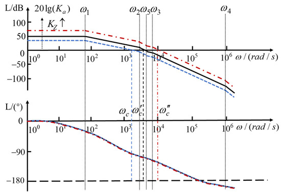
Figure 5. Bode diagram curves under different stabilization control gains.

When the stabilization control gain $K_Z$ increases, the magnitude curve moves up, and the phase curve remains unchanged, then:

• The steady-state gain $K_a$ increases according to Equation (32), and the steady error caused by disturbances is reduced, bringing a better disturbance rejection performance;
• The crossover frequency ${\omega }_c$ increases, and the settling time is reduced, bringing a faster response performance;
• The slope of the magnitude curve at the crossover frequency increases, and the damping ratio decreases, bringing a bigger overshoot;
• The phase margin decreases, bringing a worse robustness performance.

3.1.4. Stability Analysis

The characteristic polynomial of the inner closed-loop system is:

$$\begin{array}{ll}d(s)& =\left(\left(s+\frac{B}{V_C}·\left(K_{PJ}+K_{PZ}\right)\right)·\left(s+\frac{B}{V_O}·\left(K_{PZ}+K_{PT}\right)\right)-\frac{B}{V_C}·K_{PZ}·\frac{B}{V_O}·K_{PZ}\right)·\left(s^2+\frac{K_{f2}}{M_z}s+\frac{K_2}{M_z}\right)\\ & +\frac{d{f}_Z}{d{x}_{uz}}·\frac{A_{zx}}{M_z}·\frac{B}{V_C}·K_{AZ}·\left(s+\frac{B}{V_O}·K_{PT}\right)\end{array}$$

(33)

The equation is converted to:

$$d(s)=a_0{s}^4+a_1{s}^3+a_2{s}^2+a_3{s}^1+a_4$$

(34)

According to the stability conditions of the fourth-order system: all the coefficients of the characteristic polynomial should be positive, expressed as $a_i>0, i=0,1,2,3,4$, and

$$a_1{a}_2-a_0{a}_3>0$$

(35)

$$a_3\left(a_1{a}_2-a_0{a}_3\right)-a_4{a}_1^2>0$$

(36)

There is a stabilization control gain extremum that makes the inner loop system asymptotically stable, expressed as $K_{Z\max }$. Then, the stability condition of the inner loop is:

$$K_Z<K_{Z\max }$$

(37)

3.2. Design Analysis of the Servo and Feed-Forward Compensator

The servo and feed-forward compensator is used to ensure the asymptotic tracking ability, and it acts on the series loop. The analysis processes are as follows.

3.2.1. Calculation of the Open-Loop Transfer Function

Defining

$$B_{s3}={\left[\begin{array}{ccc}0& \frac{A_y}{M_y}& 0\end{array}\right]}^T$$

(38)

Then, the open-loop transfer function of the servo compensator from $e$ to $\Delta P_Z$ is:

$$K_S(s)=C_{s2}{(sI-A_{s2})}^{-1}{B}_{s3}=\frac{K_C·\frac{A_y}{M_y}·\frac{B}{V_Z}·K_{AY}}{\left(s+\frac{B}{V_Z}·(K_{PY}+K_{PT2})\right)·\left(s^2+\frac{K_{f1}}{M_y}s+\frac{K_1}{M_y}\right)}$$

(39)

3.2.2. Calculation of the Corner Frequencies

According to Equation (39), the corner frequencies of the frequency domain curve are calculated as follows.

• If $K>\frac{K_{f1}^2}{4·M_y}$, the second-order section is an underdamped oscillation link, and its poles are:

  $$p_{1,2}=-\frac{K_{f1}}{2·M_y}\pm j·\sqrt{\frac{K_1}{M_y}-{\left(\frac{K_{f1}}{2·M_y}\right)}^2}$$

  (40)
  The corner frequencies are defined as:

  $${\omega }_{1,2}=\frac{K_{f1}}{2·M_y}$$

  (41)
• If $K<\frac{K_{f1}^2}{4·M_y}$, the second-order section is an overdamped nonoscillation link, and its poles are:

  $$p_{1,2}=-\frac{K_{f1}}{2·M_y}\pm \sqrt{{\left(\frac{K_{f1}}{2·M_y}\right)}^2-\frac{K_1}{M_y}}$$

  (42)
  The corner frequencies are defined as:

  $${\omega }_{1,2}=\frac{K_{f1}}{2·M_y}\pm \sqrt{{\left(\frac{K_{f1}}{2·M_y}\right)}^2-\frac{K_1}{M_y}}$$

  (43)
  The third pole is:

  $$p_3=-\frac{B}{V_Z}·(K_{PY}+K_{PT2})$$

  (44)
  The corner frequency is defined as:

  $${\omega }_3=\frac{B}{V_Z}·(K_{PY}+K_{PT2})$$

  (45)
  The open-loop gain of the servo compensator is:

  $$K_e=\frac{K_C·\frac{A_y}{M_y}·K_{AY}}{\left(K_{PY}+K_{PT2}\right)·\frac{K}{M_y}}$$

  (46)

The equations of the corner frequencies indicate that:

• The control gain $K_C$ only affects the open-loop gain;
• The spring stiffness $K$ affects ${\omega }_1$, ${\omega }_2$, and the open-loop gain;
• The volume $V_Z$ of the regulating chamber affects ${\omega }_3$.

Designing the three corner frequencies and the open-loop gain is the key work. For example, to enhance the servo tracking performance of the system, the open-loop gain $K_e$ should be increased to make the magnitude curve move up, or the steady state gain of the feed-forward compensator should be increased, including:

• Increasing the control gain $K_C$;
• Reducing the spring stiffness $K_1$;
• Increasing the pressure-bearing area $A_y$;
• Increasing the compensated flow area $A_C$.

To enhance the stability margin of the system, the corner frequency ${\omega }_1$ and ${\omega }_2$ should be increased to make the phase curve move right, or the open-loop gain $K_e$ should be decreased to make the magnitude curve move down. In addition to adopting the measures contrary to the above measures, also included:

• Reducing the mass $M_y$ of the compensated motion valve;
• Increasing the viscous friction coefficient $K_{f1}$ of the compensated motion valve.

3.2.3. Influence of the Servo Control Gain on the Frequency Domain Performance

Assuming $K<\frac{K_{f1}^2}{4·M_y}$ and only changing $K_C$, the bode diagram curves are shown in Figure 6.

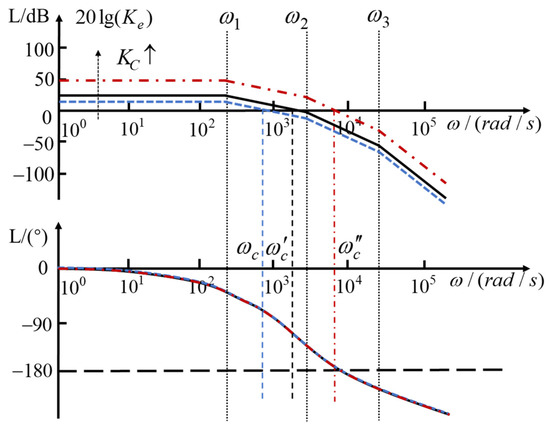
Figure 6. Bode diagram curves under different servo control gains.

When the control gain $K_C$ increases, the magnitude curve moves up, and the phase curve remains unchanged, then:

• The open loop gain $K_e$ increases according to Equation (46), and the steady error caused by reference input is reduced, bringing a better servo tracking performance;
• The crossover frequency ${\omega }_c$ increases, and the settling time is reduced, bringing a faster response performance;
• The slope of the magnitude curve at the crossover frequency increases, and the damping ratio decreases, bringing a bigger overshoot;
• The phase margin decreases, bringing a worse robustness performance.

3.3. Calculation of the Transfer Functions

It is inconvenient to calculate the output and error transfer functions by directly serializing the transfer functions obtained above, because there are coupling problems, and the simpler calculation method of the transfer functions are as follows.

The frequency domain loop design block diagram of the system is shown in Figure 7.

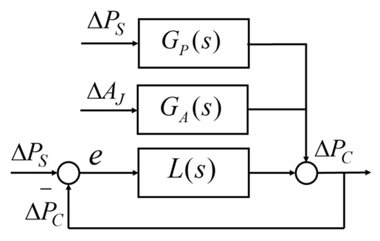
Figure 7. Frequency domain loop design block diagram of the system.

The open-loop state space model of the system is:

$$\begin{array}{l}{\dot{x}}_p=A_p·x_p+B_p·u_p+E_p·w\\ y=C_p·x_p+D_p·u_p+H_p·w\end{array}$$

(47)

where $x_p={\left[\begin{array}{ccccccc}\Delta x_y& \Delta {\dot{x}}_y& \Delta P_Z& \Delta x_z& \Delta {\dot{x}}_z& \Delta P_C& \Delta P_O\end{array}\right]}^T$, $u_p=[e]$, and

$$\begin{array}{l}{A}_p=\left[\begin{array}{ccccccc}0& 1& 0& 0& 0& 0& 0\\ -\frac{K_1}{M_y}& -\frac{K_{f1}}{M_y}& 0& 0& 0& 0& 0\\ \frac{B}{V_Z}·K_{AY}·K_C& 0& -\frac{B}{V_Z}·(K_{PY}+K_{PT2})& 0& \frac{B}{V_Z}·A_{zx}& 0& 0\\ 0& 0& 0& 0& 1& 0& 0\\ 0& 0& -\frac{A_{zx}}{M_z}& -\frac{K_2}{M_z}& -\frac{K_{f2}}{M_z}& \frac{A_{zx}}{M_z}& 0\\ 0& \frac{B}{V_C}·A_y& 0& -\frac{B}{V_C}·K_{AZ}·K_Z& -\frac{B}{V_C}·A_{zx}& -\frac{B}{V_C}·(K_{PJ}+K_{PZ})& \frac{B}{V_C}·K_{PZ}\\ 0& 0& 0& \frac{B}{V_O}·K_{AZ}·K_Z& 0& \frac{B}{V_O}·K_{PZ}& -\frac{B}{V_O}·(K_{PZ}+K_{PT})\end{array}\right]\\ B_p={\left[\begin{array}{ccccccc}0& \frac{A_y}{M_y}& 0& 0& 0& 0& 0\end{array}\right]}^T,E_p={\left[\begin{array}{ccccccc}0& 0& 0& 0& 0& \frac{B}{V_C}·K_{AJ}& 0\\ 0& 0& \frac{B}{V_Z}·K_{PY}& 0& 0& \frac{B}{V_C}·K_{PJ}& 0\end{array}\right]}^T\\ C_p=\left[\begin{array}{ccccccc}0& 0& 0& 0& 0& 1& 0\end{array}\right],D_p=\left[0\right],H_p=\left[\begin{array}{cc}0& 0\end{array}\right]\end{array}$$

(48)

The open-loop transfer function of the system is:

$$L(s)=C_p{(sI-A_p)}^{-1}{B}_p$$

(49)

Defining

$$\begin{array}{l}{E}_{p1}={\left[\begin{array}{ccccccc}0& 0& 0& 0& 0& \frac{B}{V_C}·K_{AJ}& 0\end{array}\right]}^T\\ E_{p2}={\left[\begin{array}{ccccccc}0& 0& \frac{B}{V_Z}·K_{PY}& 0& 0& \frac{B}{V_C}·K_{PJ}& 0\end{array}\right]}^T\end{array}$$

(50)

• The open-loop transfer function from $\Delta A_J$ to $\Delta P_C$ is $G_A(s)=C_p{(sI-A_p)}^{-1}{E}_{p1}$.
• The open-loop transfer function from $\Delta P_S$ to $\Delta P_C$ is $G_P(s)=C_p{(sI-A_p)}^{-1}{E}_{p2}$.

The sensitivity function and complementary sensitivity function of the system are defined as:

$$S={(I+L)}^{-1},T={(I+L)}^{-1}·L$$

(51)

Then, the control output transfer function of the system is:

$$\Delta P_C=(T+S·G_P)·\Delta P_S+S·G_A·\Delta A_J$$

(52)

When the control error is expressed as $e=\Delta P_S-\Delta P_C$, then it has:

$$e=(S-S·G_P)·\Delta P_S-S·G_A·\Delta A_J$$

(53)

4. Frequency Domain Design Method

Within the working range of the inlet pressure $P_S$ and the variable inlet flow area $A_J$, the design specifications of the steady-state and dynamic performance are:

• Steady-state performance: the designed pressure difference is $P_e$, and the phase margin is more than N °.
• Dynamic performance: the regulating time is not more than $t_s$, and the overshoot is not more than $\sigma$.

4.1. Calculation of the Control Gains

The system can be regarded as a fixed system with multiple stable working points which are determined by the inlet pressure $P_S$ and the variable inlet flow area $A_J$, and each working point has a fixed control gain. Therefore, the design method of gain scheduling is appropriate. The core idea is to determine the steady-state parameters first, and then design the control gain. The design processes are as follows.

4.1.1. Calculation of the Stabilization Control Gain

The steady-state flow balance equation of the controlled object is described as:

$$\left(C_{qj}{A}_J+C_{q1}{A}_1\right)\sqrt{\frac{2\left(P_S-P_C\right)}{\rho }}=C_{qz}{A}_Z\sqrt{\frac{2\left(P_C-P_O\right)}{\rho }}=C_{qo}{A}_2\sqrt{\frac{2\left(P_O-P_T\right)}{\rho }}$$

(54)

Assume the inlet pressure at a working point is $P_{S,i}$ and the inlet flow area is $A_{J,i}$. Since the design value of the pressure difference is $P_e$, there are:

$$P_{C,i}=P_{S,i}-P_e$$

(55)

$$P_{O,i}={\left(\frac{C_{qj,i}{A}_{J,i}+C_{q1,i}{A}_1}{C_{qo,i}{A}_2}\right)}^2·\left(P_{S,i}-P_{C,i}\right)+P_T$$

(56)

$$A_{Z,i}=\left(\frac{C_{qj,i}{A}_{J,i}+C_{q1,i}{A}_1}{C_{qz,i}}\right)\sqrt{\frac{\left(P_{S,i}-P_{C,i}\right)}{\left(P_{C,i}-P_{O,i}\right)}}$$

(57)

Then, the parameter values $K_{AJ,i}$, $K_{PJ,i}$, $K_{AZ,i}$, $K_{PZ,i}$, and $K_{PT,i}$ are obtained, and the open-loop transfer function of the inner loop system $L_{a,i}(s)$ is obtained.

According to Equation (37), there is a stabilization control gain extremum expressed as $K_{Z\max ,i}$, and it has:

$$K_{Z,i}<K_{Z\max ,i}$$

(58)

Subsequently, an appropriate stabilization control gain value $K_{Z,i}$ can be selected.

4.1.2. Calculation of the Servo Control Gain

The steady-state flow balance equation of the compensated flow path is described as:

$$C_{qc}{A}_C\sqrt{\frac{2(P_S-P_Z)}{\rho }}=C_{qt}{A}_3\sqrt{\frac{2(P_{\mathrm{Z}}-P_T)}{\rho }}$$

(59)

Then, according to the steady-state balance condition of the regulating motion valve:

$$0=A_{zx}{P}_{C,i}-A_{zx}{P}_{Z,i}-K_2{x}_{szd,i}$$

(60)

There are:

$$P_{Z,i}=P_{C,i}+\frac{K_2}{A_{zx}}·x_{szd,i}$$

(61)

$$A_{C,i}=\frac{C_{q3,i}{A}_3}{C_{qc,i}}\sqrt{\frac{(P_{Z,i}-P_T)}{(P_{S,i}-P_{Z,i})}}$$

(62)

Then, the parameter values $K_{AY,i}$, $K_{PY,i}$, and $K_{PT2,i}$ are obtained, and the transfer functions of the system $L_i(s)$, $e_i(s)$ are obtained. Additionally:

• There is a servo control gain extremum that makes the system asymptotically stable, expressed as $K_{C\max ,i}$, then it has:

  $$K_{C,i}<K_{C\max ,i}$$

  (63)
• There is a minimum control gain value that makes the system within the phase margin constraint, expressed as $K_{PH,i}$, then it has:

  $$K_{C,i}<K_{PH,i}$$

  (64)
• There is a control-gain working range that makes the system within the dynamic performance constraint expressed as $[K_{Cl,i},K_{Ch,i}]$, then it has:

  $$K_{Cl,i}<K_{C,i}<K_{Ch,i}$$

  (65)

Subsequently, an appropriate servo control gain value $K_{C,i}$ can be selected.

4.2. Geometry Design of the Orifices

4.2.1. The Regulating Motion Valve Orifice

The first spring compression of the regulating motion valve is designed as $x_{szd,1}$, and the designed relationship between the orifice underlap increment $\Delta x_{uz,i}$ and the area increment $(A_{Z,i}-A_{Z,i-1})$ is provided as:

$$\Delta x_{uz,i}=\frac{\left(A_{Z,i}-A_{Z,i-1}\right)}{K_{Z,i-1}}, i=2,3,\dots ,N$$

(66)

Then, the steady-state spring compression at the other working point is:

$$x_{szd,i}=x_{szd,i-1}+\Delta x_{uz,i}$$

(67)

where $N$ is number of the selected steady-state working points.

4.2.2. The Compensated Motion Valve Orifice

The above design processes are executed; then, the value pair $[A_{C,i},K_{C,i}]$ can be obtained. The designed relationship between the orifice underlap increment $\Delta x_{uy,i}$ and the area increment $(A_{C,i}-A_{C,i-1})$ is provided as:

$$\Delta x_{uy,i}=\frac{\left(A_{C,i}-A_{C,i-1}\right)}{K_{C,i-1}}, i=2,3,\dots ,N$$

(68)

4.3. Parameters Design of the Motion Valves

4.3.1. The Regulating Motion Valve

Assuming the initial spring compression is $x_{szd,0}$, if the initial orifice underlap of the regulating motion valve is $x_{uz,0}$, and the orifice underlap at the first working point is $x_{uz,1}$. Since $\Delta x_{uz}=\Delta x_{szd}$, then it has:

$$x_{szd,0}=x_{szd,1}-\left(x_{uz,1}-x_{uz,0}\right)$$

(69)

4.3.2. The Compensated Motion Valve

The steady-state balance condition of the compensated motion valve is expressed as:

$$0=A_y{P}_{S,i}-A_y{P}_{C,i}-K{x}_{scd,i}$$

(70)

Then, the steady-state spring compression at the first working point is:

$$x_{scd,1}=\frac{A_y}{K}{P}_e$$

(71)

Assuming the initial spring compression is $x_{scd,0}$, if the initial orifice underlap of the compensated motion valve is $x_{uy,0}$, and the orifice underlap at the first working point is $x_{uy,1}$. Since $\Delta x_{uy}=\Delta x_{scd}$, then it has:

$$x_{scd,0}=x_{scd,1}-\left(x_{uy,1}-x_{uy,0}\right)$$

(72)

5. Design Example

The known structural parameters of the constant pressure difference regulating mechanism are shown in Table 1.

Table 1. Structural parameters of the constant pressure difference regulating mechanism.

Parameter/Unit	Value	Parameter/Unit	Value
$M_y$/Kg	0.08	$M_z$/Kg	0.05
$K_1$/(N/m)	40,000	$K_2$/(N/m)	15,000
$K_{f1}$/(N/(m/s))	200	$K_{f2}$/(N/(m/s))	200
$d_y$/m	0.036	$d_z$/m	0.036
$A_1$/m2	2.827433 × 10−7	$V_C$/m3	2 × 10−6
$A_2$/m2	1.900664 × 10−4	$V_Z$/m3	2 × 10−6
$A_3$/m2	6.2831852 × 10−6	$V_O$/m3	4.908739 × 10−4
$\rho$/(Kg/m3)	780	$B$/bar	17,000
$Nu$/Pas	0.051	$lamc$	1000
$C_{q\max }$	0.7	$P_T$/bar	2

The working range of the inputs are:

• The working range of the inlet pressure $P_S$ is [3, 9] MPa;
• The working range of the variable inlet flow area $A_J$ is [10, 240] × 10⁻⁶ m².

The design objects are:

• The designed pressure difference $P_e$ is 0.92 ± 0.01 MPa, and the phase margin is more than 70°;
• The regulating time $t_s$ is not more than 0.01 s, and the overshoot is not more than 10%.

The design tasks are:

• Design the stabilization control law $A_Z=f_Z(x_{uz})$;
• Design the servo control law $A_C=f_C(x_{uy})$.

5.1. Dynamic Design of the First Working Point

5.1.1. Calculation of the Stabilization Control Gain

The inlet pressure at the first design point $P_{S,1}$ is 9 MPa, and the inlet flow area $A_{J,1}$ is 10 × 10⁻⁶ m². According to Equations (55)–(57), there are:

$$P_{C,1}=P_{S,1}-\Delta P_e=8.08 \mathrm{MPa}$$

(73)

$$P_{O,1}={\left(\frac{C_{qj,1}{A}_{J,1}+C_{q1,1}{A}_1}{C_{qo,1}{A}_2}\right)}^2·\left(P_{S,1}-P_{C,1}\right)+P_T=0.20265028 \mathrm{MPa}$$

(74)

$$A_{Z,1}=\left(\frac{C_{qj,1}{A}_{J,1}+C_{q1,1}{A}_1}{C_{qz,1}}\right)\sqrt{\frac{\left(P_{S,1}-P_{C,1}\right)}{\left(P_{C,1}-P_{O,1}\right)}}=3.4862689·{10}^{-6}{ \mathrm{m}}^2$$

(75)

Then, the values of the parameters $K_{AJ,1}$, $K_{PJ,1}$, $K_{AZ,1}$, $K_{PZ,1}$, and $K_{PT,1}$ are obtained. According to Equation (58), it has:

$$K_{Z,1}<K_{Z\max ,1}=0.07609$$

(76)

5.1.2. Calculation of the Servo Control Gain

The steady-state spring compression of the regulating motion valve at the first working point $x_{szd,1}$ is designed as 10 mm; then, according to Equation (61), it has:

$$P_{Z,1}=P_{C,1}+\frac{K_2}{A_{zx}}·x_{szd,1}=8.2273657 \mathrm{MPa}$$

(77)

Then, the parameter values $K_{AY,1}$, $K_{PY,1}$, and $K_{PT2,1}$ are obtained, and the transfer functions of the system are obtained.

When selecting different $K_{Z,1}$, according to Equations (63)–(65), the values of the parameters $K_{C\max ,1}$, $K_{PH,1}$, and $[K_{Cl,1},K_{Ch,1}]$ can be obtained, as shown in Table 2.

Table 2. The constraint values of the servo control gain at the first working point.

${\mathit{K}}_{\mathit{Z},1}$	${\mathit{K}}_{\mathit{C}\mathbf{max},1}$	$[{\mathit{K}}_{\mathit{C}\mathit{l},1},{\mathit{K}}_{\mathit{C}\mathit{h},1}]$	${\mathit{K}}_{\mathit{P}\mathit{H},1}$
0.0005	4.61	(0.06, 3.30)	0.49
0.001	4.60	(0.03, 3.20)	0.49
0.005	4.56	(0.02, 3.20)	0.50
0.010	4.50	(0.02, 3.20)	0.50
0.015	4.44	(0.02, 3.20)	0.50
0.020	4.38	(0.01, 3.20)	0.50

Finally, the stabilization control gain $K_{Z,1}$ is designed as 0.01, and the servo control gain $K_{C,1}$ is designed as 0.05.

5.2. Dynamic Design of Other Working Points

Here, $4\times 5$ steady-state working points are selected, as shown in Table 3.

Table 3. The extrema of the stabilization control gain at every working point.

${\mathit{P}}_{\mathit{S}}$ MPa	${\mathit{A}}_{\mathit{J}}$ mm2	${\mathit{A}}_{\mathit{Z}}$ mm2	${\mathit{K}}_{\mathit{Z}\mathbf{max}}$
3	10	7.1413178	0.276
	30	21.258905	2.560
	80	58.720918	26.510
	160	138.75330	239.530
	240	359.53286	5574.50
5	10	4.9691655	0.1328
	30	14.750547	1.188
	80	39.904931	10.328
	160	85.546194	59.495
	240	148.38949	235.570
7	10	4.0360839	0.0944
	30	11.969912	0.834
	80	32.175269	6.792
	160	67.213819	34.532
	240	109.70300	107.490
9	10	3.4862689	0.07609
	30	10.334703	0.668
	80	27.693258	5.255
	160	57.160884	25.153
	240	90.995231	71.128

• The stabilization control gain extrema that make the inner loop system stable are shown in Table 3.
• The design processes in Section 4.1 are executed; then, the value pair $[A_{Z,i},K_{Z,i}]$ can be obtained, as shown in Table 4.
  Table 4. The value pair of the stabilization controller at every working point.

  No.	${\mathit{A}}_{\mathit{Z}}$ mm2	${\mathit{K}}_{\mathit{Z}}$	$\mathbf{\Delta }{\mathit{x}}_{\mathit{u}\mathit{z}}$ mm	${\mathit{A}}_{\mathit{C}}$ mm2
  1	3.4862689	0.0100	0	20.252534
  2	4.0360839	0.0115	0.054981500	17.559553
  3	4.9691655	0.0130	0.136119030	14.367214
  4	7.1413178	0.0145	0.303207669	10.215733
  5	10.334703	0.0130	0.523441131	20.364172
  6	11.969912	0.0120	0.649226439	17.672847
  7	14.750547	0.0130	0.880946022	14.490336
  8	21.258905	0.0140	1.381588945	10.363465
  9	27.693258	0.0130	1.841185588	20.652604
  10	32.175269	0.0135	2.185955665	17.974697
  11	39.904931	0.0125	2.758523220	14.812128
  12	57.160884	0.0110	4.138999460	21.182637
  13	58.720918	0.0125	4.280820733	10.781931
  14	67.213819	0.0130	4.960252813	18.554773
  15	85.546194	0.0135	6.370435505	15.482255
  16	90.995231	0.0140	6.774067876	21.837585
  17	109.70300	0.0150	8.110337090	19.275786
  18	138.75330	0.0175	10.04702376	11.723734
  19	148.38949	0.0190	10.59766319	16.368022
  20	359.53286	0.0200	21.71047213	14.305249

• The design processes in Section 4.1 are executed; then, the value pair $[A_{C,i},K_{C,i}]$ can be obtained, as shown in Table 5.
  Table 5. The value pair of the servo controller at every working point.

  ${\mathit{P}}_{\mathit{S}}$ MPa	${\mathit{A}}_{\mathit{J}}$ mm2	${\mathit{A}}_{\mathit{C}}$ mm2	${\mathit{K}}_{\mathit{C}\mathbf{max}}$	$[{\mathit{K}}_{\mathit{C}\mathit{l}},{\mathit{K}}_{\mathit{C}\mathit{h}}]$	${\mathit{K}}_{\mathit{P}\mathit{H}}$	${\mathit{K}}_{\mathit{C}}$	Margin/°
  3	10	10.215733	3.79	(0.02, 1.50)	0.41	0.05	96.6
  	30	10.363465	3.55	(0.02, 0.75)	0.25	0.05	96.9
  	80	10.781931	3.74	(0.02, 0.55)	0.17	0.05	102.0
  	160	11.723734	3.56	(0.03, 0.45)	0.15	0.05	107.0
  	240	14.305249	2.74	(0.04, 0.50)	0.20	0.05	117
  5	10	14.367214	4.06	(0.02, 2.10)	0.46	0.05	101.0
  	30	14.490336	3.40	(0.02, 1.55)	0.27	0.05	98.3
  	80	14.812128	3.28	(0.02, 1.25)	0.18	0.05	102.0
  	160	15.482255	3.47	(0.03, 1.10)	0.15	0.05	106.0
  	240	16.368022	3.36	(0.03, 0.85)	0.13	0.05	93.7
  7	10	17.559553	4.29	(0.02, 3.10)	0.49	0.05	104.0
  	30	17.672847	3.34	(0.02, 2.55)	0.28	0.05	99.9
  	80	17.974697	2.97	(0.02, 2.10)	0.17	0.05	103.0
  	160	18.554773	3.12	(0.03, 2.05)	0.14	0.05	104.0
  	240	19.275786	3.24	(0.03, 1.75)	0.12	0.05	87.0
  9	10	20.252534	4.50	(0.02, 3.20)	0.50	0.05	106.0
  	30	20.364172	3.27	(0.02, 2.95)	0.29	0.05	102.0
  	80	20.652604	2.79	(0.02, 2.25)	0.17	0.05	104.0
  	160	21.182637	2.94	(0.03, 2.15)	0.14	0.05	105.0
  	240	21.837585	2.97	(0.03, 2.05)	0.10	0.05	79.6

5.3. Parameters Design of the Valves

5.3.1. Parameters Design of the Regulating Motion Valve

The designed initial orifice underlap of the regulating motion valve $x_{uz,0}$ is 0.1 mm, and the designed orifice underlap at the initial working point $x_{uz,1}$ is 0.1 mm. According to Equation (69), it has:

$$x_{szd,0}=x_{szd,1}-\left(x_{uz,1}-x_{uz,0}\right)=10 \mathrm{mm}$$

(78)

5.3.2. Parameters Design of the Compensated Motion Valve

According to Equation (71), the steady-state spring compression at the first working point is:

$$x_{scd,1}=\frac{A_y}{K}{P}_e=23.411148 \mathrm{mm}$$

(79)

The designed initial orifice underlap of the compensated motion valve $x_{uy,0}$ is 0.1 mm, and the designed orifice underlap at the initial working point $x_{uy,1}$ is 0.1 mm. According to Equation (72), it has:

$$x_{scd,0}=x_{scd,1}-\left(x_{uy,1}-x_{uy,0}\right)=23.411148 \mathrm{mm}$$

(80)

5.3.3. Geometry Design of the Orifices

According to Equations (66) and (68), the geometry design of the orifices are shown in Table 6.

Table 6. Geometry design of the compensated orifice and the regulating orifice.

${\mathit{x}}_{\mathit{u}\mathit{z}}$ mm	${\mathit{A}}_{\mathit{Z}}$ mm2	${\mathit{x}}_{\mathit{u}\mathit{y}}$ mm	${\mathit{A}}_{\mathit{C}}$ mm2
0	0	0	0
0.1	3.4862689	0.20431466	10.215733
0.154981500	4.0360839	0.2072693	10.363465
0.236119030	4.9691655	0.21563862	10.781931
0.403207669	7.1413178	0.23447468	11.723734
0.623441131	10.334703	0.28610498	14.305249
0.749226439	11.969912	0.28734428	14.367214
0.980946022	14.750547	0.28980672	14.490336
1.481588945	21.258905	0.29624256	14.812128
1.941185588	27.693258	0.3096451	15.482255
2.285955665	32.175269	0.32736044	16.368022
2.858523220	39.904931	0.35119106	17.559553
4.238999460	57.160884	0.35345694	17.672847
4.380820733	58.720918	0.35949394	17.974697
5.060252813	67.213819	0.37109546	18.554773
6.470435505	85.546194	0.38551572	19.275786
6.874067876	90.995231	0.40505068	20.252534
8.210337090	109.70300	0.40728344	20.364172
10.14702376	138.75330	0.41305208	20.652604
10.69766319	148.38949	0.42365274	21.182637
21.81047213	359.53286	0.4367517	21.837585

Additionally, the geometry relationship of the flow area and the underlap of the two orifices are shown in Figure 8a and Figure 8b, respectively.

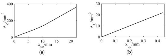
Figure 8. (a) Geometry design curve for the underlap and the flow area of the regulating orifice; (b) geometry design curve for the underlap and the flow area of the compensated orifice.

5.4. Simulation and Discussion

The simulation works are carried out on the nonlinear model as shown in Figure 9, which can be established based on AMESim, and the structural parameters and design parameters are set.

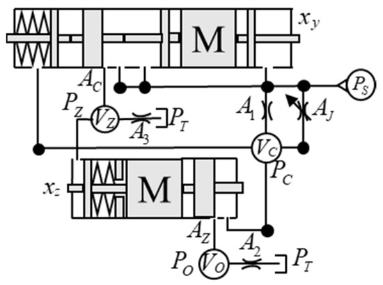
Figure 9. Nonlinear model of the constant pressure difference regulating mechanism.

5.4.1. Simulation

• Within the working range of the inputs, set the variable inlet flow area input $A_J$ as 10 mm², 50 mm², 100 mm², 150 mm², 200 mm², and 240 mm², respectively, and give the inlet pressure step input signal as shown in Figure 10. The simulation results are shown in Figure 11.
  

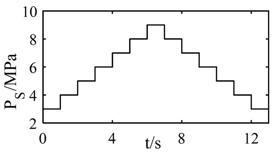  Figure 10. Input curve of the inlet pressure.
  

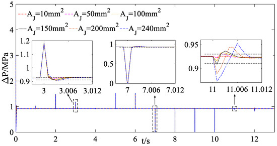  Figure 11. Step response curves of the inlet pressure disturbance.
• Within the working range of the inputs, set the inlet pressure input $P_S$ as 3 MPa, 4 MPa, 5 MPa, 6 MPa, 7 MPa, 8 MPa, and 9 MPa, respectively, and give the variable inlet flow area step input signal, as shown in Figure 12. The simulation results are shown in Figure 13.
  

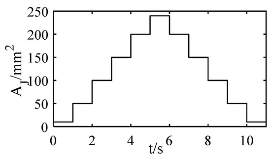  Figure 12. Disturbance input curve of the inlet flow area.
  

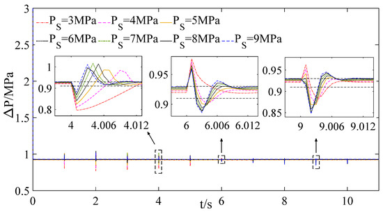  Figure 13. Step response curves of the inlet flow area disturbance.

The results show that, under different inlet pressure step disturbances and different inlet flow area step disturbances, the steady-state working range of the controlled pressure difference is 0.92 ± 0.01 MPa, the steady-state error is not more than 1%, the dynamic regulating time is not more than 0.01 s, and the overshoot is not more than 10%.

5.4.2. Discussion

Evidently, the steady and dynamic performance all meet the design requirements. Especially, the steady-state error is very small, and the dynamic characteristics of most design points are consistent with the theoretical design because of the precise models, which verify that the proposed methods are correct and accurate.

However, according to the preceding step response curves, it can be found that, for the design points close to the working boundary, such as the inlet pressure input $P_S$ as 3 MPa and the inlet flow area input $A_J$ as 240 mm², the dynamic characteristics are very different from those design points far away from the working boundary. Especially, the settling time increases and the overshoot increases.

This is a typical nonlinear phenomenon, and the reason can be explained from the following compensated flow area output curves, as shown in Figure 14 and Figure 15.

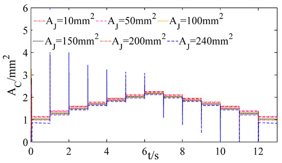
Figure 14. Compensated flow area output curves of the inlet pressure disturbance.

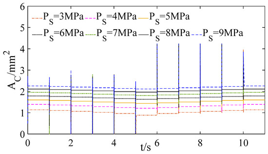
Figure 15. Compensated flow area output curves of the inlet flow area disturbance.

Combining Figure 11 with Figure 14, the compensated flow area at 3 s and 7 s is far from the boundary value 0, and the system does not enter the nonlinear state; hence, the step response characteristics are consistent with the theoretical design. However, the compensated flow area at 11 s reaches the nonlinear boundary, and the controller loses the regulating ability, causing the settling time and the overshoot to increase.

Similarly, combining Figure 13 with Figure 15, the nonlinear characteristic of the compensated flow area also impacts the step response of the inlet flow area disturbance. It follows that, in the design process of controllers, nonlinearity is also a very crucial factor, which needs to be paid enough attention to.

6. Conclusions

Based on the linear incremental analysis method, this paper reveals the design theory of the constant pressure difference regulating mechanism and proposes the frequency domain analysis and design methods of the system. The simulation results of the nonlinear model verify the accuracy of the proposed methods, and the conclusions are as follows:

• Compared with the classic analysis method based on direct transfer function transformation, the linear incremental method is based on the state space, and it is clearer to reveal the design theory of the constant pressure difference regulating mechanism. Furthermore, the analysis method also clarifies the key design parameters, including the stabilization control gain and the servo control gain, which was not involved in previous research.
• Concerning the advantage of the explicit description between the designed parameters and the performance when analyzed by the loop transfer functions, the frequency domain analysis method clearly describes the quantitative influence of the control gains on the frequency domain performance of the closed-loop system and provides more correct guidance for the design of the performance parameters, avoiding trial and error in simulation research.
• The simulation results show that the steady and dynamic performance all meet the design requirements when utilizing the proposed frequency domain design method; especially, the steady-state error is very small, and the phase margin is very large, which are beyond the design requirements. Evidently, the proposed design methods are correct and accurate and can be widely applied in the analysis and predesign of other components of the fuel metering system, such as the constant pressure control system and the position control system.

Nevertheless, the proposed methods may not work as perfect as the simulation tests when implementing actual physical tests, which should be verified in the future research. Furthermore, it is also interesting to research the controller design method when considering the nonlinear characteristics, which will be explored in future works.

References

- Yang, F.; Wang, X.; Cheng, T.; Liu, X. Dynamic characteristics analysis of a pressure differential valve. Aeroengine 2015, 41, 44–50. [Google Scholar] [CrossRef]
- Ma, C.Y. The analysis and design of hydraulic pressure-reducing valves. J. Eng. Ind. 1967, 89, 301. [Google Scholar] [CrossRef]
- Fan, R.; Zhang, M. The establishment of pilot-operated relief valve’s dynamic mathematic model and the dynamic properties analysis. J. Zheng Zhou Text. Inst. 1997, 3, 58–61. [Google Scholar]
- Wu, D.; Burton, R.; Schoenau, G.; Bitner, D. Analysis of a pressure—Compensated flow control valve. J. Dyn. Syst. Meas. Control. 2007, 129, 203–211. [Google Scholar] [CrossRef]
- Wen, Y.J. Analysis of characteristics of oil return differential pressure valve with EASY5. In Proceedings of the 11th Symposium on Automatic Engine Control of CAA, Beijing, China, 8–10 November 2002; pp. 21–26. [Google Scholar]
- Hong, W.; Liu, H.L.; Wang, G.Z.; Qin, J. Research on pressure characteristics of relief valve without pressure overshoot. Chin. Hydraul. Pneum. 2012, 10, 104–106. [Google Scholar] [CrossRef]
- Shang, Y.; Guo, Y.Q.; Wang, L. Study of impact of design parameter of differential pressure controller on fuel metering system. Aeronaut. Manuf. Technol. 2013, 6, 89–91. [Google Scholar] [CrossRef]
- Hang, J.; Li, Y.Y.; Yang, L.M.; Li, Y.H. Design and Simulation of Large Flowrate Fuel Metering Valve of Aero engine Based on AMESim. In Proceedings of the 2020 15th IEEE Conference on Industrial Electronics and Applications (ICIEA), Kristiansand, Norway, 9–13 November 2020; IEEE: Piscataway, NJ, USA, 2020. [Google Scholar] [CrossRef]
- Wang, B.; Zhao, H.C.; Ye, Z.F. AMESim simulation of afterburning metering unit for fuel system. Aeroengine 2014, 40, 62–66. [Google Scholar] [CrossRef]
- Zeng, D.T.; Wang, X.; Tan, D.L.; Xu, M. Fuel scavenger contour performance analysis of fuel metering devices. Aeroengine 2010, 36, 38. [Google Scholar] [CrossRef]
- Zeng, D.T.; Wang, X. Design and analysis of characteristics of damping hole for a fuel metering valve. In Proceedings of the 2010 International Conference on Mechanical and Electrical Technology, Kyoto, Japan, 1–3 August 2010; IEEE: Piscataway, NJ, USA, 2010. [Google Scholar] [CrossRef]
- Zeng, D.T.; Wang, X.; Tan, D.L. Effects of fuel returned shape on metering devices characteristics. Aeroengine 2012, 38, 46. [Google Scholar] [CrossRef]
- Wei, Y.Y.; Wang, H.Y.; Miao, W.B. Analysis on modeling of constant pressure difference valve for a turboshaft engine. Aeroengine 2014, 40, 75–78. [Google Scholar] [CrossRef]
- Maiti, R.; Pan, S.; Bera, D. Analysis of a load sensing hydraulic flow control valve. Proc. JFPS Int. Symp. Fluid Power 1996, 1996, 307–312. [Google Scholar] [CrossRef][Green Version]
- Amirante, R.; Vescovo, G.D.; Lippolis, A. Evaluation of the flow forces on an open centre directional control valve by means of a computational fluid dynamic analysis. Energy Convers. Manag. 2006, 47, 1748–1760. [Google Scholar] [CrossRef]
- Okungbowa, B.; Stanley, N. CFD Analysis of Steady State Flow Reaction Forces in a Rim Spool Valve. Master’s Thesis, University of Saskatchewan, Saskatoon, SK, Canada, 2006. [Google Scholar]
- Amirante, R.; Vescovo, G.D.; Lippolis, A. Flow forces analysis of an open center hydraulic directional control valve sliding spool. Energy Convers. Manag. 2006, 47, 114–131. [Google Scholar] [CrossRef]
- Valdes, J.R.; Miana, M.J.; Nunez, J.L. Reduced order model for estimation of fluid flow and flow forces in hydraulic proportional valves. Energy Convers. Manag. 2008, 49, 1517–1529. [Google Scholar] [CrossRef]
- Li, Z.; Guo, Y.Q.; Liao, G.H. Structure design and performance calculation of a differential pressure measuring device. In Proceedings of the 12th Engine Automatic Control Academic Conference of CAAC, Hong Kong, China, 1–5 November 2004; pp. 158–162. [Google Scholar]
- Deng, Z.J.; Guo, L.Y. Analysis of speed fluctuation in bench test of aero-engine numerical control system. China Sci. Technol. Overv. 2020, 15, 63–65. [Google Scholar]
- Wang, Y.; Fan, D.; Zhang, C.; Peng, K.; Shi, D.Y. Design and analysis of the variable pressure-drop fuel metering device. In Proceedings of the 36th Chinese Control Conference, Dalian, China, 26–28 July 2017; pp. 6434–6439. [Google Scholar]
- Yuan, Y.; Zhang, T.H.; Lin, Z.L.; Zhang, J.M. An investigation into factors determining the metering performance of a fuel control unit in an aero engine. Flow Meas. Instrum. 2020, 71, 1–6. [Google Scholar] [CrossRef]
- Agh, S.M.; Pirkandi, J.; Mahmoodi, M.; Jahromi, M. Optimum design simulation and test of a new flow control valve with an electronic actuator for turbine engine fuel control system. Flow Meas. Instrum. 2019, 65, 65–77. [Google Scholar] [CrossRef]
- Merritt, H.E. Hydraulic Control Systems; John Wiley: New York, NY, USA, 1967; pp. 360–374. [Google Scholar] [CrossRef]
- Fitch, E.C.; Hong, I.T. Hydraulic Component Design and Selection; Bardyn Incorporation: Etobicoke, ON, Canada, 2004; pp. 205–213. [Google Scholar]
- Li, C.G.; He, Y.M. Modeling and Simulation Analysis of Hydraulic System; Aviation Industry Press: Beijing, China, 2008; pp. 2–11. [Google Scholar]
- Wang, X.; Yang, S.B.; Zhu, M.Y.; Kong, X.X. Aeroengine Control Principles; Science Press: Beijing, China, 2021; pp. 128–257. [Google Scholar]
- Lavretsky, E.; Wise, K.A. Robust and Adaptive Control with Aerospace Applications; Springer: London, UK, 2012; pp. 27–72. [Google Scholar] [CrossRef]
Publisher’s Note: MDPI stays neutral with regard to jurisdictional claims in published maps and institutional affiliations. |
© 2022 by the authors. Licensee MDPI, Basel, Switzerland. This article is an open access article distributed under the terms and conditions of the Creative Commons Attribution (CC BY) license (https://creativecommons.org/licenses/by/4.0/).